Inferential framework for nonstationary dynamics. I. Theory
Dmitri G. Luchinsky,1,2Vadim N. Smelyanskiy,1Andrea Duggento,2and Peter V. E. McClintock2 1
NASA Ames Research Center, Mail Stop 269-2, Moffett Field, California 94035, USA 2
Department of Physics, Lancaster University, Lancaster LA1 4YB, United Kingdom 共Received 30 January 2008; published 4 June 2008兲
A general Bayesian framework is introduced for the inference of time-varying parameters in nonstationary, nonlinear, stochastic dynamical systems. Its convergence is discussed. The performance of the method is analyzed in the context of detecting signaling in a system of neurons modeled as FitzHugh-Nagumo共FHN兲 oscillators. It is assumed that only fast action potentials for each oscillator mixed by an unknown measurement matrix can be detected. It is shown that the proposed approach is able to reconstruct unmeasured共hidden兲 variables of the FHN oscillators, to determine the model parameters, to detect stepwise changes of control parameters for each oscillator, and to follow continuous evolution of the control parameters in the adiabatic limit.
DOI:10.1103/PhysRevE.77.061105 PACS number共s兲: 02.50.Tt, 05.45.Tp, 05.10.Gg, 05.45.Xt
I. INTRODUCTION
Complex phenomena in nature and technology can often be modeled successfully by stochastic nonlinear dynamical systems, thereby facilitating the diagnosis of faults, the prog-nosis of future conditions, and control. Examples range from models of reactors 关1兴 and helioseismology 关2兴 to models used in physiology关3兴and neuroscience关4兴. The problem of inferring the parameters of such models from time-series data has therefore attracted much attention over the past de-cade 关3,5–13兴. In general, important control parameters of the systems in question vary in time so that the system dy-namics is nonstationary. It is highly desirable, therefore, to extend the inferential framework to encompass almost-real-time tracking of almost-real-time-varying parameters of nonstationary systems.
Most of the algorithms rely heavily on extensive numeri-cal simulation 关9,10,13兴, or require a large amount of data
关5,7兴 共cf. econometric series analysis关14兴兲, and cannot easily be adapted for parameter tracking in nonstationary stochastic nonlinear systems. More importantly, most earlier calcula-tions of flows produce biased estimates because they lack a term related to the Jacobian of transformation from stochas-tic to determinisstochas-tic variables. The term in question gives关15兴 a leading-order contribution to the inference results in the presence of strong dynamical noise.
We recently introduced an analytic solution of the dy-namical inference problem关15,16兴based on Bayesian statis-tics and a path-integral formulation of stochastic nonlinear dynamics. It allows for fast, unbiased estimation of the model parameters, provides optimal compensation for the dynamical noise, and paves the way to almost-real-time tracking of time-varying parameters. There are, however, two important features that have not hitherto been considered: measurement noise and nonstationarity of the dynamics. They are often important in practice.
In this paper, we demonstrate how the Bayesian frame-work can be extended to infer information encoded in time-varying control parameters of a nonlinear nonstationary sys-tem, almost in real time. In paper II 关17兴, immediately
following this paper, we consider an application of the scheme to a model of physiological signaling.
Such an inferential framework can have a wide range of interdisciplinary applications ranging from aerospace关18,19兴 to nanosensors. In particular, it can be especially advanta-geous in the analysis of signals from neuronal systems. Their dynamical details are known only approximately. Internal and measurement noises exert strong influences, and the time variation of the control parameters is directly related to in-formation coding. We focus on physiological applications, therefore, and consider as an example the inference of time-varying control parameters from the measurements of the spiking dynamics of neural systems. The neural system is modeled by a set of FitzHugh-Nagumo 共FHN兲 equations
关20–23兴, a system that has been found useful in modeling nerve fibers 关24兴and certain muscle cells, e.g., in the heart tissue关25–27兴. It has also been used intensively in studies of passive myelinated axons关28兴and various forms of arrhyth-mia and cardiac activation evolution 关29兴. The highly non-linear and nonstationary nature of the system dynamics makes it difficult to apply standard techniques for the reliable inference of control parameters.
We will show that our approach is able to decode the time evolution of the control parameters in a system of neurons modeled as FHN oscillators, including detection of their large stepwise changes for each oscillator and continuous variation in the adiabatic limit. Because the method is based on nonlinear dynamical inference, the parameter-tracking al-gorithm is effectively embedded into the learning inferential framework, enabling us to reconstruct both the unmeasured
共hidden兲variables of the FHN oscillators and the model pa-rameters. To illustrate this point, we will reconstruct the sys-tem parameters assuming that the original parameters of the model are unknown, that only one coordinate of each oscil-lator is available for recording, and that these measurements are mixed by a measurement matrix.
The paper is organized as follows. Section II presents the theory of Bayesian dynamical inference in the presence of dynamical and measurement noises. An example of global optimization both in the parameter and path spaces is
vided in Sec. III. In Sec. IV, the theory of Bayesian inference for a system ofLFHN oscillators is presented, providing the basis for physiological applications. In Sec. V, the results are summarized and conclusions are drawn.
II. BAYESIAN INFERENTIAL FRAMEWORK FOR NONSTATIONARY DYNAMICS
A. A general approach
Let us consider the following problem. Given M-dimensional time-series dataY=兵yn⬅y共tn兲其 共tn=nh兲, how can one infer the time variation of the unknown model parameters and the unknown dynamical trajectory M ={c共t兲,b共t兲,Dˆ,Mˆ ,兵xn其}? It is assumed that the underlying dynamics can be described by a set of L-dimensional 共L
ⱖM兲stochastic differential equations of the form
x˙共t兲=f共x兩c兲+
冑
Dˆ共t兲, 共1兲 and the observations Y are related to the actual unknown dynamical variables X=兵xn⬅x共tn兲其 via the following mea-surement equation:y共t兲=g共x兩b兲+
冑
Mˆ共t兲. 共2兲 HereXˆ is anM⫻Lmeasurement matrix,共t兲and共t兲areL -andM-dimensional Gaussian white noises, andDˆ andMˆ are共L⫻L兲- and 共M⫻M兲-dimensional dynamical and measure-ment diffusion matrices, respectively.
The problem is essentially stochastic and nonlinear and its solution is given by the so-called posterior density post共M兩Y兲 of the unknown parameters M conditioned on observations. The latter can be calculated in general form via Bayes’ theorem,
post共M兩Y兲=
ᐉ共Y兩M兲prior共M兲
冕
ᐉ共Y兩M兲prior共M兲dM. 共3兲
Here thepriordensityprior共M兲accumulates expert knowl-edge of the unknown parameters and thelikelihoodfunction ᐉ共Y兩M兲 is the probability density to observe 兵yn共t兲其 given choiceMof the dynamical model. Thus within the Bayesian framework, the problem is reduced to the calculation of the likelihood function and optimization of the posterior distri-bution with respect toM. If the sampling is dense enough, the problem can be conveniently solved using Euler mid-point discretization of Eqs.共1兲and共2兲in the form
xn+1=xn+hf共x*n兩c兲+h
冑
Dˆn,yn=g共xn兩b兲+
冑
Mˆn, 共4兲 where xn*=共xn+1+xn兲/2. It was shown earlier 共see, e.g.,关15,30兴兲 that for independent sources of white Gaussian noise in Eq.共4兲, the probability to observeyn+1at each time step can be factorized and written in the form
共yn+1兩xn,c兲=
冕
1冑
共2兲M兩Mˆ兩exp
冉
−12关yn+1−g共xn+1兩b兲兴 T
⫻Mˆ−1关yn+1−g共xn+1兩b兲兴
冊
⫻
冑
1共2h兲L兩Dˆ兩
exp
冉
−h2关x˙n−f共xn*兩c兲兴 T
⫻Dˆ−1关x˙n−f共xn*兩c兲兴− h
2ⵜ ·关f共xn兲兩c兴
冊
dxn+1.共5兲 Summation over all the discretization points n= 0 , . . . ,N− 1 yields the following result for the minus log-likelihood func-tion S=Sdyn+Smeas= −lnᐉ共Y兩M兲:
S=N 2ln兩D
ˆ兩+h 2
兺
n=0N−1
兵
ⵜ·关f共xn兲兩c兴 +关x˙n−f共xn*兩c兲兴TDˆ−1关x˙n−f共xn*兩c兲兴其
+N 2ln兩M
ˆ兩
+1 2
兺
n=1N
关yn−g共yn,xn兩b兲兴TMˆ−1关yn−g共yn,xn兩b兲兴
+共L+M兲Nln共2h兲, 共6兲 wherex˙n=
xn+1−xn
h . HereSdynandSmeasare the dynamical共first two terms兲 and measurement 共next two terms兲 parts of the minus log-likelihood function. We note thatSdynis the minus log-probability density in the space of dynamical paths and, in the limit ofN→⬁,h→0,T=Nh= const, it coincides with the path-integral presentation obtained earlier in 关31兴.
Equations 共1兲–共3兲 and 共6兲 provide a general Bayesian framework for learning the state and the model of the system
共1兲as well as for learning the parameters of the measurement model共2兲and for tracking the variation of the parameters of the system in time. It can readily be extended to encompass inertial measurement described by the following model:
y˙=g共y,x兩b兲+
冑
Mˆ共t兲.In the latter case, Smeashas a form that is similar to Sdyn, as will be described in more detail elsewhere共see also 关32兴兲.
To find the general solution of the problem 共1兲 and共2兲, one can iterate optimization of S in the space of dynamical paths 兵xn其 and in the space of parameters 兵c,b,Dˆ,Mˆ其 共see
关30兴兲.
Let us assume that the optimal paths corresponding to the hidden dynamical variables兵xn其are found on the current step of iterations 共see, for example, Sec. III兲. At the next step of iterations, the values of the model parameters 兵c,b,Dˆ,Mˆ其 can be updated using the following equations共cf. with关15兴兲:
Fˆ =
冤冢
1 . . . 0
] ]
0 . . . 1
冣
. . .冢
F . . . 0
] ]
0 . . . F
冣冥
, 共8兲
Gˆ =
冤冢
1 . . . 0
] ]
0 . . . 1
冣
. . .冢
G . . . 0
] ]
0 . . . G
冣冥
, 共9兲
and兵i其and兵i其are theF- and G-dimensional sets of arbi-trary base functions.
Choosing prior PDFs forcandbin the form of Gaussian distributions, and uniform prior PDFs forDˆ andMˆ, the fol-lowing equations can be obtained to update model param-eters共cf. with关15兴兲:
具Dˆ典= h N
兺
n=0N−1
共x˙n−Fˆnc兲共x˙n−Fˆnc兲T, 共10兲
具c典=⌶ˆX−1共Dˆ兲wX共Dˆ兲, 共11兲
wX共Dˆ兲=h
兺
n=0 N−1冉
Fˆn TD−1x˙n− v共xn兲
2
冊
, 共12兲⌶ˆ
X共Dˆ兲=h
兺
n=0 N−1
FˆnTDˆ−1Fˆn, 共13兲
whereFˆn⬅Fˆ共xn兲, and the components of the vectorv共x兲are
vm共x兲=
兺
l=1 LFlm共x兲
xl
, m= 1, . . . ,F. 共14兲
The parameters of the measurement model can be estimated using the conditions Smeas
b = 0 and Smeas
Mnm= 0, recovering the
least-square results in the form
具Mˆ典= 1 N
兺
n=1N
关yn−Gˆnb兴关yn−Gˆnb兴T, 共15兲
具b典=⌰ˆX−1,Y共Mˆ兲zX,Y共Mˆ兲, 共16兲
zX,Y共Mˆ兲=
兺
n=1 N关GˆnTMˆ−1yn兴, 共17兲
⌰ˆ
X−1,Y共Mˆ兲=
兺
n=0 N−1Gˆn T
Mˆ−1Gˆn, 共18兲
whereGˆn⬅Gˆ共yn,xn兲.
Equations 共10兲–共18兲, coupled with the optimization pro-cedure in the paths’ space, represent the general Bayesian framework for learning a nonlinear stochastic dynamical sys-tem from measurements that are corrupted by noise. Using this approach, we can develop a method of fast on-line track-ing of the time-varytrack-ing parameters of nonstationary systems, as described below.
B. The main idea of the inferential framework for nonstationary dynamics
The main idea of the method is to apply Eqs. 共10兲–共18兲 within a window moving along the time trace of the experi-mental data, resulting in time-resolved inference of the model parameters. The time resolution of the method is lim-ited by the convergence of the model parameters, but can be improved substantially if we note that only a few parameters of the system have to be followed in time continuously, while the rest of the model parameters can be learned effi-ciently from a block of stationary data from the time series. Indeed, in many practical applications, the majority of the system parameters remain constant and only a few control parameters vary in time. To achieve the best time resolution, we introduce a two-step procedure, in which the tracking of time-varying parameters is embedded into a Bayesian learn-ing framework. As the first step, we select an interval of the experimental time traces during which the system dynamics is stationary and learn model parameters. In the second step, we assume that the majority of the parameters of the system remain constant and track only a few time-varying control parameters.
To clarify this idea, one has to take into account various characteristic time scales of the problem. The measured time series are characterized by the sampling time steph and the total measurement timeTmeas=nh, wheren is the number of measured points. The system dynamics has an intrinsic char-acteristic time scale0and characteristic time scales of slow slowand fastfastvariation of the model parameters. For the FitzHugh-Nagumo model, 0 can be taken as equal to the width of the spike. The time resolution of the method is characterized by the convergence time of the inference res共c兲. Note that res共c兲 depends on the set of unknown model parameters.
For the method to be applicable, the characteristic time scale for slow variation of the model parameters has to be larger than measurement time,slow⬎Tmeas. In this adiabatic approximation, slowly varying parameters can be assumed constant. In the first step, it is further assumed that there exists a time trace of lengthT⬎res共c兲 where all the param-eters of the system can be considered to remain constant. Equations 共10兲–共18兲 can then be used to learn the slowly varying parameters of the model together with parameters of the measurement modelb. These parameters, once inferred, are considered to be constant and known. In the second step, the set of model parameters is divided into known c共k兲 and unknown c共u兲 subsets. To infer fast-varying control param-eters, one can use Eqs. 共10兲–共13兲 substituting x˙ with 共x˙ −Fˆnc共k兲兲andFˆncwithFˆnc共u兲. The possibility of fast on-line tracking of the control parameters arises in this approach due to the fact that res共c共u兲兲 can be made much shorter than res共c兲.
the convergence of the model parameters is sufficiently fast to allow for the on-line tracking 共decoding physiological in-formation in real time兲 of the control parameters of the model. This will be demonstrated in paper II 关17兴.
Next, we provide further arguments related to the conver-gence of the algorithm. We start by assuming that there is no measurement noise, so that we can avoid the need for opti-mization in the paths’ space. We then provide a brief ex-ample of the optimization procedure in the paths’ space.
C. Convergence of the model parameters
So let us neglect measurement noise, assuming that time traces of the state variables can be measured directly, that we haveKblocks of data, and that we are interested only in the inference of the model parameters兵c其. Even in this case, the convergence of the model parameters depends essentially on the specific system under consideration. However, a few gen-eral remarks may be helpful in clarifying the issues to be addressed. Note that each block of data can be measured independently and used at the step k+ 1 of inference 共k = 1 , . . . ,K兲 provided that the results at previous steps are taken into account in the form of a prior distribution
pk共兵c其兲⬀exp
冋
− 1 2共c−ck兲T⌶ˆ
k共c−ck兲
册
. 共19兲 Equations共12兲and共13兲can be then written in the form共see关15兴兲
wk=⌶ˆk−1 −1
ck−1+h
兺
n苸Nk冉
Fˆn T
Dˆ−1x˙n− vn
2
冊
, 共20兲⌶ˆ
k=⌶ˆk−1+h
兺
n苸NkFˆn T
Dˆ−1Fˆn. 共21兲
It is clear that the covariance matrix of theposterior distri-bution is a sum over all the blocks and has the structure of a Kronecker product,
⌶ˆ
k=⌽ˆ 丢Qˆ, 共22兲 where
⌽ˆ =
兺
n苸N1,. . .,Nk
冢
1,n1,n . . . 1,nB,n
] ]
B,n1,n . . . B,nB,n
冣
,i,n⬅i共xn兲, andQˆ=Dˆ−1. Accordingly, all nonzero elements of this matrix grow in time asT=hN. On the other hand, the second term in Eq.共21兲remains finite for a fixed number of points in one block Nk. Therefore, ⌶ˆk−1 approaches ⌶ˆk for largeTandckbecomes
ck⬇ck−1+Dˆ 丢⌽ˆk −1
兺
n苸Nk
冉
FˆnT Dˆ−1x˙n−
vn
2
冊
. 共23兲 The convergence ofckis thus determined by the convergence of residuals in Eq.共23兲. Clearly, convergence of the residuals is proportional to the sum of eigenvalues of ⌽ˆk−1: thepres-ence of large eigenvalues slows down the convergpres-ence of all coefficients兵ck其.
At the same time, base functions related to the control parameters have a strong effect on the dynamics of the sys-tem and usually correspond to large eigenvalues of⌽ˆ. There-fore, to achieve the best results in decoding nonstationary dynamics, one can use the general dynamical inference framework introduced above to learn most of the stationary model parameters in a preliminary analysis of the system. Next, by incorporating real-time inference into this inferen-tial learning framework and excluding all but the most im-portant nonstationary parameters from the tracking proce-dure, one can improve the time resolution of the method by orders of magnitude.
We note that to exclude the learned model parameters from further analysis, one has to separate the vector field into two parts f共x兩c兲=f
⬘
共x兩cknown兲+f⬙
共x兩cunknown兲 and to use 关x˙ −f⬘共
x兩cknown兲兴andf⬙共
x兩cunknown兲instead ofx˙andf共x兩c兲, re-spectively, in Eqs. 共10兲and共12兲. With this trivial modifica-tion, the method will allow for fast on-line tracking of the parameters of nonstationary nonlinear dynamical systems.In the context of physiological applications, polynomial base functions and relatively small noise intensities are of special interest. It is clear that in this case the smallest ele-ments of⌽ˆ correspond to the highest powers of polynomials. In particular, in the case of a symmetric one-dimensional
共1D兲potential, the contribution of the polynomials of order m to the diagonal terms of ⌽ˆ will be proportional to 具xm典
⬀Dm. Accordingly, if the coefficients of the polynomials of power 3 can be learned before applying the on-line tracking procedure, the time resolution of the method can ideally be improved by three orders of magnitude for typical values of D⬇0.1. This effect will be demonstrated in paper II 关17兴 using as an example a system of mixed FHN oscillators. In the next section, we provide a brief example of the global optimization procedure, including optimization in the trajec-tory space, that can be used to learn model parameters in a general case before applying time-resolved methods.
III. GLOBAL NONLINEAR OPTIMIZATION IN THE SPACE OF DYNAMICAL TRAJECTORIES
A global optimization of the cost function in the space of the model trajectories of nonlinear stochastic dynamical sys-tems is a long-standing problem in the theory of stochastic processes. A number of methods have been suggested earlier to solve this problem, including methods based on the Mar-kov chain Monte Carlo共MCMC兲 关33兴, the extended Kalman filter 关10兴, and the Langevin method of sampling the poste-rior 关32兴. In our earlier work, we generalized an extended Kalman filter approach 关30兴and the MCMC关34兴to sample the paths of continuous nonlinear stochastic systems. Here we will describe briefly a method based on global nonlinear optimization utilizing an explicit analytic form of the gradi-ent and the Hessian of the cost function and the conjugate-gradient method共see also关35兴兲.
Hˆ =
冢
Bˆ00 Bˆ01 0ˆ . . . 0ˆ 0ˆ Bˆ10 Bˆ11 Bˆ12 . . . 0ˆ 0ˆ
¯ ¯ ¯ ¯ ¯ ¯
0ˆ 0ˆ 0ˆ ¯ Bˆn−1,n Bˆnn
冣
, 共24兲
where matricesBˆnmare given by the following expression:
Bˆnm=
S
xnxm
=⌫ˆTMˆ−1⌫ˆ␦nm+ h 2
xnxm
关tr⌽ˆ共xn兩c兲兴␦nm
+1 hD
ˆ−1␦
nm+h
冉
Iˆ/h+f
xn
冊
TDˆ−1
冉
Iˆ/h+ fxn
冊
␦nm−h关x˙n−f共xn*兩c兲兴TDˆ−1
冋
2f
xn 2
册
␦nm−h
冉
Iˆ/h+ fxn−1
冊
TDˆ−1␦m,n−1
−hDˆ−1
冉
Iˆ/h+ fxn
冊
␦m,n+1 共25兲
and the gradient xS
n ofS has the form
S
xn
= −共yn−⌫ˆxn兲TMˆ−1⌫ˆ xn
+h 2
xn
兵ⵜ·关f共xn兲兩c兴其+关x˙n−1−f共xn−1* 兩c兲兴TDˆ−1
−关x˙n−f共xn*兩c兲兴TDˆ−1
冉
Iˆ+hf共xn*兩c兲
xn
冊
. 共26兲
Given the form of the gradient xS
n and of the Hessian H
ˆ, global optimization in the paths’ space can be performed especially efficiently.
Given a set of noisy observationsY, we first minimize S with respect to X keeping the model parameters fixed. Ac-cording to the standard conjugate gradient procedure 关36兴, we do the following steps:
共i兲Choose initial values for the state vectorX0and choose initial directionsd0= −ⵜS共X0兲.
共ii兲Update values of the coordinates usingX1=X0+␣d0, where
␣= −关d0TⵜS共X0兲兴/关d0 T
Hˆ共X0兲d0兴.
共iii兲Update direction, using
d1= −ⵜS共X1兲+
兩ⵜS共X1兲兩2
兩ⵜS共X0兲兩2 d0.
Once the conjugate gradient algorithm has converged to some global minimumXin the space of dynamical trajecto-ries, we use this trajectory to infer model parameters by ap-plying Eqs. 共10兲–共13兲.
Consider as an example a nonlinear system with a stable limit cycle in the form
x˙1=x2−x1 2
x2+1共t兲,
x˙2= −x1+ 0.1共1 −x12兲x2+2共t兲. 共27兲 The state of the dynamical system is unknown. We assume for simplicity that both coordinates were measured with measurement noise of amplitude 0.4 in both coordinates, i.e.,
yi共t兲=xi共t兲+ 0.4i共t兲, i= 1,2.
Here the measurement matrix has the form ⌫ˆ=Iˆ and the measurement noise matrix has the formMˆ =0.16Iˆ.
We further assume that the vector field of Eq. 共27兲 is unknown and model it using the following set of eight known base functions:
⌽=兵1;x1;x2;x12;x22;x1x2;x13;x12x2其.
In explicit form, the model of the limit cycle system共27兲is
x˙1=
兺
i=1 8c2i−1i+1共t兲, x˙2=
兺
i=1 8c2ii+2共t兲. 共28兲
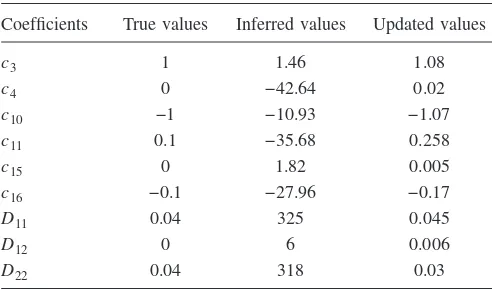
We now apply the algorithm described in the previous section to infer both the unknown state and the vector field of this system. An example of noise-corrupted measurements of the system共27兲is shown in Fig.1共a兲. Our technique allows recovery of the stochastic dynamics of the system 共27兲 as shown in Fig. 1共b兲 and to estimate model parameters. The results of the estimations are shown in TableI. It is evident that the optimization in the paths’ space can be performed
-2 0 2
-4 -2 0 2 4
y
x (a)
-1 0 1
-3 -2 -1 0 1 2 3
y
[image:5.609.361.508.67.313.2]x (b)
FIG. 1. 共a兲 Example of corrupted-by-noise measurements共27兲
efficiently in the presence of measurement noise. In practice, however, the conjugate gradient algorithm requires about 20 steps for convergence. The complexity of such an algorithm
共calculated as a number of matrix operations兲is much higher that the complexity of the calculations of the model param-eters using Eqs. 共10兲–共13兲. Accordingly, for the fast on-line applications of the algorithm one should avoid global opti-mization in the space of dynamical trajectories by, e.g., sup-pressing measurement noise.
The main focus in the remaining part of the research will be the development of the fast on-line tracking method for the time-varying parameters. For the sake of simplicity of our further arguments, we therefore assume that measure-ment noise can be neglected. In the next section, we will introduce a specific example of a model that can be applied for the interpretation of physiological time-series data using our Bayesian inferential framework.
IV. SYSTEM OF FITZHUGH-NAGUMO OSCILLATORS
In the context of physiological applications, we consider the following dynamical model 共see 关17兴 for details of the numerical analysis of this model兲:
x˙=f共x兩c兲−q+
冑
Dˆ共t兲, x=共x1, . . . ,xL兲, 共29兲q˙= −q+␥x, 共30兲 representing a set of independent FitzHugh-Nagumo sys-tems. The measurements are modeled by the following equa-tion:
y=Xˆ x. 共31兲 Note that the q coordinates are “hidden” or unobservable, while thex coordinates are accessible for measurement and are mixed by the measurement matrixXˆ.
The main assumptions of the model共29兲–共31兲are that the measurement noise can be neglected together with the noise in Eq.共30兲. Under these assumptions, sampling in the paths’ space can be avoided, thus paving the way to the fast on-line decoding of physiological information. Indeed, in this case Eq. 共30兲can be integrated,
q共t兲=␥
冕
0 tde−共t−兲x共兲+e−tq共0兲. 共32兲
Here q共0兲 is a set of initial coordinates that needs to be inferred along with the rest of the parameters. Therefore, the unobservable variables can be excluded from further consid-eration. According to the trapezoidal rule, the discrete ver-sion of Eq.共32兲is
q共tk兲=␥h
兺
r=0 ke−共tk−tr兲x共t r兲−
h␥
2 „x共tk兲+e −tk
x共t0兲…
+e−tkq共0兲. 共33兲
The resulting model and its discretization have the follow-ing form:
xk+1=hf共xk
*兩c兲−␥h2
兺
r=0 ke−共tk−tr兲x共t r兲
+h 2␥
2 关x共tk兲+e −tk
x共t0兲兴
−he−tkq共0兲+⌬
k+O共h2兲, 共34兲 where⌬k=兰tk
tk+1dt
⬘
共t⬘
兲 andxk
*⬅xk+1+xk
2 .
The FHN oscillator is a special case of the dynamics in Eqs. 共29兲 and共30兲. It will be the subject of our numerical experiments,
v˙j= −vj共vj−␣j兲共vj− 1兲−qj+j+djj,
q˙j= −qj+␥jvj,
具j共t兲i共t
⬘
兲典=␦ijdi␦共t−t⬘
兲, j= 1:L. 共35兲 The system described in Eq. 共35兲 represents the simplified dynamic of L noninteracting neurons关21兴, each of them la-beled with j;vjrepresents the membrane potential while qj are slow recovery variables.In practice, signals that are collected from biological sys-tems are mixed with a measurement matrix; to tackle this problem, we assume that the measurement variable is yi, which is a linear transformation ofvj,
yi=Xijvj. 共36兲 Here the mixing matrix Xis anunknown quantity, therefore yicontains all the accessible information. In Fig.2, there is an example of yias in Eq.共36兲.
To write explicitly the system to be inferred, expressions ofqifrom Eq.共33兲and ofviin Eq.共35兲are plugged into Eq.
共36兲. Within our inferential framework, this trajectory repre-sents the output of the following model:
y˙i=Aijyj+Bijlyjyl+Cijlmyjylym+˜i
−h
兺
r=0 ke−共tk−tr兲⌫
ilyl共tr兲−
兺
r=0 ke−tk˜z
i+Dijj+共t兲,
[image:6.609.49.295.95.240.2]共37兲 where˜zi are the components of the boundary conditionq共t
TABLE I. Convergence of some coefficients of the system共28兲. We have used one block of data with 40 000 points.
Coefficients True values Inferred values Updated values
c3 1 1.46 1.08
c4 0 −42.64 0.02
c10 −1 −10.93 −1.07
c11 0.1 −35.68 0.258
c15 0 1.82 0.005
c16 −0.1 −27.96 −0.17
D11 0.04 325 0.045
D12 0 6 0.006
= 0兲, and use of the following definitions was made: Aij=Xim␣m共X−1兲mj,
Bijl=Xim共1 +␣m兲共X−1兲mj共X−1兲ml,
Cjklm=Xji共X−1兲ik共X−1兲il共X−1兲im,
⌫il=Xij␥j共X−1兲jl. 共38兲 In Eqs.共38兲, a sum over repeated indices is implied and all the indices range from 1 toL. Also, the diffusion matrixDij is expressed in terms of djas
Dji=Xjidi. 共39兲 Finally, Eqs. 共38兲 contain the crucial model parameters ˜j that are the focus of our inference. They are related to the original model parametersjby
˜j=Xjii. 共40兲 We treatyj共t兲in Eqs.共38兲as measured variables. As a result of the inference procedure, we will recover the matrix ele-ments ofA,B,C,⌫,D,˜.
The parameters of the modified and original dynamical models can be learned effectively using stationary blocks of the time-series data, as will be shown using numerical ex-amples in paper II关17兴. Once the constant parameters of the model have been learned, the algorithm will allow for very fast on-line tracking of the time-varying control parameters. Details of the convergence of the model parameters and of the time resolution of the parameter tracking will be
pro-vided in paper II, using as an example synthetic time-series data generated by the model共29兲–共31兲.
V. CONCLUSION
Our Bayesian framework for the time-resolved inference of a nonstationary stochastic dynamical system allows for learning the parameters of the dynamical and measurement models from noise-corrupted time-series data with subse-quent fast tracking of time-varying control parameters. Con-vergence of the method in the parameter space, and global optimization in the space of dynamical trajectories, are dis-cussed. It is shown that to achieve the best time resolution, one has to embed the time tracking of nonstationary dynam-ics into an inferential learning framework that allows for preliminary inference of the model parameters in the station-ary regime. Furthermore, one has to reduce the measurement noise to a low level to avoid global optimization in the tra-jectory space, which is necessarily time-consuming. In doing so, one can improve the time resolution of the method by several orders of magnitude. To apply this technique to the real time decoding of information from nonstationary physi-ological time-series data, we introduce a specific model of FHN oscillators mixed by an unknown measurement matrix. Next we show how this model can be reduced to allow for the fast on-line tracking of nonstationary parameters in a Bayesian inferential framework. A numerical investigation of this system is presented and discussed in paper II 关17兴.
Note that for simplicity of the analysis, we have excluded dynamical noise from the equation for the recovery variable in Eq.共30兲 共cf., e.g.,关23兴兲. It is possible, however, to extend the proposed method to encompass the case of a stochastic linear differential equation for the hidden dynamical variable by adding a stochastic integral to the right-hand side of the reduced model 共34兲. The corresponding extension of the method will be discussed in more detail elsewhere.
Finally, we emphasize the broad interdisciplinary applica-tions of the method and we comment that it can readily be extended to take into account the effects of multiplicative and colored noise and of binary variables in the model.
ACKNOWLEDGMENTS
We are grateful to the Engineering and Physical Sciences Research Council共UK兲and NASA for financial support, and to A. Stefanovska for valuable discussions.
关1兴H. Konno and K. Hayashi, Ann. Nucl. Energy 23, 35共1996兲.
关2兴J. Christensen-Dalsgaard, Rev. Mod. Phys. 74, 1073共2002兲.
关3兴V. N. Smelyanskiy, D. G. Luchinsky, A. Stefanovska, and P. V. E. McClintock, Phys. Rev. Lett. 94, 098101共2005兲.
关4兴E. Izhikevich, Dynamical Systems in Neuroscience: The Ge-ometry of Excitability and Bursting 共MIT Press, Cambridge, MA, 2006兲.
关5兴S. Siegert, R. Friedrich, and J. Peinke, Phys. Lett. A 243, 275
共1998兲.
关6兴P. E. McSharry and L. A. Smith, Phys. Rev. Lett. 83, 4285
共1999兲.
关7兴R. Friedrichet al., Phys. Lett. A 271, 217共2000兲.
关8兴J. P. M. Heald and J. Stark, Phys. Rev. Lett. 84, 2366共2000兲.
关9兴R. Meyer and N. Christensen, Phys. Rev. E 62, 3535共2000兲.
关10兴R. Meyer and N. Christensen, Phys. Rev. E 65, 016206
共2001兲.
关11兴J.-M. Fullana and M. Rossi, Phys. Rev. E 65, 031107共2002兲.
关12兴M. Siefert, A. Kittel, R. Friedrich, and J. Peinke, Europhys. 0
1 2 3 4
0 4 8
t (ms)
V
[image:7.609.56.293.68.155.2]1
FIG. 2. 共Color online兲 Example of a typical component y共t兲
from Eq.共36兲with mixing matrix共1221兲. Values of the parameters are
␣1=␣2= 0.2, 1=2= 0.112, = 0.005 105 1, ␥1=␥2= 0.0051, d1
= 0.001, andd2= 0.002. Coefficients1and2change ranging from
Lett. 61, 466共2003兲.
关13兴F. Watanabe, H. Konno, and S. Kanemoto, Ann. Nucl. Energy
31, 375共2004兲.
关14兴W. Enders,Applied Econometric Time Series, 2nd ed.共Wiley, Hoboken, NJ, 2004兲.
关15兴V. N. Smelyanskiy, D. G. Luchinsky, D. A. Timucin, and A. Bandrivskyy, Phys. Rev. E 72, 026202共2005兲.
关16兴V. N. Smelyanskiy, D. G. Luchinsky, A. Stefanovska, and P. V. E. McClintock, Phys. Rev. Lett. 94, 098101共2005兲.
关17兴A. Duggentoet al., following paper, Phys. Rev. E 77, 061106
共2008兲.
关18兴V. V. Osipov, D. G. Luchinsky, V. N. Smelyanskiy, and D. A. Timucin, Proceedings of the AIAA/ASME/SAE/ASEE Joint Propulsion Conference and Exhibit, AIAA Conference Pro-ceedings共AIAA, Cincinnati, OH, 2007兲, p. 5823.
关19兴D. G. Luchinsky et al., Proceedings of the AIAA Infotech@Aerospace 2007 Conference and Exhibit, AIAA Con-ference Proceedings 共AIAA, Robnert Park, CA, 2007兲, p. 2829.
关20兴R. FitzHugh, Biophys. J. 1, 445共1961兲.
关21兴J. Nagumo, S. Animoto, and S. Yoshizawa, Proc. IRE 50, 2061
共1962兲.
关22兴A. T. Winfree, The Geometry of Biological Time 共 Springer-Verlag, New York, 1980兲.
关23兴E. V. Pankratova, A. V. Polovinkin, and B. Spagnolo, Phys. Lett. A 344, 45共2005兲.
关24兴J. Keener and J. Sneyd, Mathematical Physiology共 Springer-Verlag, New York, 1998兲.
关25兴E. N. Best, Biophys. J. 27, 87共1979兲.
关26兴J. Rogers and A. McCulloch, IEEE Trans. Biomed. Eng. 41, 743共1994兲.
关27兴R. R. Aliev and A. V. Panfilov, J. Theor. Biol. 181, 33共1996兲.
关28兴P. Chen, SIAM J. Math. Anal. 23, 81共1992兲.
关29兴O. Berenfeld and S. Abboud, Med. Eng. Phys. 18, 615共1996兲.
关30兴D. G. Luchinsky, V. N. Smelyanskiy, and J. Smith, in Un-solved Problems of Noise and Fluctuations, AIP Conf. Proc. No. 800, edited by L. Reggiani et al. 共AIP, Melville, NY, 2005兲, pp. 539–545.
关31兴R. Graham, Z. Phys. B 26, 281共1977兲.
关32兴A. Apte, M. Hairer, A. M. Stuart, and J. Voss, Physica D 230, 50共2007兲.
关33兴C. Calder, M. Lavine, P. Müller, and J. S. Clark, Ecology 84, 1395共2003兲.
关34兴V. N. Smelyanskiy, D. G. Luchinsky, and M. Millonas, e-print arXiv:physics/0601004v1.
关35兴D. G. Luchinsky, V. N. Smelyanskiy, M. Millonas, and P. V. E. McClintock,in Noise in Complex Systems and Stochastic Dy-namics III, Vol. 5845 ofProceedings of the Society of Photo-Optical Instrumentation Engineers (SPIE), edited by L. B. Kish, K. Lindenberg, and Z. Gingl 共SPIE, Bellingham, WA, 2005兲, pp. 173–181.