Spiking Neural Network Model of Sound
Localisation using the Interaural Intensity Difference
Julie A. Wall, Liam J. McDaid, Liam P. Maguire, and Thomas M. McGinnity
Abstract—In this paper, a spiking neural network (SNN) architecture to simulate the sound localisation ability of the mammalian auditory pathways using the interaural intensity difference (IID) cue is presented. The lateral superior olive (LSO) was the inspiration for the architecture which required the integration of an auditory periphery (cochlea) model and a model of the medial nucleus of the trapezoid body (MNTB). The SNN uses leaky integrate and fire excitatory and inhibitory spiking neurons, facilitating synapses and receptive fields. Experimentally derived Head Related Transfer Function (HRTF) acoustical data from adult domestic cats were employed to train and validate the localisation ability of the architecture; training used the super-vised learning algorithm called the Remote Supervision Method (ReSuMe) to determine the azimuthal angles. The experimental results demonstrate that the architecture performs best when it is localising high frequency sound data in agreement with the biology, and also shows a high degree of robustness when the HRTF acoustical data is corrupted by noise.
Index Terms—Spiking neural networks, sound localisation, lateral superior olive, interaural intensity difference
I. INTRODUCTION
O
F all the organs in the body, there are few that can com-pare to the ear with regards to the degree of functionality it contains within such a small and compressed space. Sound localisation is one such function that the ears and auditory pathways perform together and can be defined as the ability to determine the point of origin of a sound source. It is a powerful aspect of mammalian perception, allowing an awareness of the environment and permitting mammals to locate prey, potential mates and predators [1]. The neural components of sound localisation are complicated, as the location of a stimulus can only be determined by combining input from both ears [2].Mammalian sound localisation is determined with a com-bination of binaural cues; interaural time differences (ITDs), which are processed in the medial superior olive (MSO) for low frequency sound-signals (< 1.5 kHz in both humans and cats) and IIDs, which are processed in the LSO for high frequency sounds (> 2 kHz in humans and 5 kHz in cats) [3]. Both the LSO and MSO are located within an area of the auditory system called the superior olivary complex [3]. The combination of ITD and IID processing is better known as the “duplex theory of sound localization” and was first devised by Thompson and Rayleigh [4], [5]. ITD refers to the different points in time at which a sound from a single location arrives
Manuscript received December 23, 2010. The authors are with the Intelligent Systems Research Centre, School of Computing and Intelligent Systems, University of Ulster, Magee Campus. (phone: +44 (0)28 71375166; email: [email protected]). This research is supported under the Centre of Excellence in Intelligent Systems (CoEIS) project, funded by the Northern Ireland Integrated Development Fund and InvestNI.
at each individual ear [6]. From this time difference, the brain can calculate the angle of the sound source in relation to the head [7]. In this paper there is a focus on sound localisation by means of IID, defined as the difference in sound pressure levels (SPL) of the sound signal between each ear for a particular frequency, measured in decibels [3], [8].
In humans, the LSO appears as a folded sheet of excited-inhibited neurons with high characteristic frequencies in agree-ment with the duplex theory of sound localisation; it is signif-icantly smaller than the MSO [9]. The size of the LSO in different mammals is consistent with the range of usable fre-quencies, e.g. bats and porpoises which can process extremely high frequencies have large LSOs whereas humans are not as sensitive to such frequencies and as such have a smaller LSO [10], [11]. Cats are sensitive to both low and high frequencies with a frequency range of about 100 Hz to 50 kHz, and have an LSO which is equally prominent to its MSO [11]. The LSO favours high frequencies as the head casts a clearer shadow in the sound-scape producing differing SPLs at each ear for a particular sound source frequency [3], [12], [13], [14]. It should be noted that there have been some observations as to the functionality of the LSO in the presence of low frequency sound. It is thought that there are several different functions, e.g. the response of the LSO to low frequency sounds interacts with the response of the MSO at the inferior colliculus (IC) producing neurons with more distinct ITDs than if the LSO and MSO were working independently [15]. The LSO has a tonotopical organisation, high frequencies are represented in the middle of the LSO and continually lower frequencies to the sides [2]. It is excited by innervation from small spherical bushy cells of the ipsilateral anteroventral cochlear nucleus (AVCN) and inhibited by innervation from the contralateral MNTB. The MNTB receives input from globular bushy cells of the contralateral AVCN [2], [12].
For high frequency sound waves that have a similar or smaller wavelength than the diameter of the human head, a shadowing effect occurs on a sound wave approaching the contralateral ear [16]. This shadowing of the sound wave gives a difference of intensity between the two sound signals for each ear, i.e. the head acts as a low-pass filter causing IIDs of up to 20 dB SPL. Processing in the LSO involves taking as input the two sound signals in the form of a neural stimulus from each ear. The ipsilateral stimulus will take an excitatory form and the contralateral will be inhibitory having passed through the inhibitory MNTB. The interaction between the two stimuli works as a neural form of subtraction producing an output relating to the IID [3].
applications, from virtual reality to hearing aids. However, the power and speed of mammalian sound localisation can only enhance these applications. The ability to model the ways in which mammals localise a sound source can: allow for the development of better virtual realities; increase the intelligent behaviour of robotics; improve teleconferencing; provide surveillance systems with omni-directional sensitivity; improve the building of cinemas, opera houses and theatres by being aware of where to put sound-reflective surfaces; and enhance hearing aids by improving the localisation of individual sounds. These enhancements which are enabled by the ability to understand and model mammalian sound localisation provide the rationale for the research outlined in this paper.
The aim of this research involves the development of a model, using spiking neurons, which will process and extract the binaural cue of IID with a topology inspired by the mammalian auditory pathways. To that end, this research proposes to create a SNN model which emulates the way in which mammals localise sound. The reasoning for the use of SNNs is to maintain biological realism, i.e. spiking neurons are the most biologically inspired type of computational neuron model. Biological neurons process and circulate information by electrochemical signalling using spikes or action potentials, and spiking neurons can model this behaviour. Thus, topologies of spiking neurons can closely model a neural circuit. Our overall aim is to perform the task of sound localisation in real time in a biologically-inspired way using real biological data as input. To achieve this, the architecture presented benefits from both engineering principles in the form of machine learning and simple LIF spiking neurons; and biological inspiration based on the topology of the mammalian auditory system and its functional components.
The research presented in this paper builds on earlier work [17], [18] and involves the development of an SNN model which aims to mimic the architecture of the human auditory pathways, specifically the LSO, for the purpose of sound localisation. The SNN is trained with ReSuMe [19] to localise experimentally derived acoustical HRTF data to every 10°. The model employs an auditory periphery (cochlea) model which takes as input HRTF data for each ear and produces spike trains relating to the sound frequency and SPL of that input. All neurons in the architecture are implemented using a leaky integrate and fire (LIF) model. The architecture consists of two separate SNNs which reflect the bilateral symmetry of the nervous system, i.e. there is one model for each ear; one processes data corresponding to angles in the range of -60° to 0°; the other corresponds to angles in the range of 10° to 60°.
In this approach, the LSO neuron takes as input an excita-tory and inhibiexcita-tory input stimulus. The output, which can be considered a neural form of the IID, is routed through a layer of receptive fields (RF). The function of the RFs and their corresponding neurons is to respond to unique spike frequency ranges and to encode the output responses of the LSO into linear spike trains for ReSuMe to classify to angles of location; a linear spike train means that the spike train is generated using a constant interspike interval (ISI).
The paper is organised as follows. Section II provides a review of the current state of the art in sound localisation modelling while Section III will describe each layer of the SNN model of interaural intensity based sound localisation. Section IV will present the results achieved from both training and testing; and Section V draws the conclusions.
II. REVIEW
There are three distinct approaches to sound localisation modelling, namely statistical theory [20][21], signal processing with cross-correlation [22][23], and artificial neural networks (ANN). ANNs are mathematical or computational models which aim to imitate the framework and functionality of a biological neural network; the ideas for these types of networks came from physiological studies of the nervous systems of living beings. ANNs of the first generation consist of the simplistic McCulloch-Pitts threshold neuron models [24], while neurons of the second generation use a continuous activation function [25]. The most biologically inspired ANNs are those of the third generation, called SNNs, as individual spikes are used as input which allow for spatio-temporal information to be included in the computation [25]. Neural network-based research on auditory modelling takes a more biologically inspired approach in comparison to the statistical and signal processing approaches. Therefore, the following review will focus on the ANN and SNN techniques other researchers have used to develop sound source localisation models.
Palmieri et al. [26] used an ANN to imitate the sound localisation behaviour of the owl. Inputs to the system in-volve both binaural time and intensity cues to determine the azimuth and elevation of a sound source. The three-layered neural network was trained with the multiple extended Kalman algorithm. The error was determined by finding the difference between the estimated azimuthal position produced as output from the ANN against the actual position which was measured with an ideal optical sensor. Using simulated input data the average error produced was 1.86° and 0.81° for the elevation and azimuth respectively. Alim and Farag [27] used an ANN to localise sound using HRTFs generated from five human subjects. The IID was determined by calculating the SPL for every sound frequency at each ear, and the ITD was calculated by correlating the right and left ear HRTF data. The four-layered neural network was trained using back-propagation, and while results show an error of 25%, a comparison with localisation tests carried out on human subjects showed that both sets of results were very similar.
system was tested on pure tone sound signals between 120 Hz and 1.2 kHz, recorded in an anechoic chamber using the Darmstadt robotic head for angles in the range of ±105° in steps of 30°, giving a localisation efficiency of 59%. When tested for lateralisation, i.e. an estimation of the sound source position in the horizontal plane, an accuracy of almost 90% efficiency was achieved. Poulsen & Moore also demonstrated how SNNs could be combined with an EA to facilitate sound localisation [29]. They simulated a 2-dimensional environment wherein multiple agents possess an SNN which controls their movements based on binaural acoustical inputs. An EA was employed to evolve the connectivity and weights between neurons. A spike response model was selected for each neuron in the network and based on the position of the ears relative to the sound source the ITD and IID was determined. The EA updated an agents’ fitness score if they moved closer (increase) or further away (decrease) from the source. After training, most agents were able to localise single sound sources, however this ability decreased when multiple sound sources were tested.
Research by Liu et al. on the development of SNNs for sound localisation outlined an auditory processing system utilising both ITD and IID cues [30]. Input sound passes through a Gammatone filterbank and is then encoded into phase-locked spikes using a model of the halfwave rectified receptor potential of inner hair cells. ITD processing uses a series of delays and a LIF neuron model; the ITD is calculated for all frequency channels to form a full map of ITD processing. IID processing does not use a neuron model, rather a logarithmic ratio computes the intensity difference. Both ITD and IID spike outputs are routed through a model of the IC and conditional probability is used to modify the weights on each input. The model was tested using a robotic head on broadband sounds, both noise and speech, in the range of [±90°in steps of 30°] and achieved overall localisation accuracies of 80%. The model was also tested on multiple sound sources using two speakers with very encouraging results also.
In contrast to the purely computational or signal processing techniques, the ANN and SNN approaches are more biolog-ically inspired and when trained with real experimental data increase the biological credibility. The work presented in this paper differs from those above in that it uses experimentally derived HRTF data generated from adult domestic cats as input; performs sound localisation with a fine resolution of angles, i.e. can localise to every 10°; outlines results showing successful sound localisation across a wide range of high frequency sounds; and uses a biologically inspired learning algorithm to classify the outputs of the LSO model into distinct azimuthal angles. Also, only the IID auditory cue is used in this research as the aim is to model the functionality of the LSO and thus localise high frequency sounds in a biologically-inspired way. The training and testing accuracies presented are on a par with the other SNN-based research on biologically inspired sound localisation outlined in this review section.
[image:3.612.330.546.50.161.2]III. NETWORKTOPOLOGY
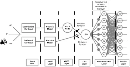
Fig. 1 outlines the proposed fully-connected feed-forward SNN architecture for sound localisation which consists of two
(a)SNN for angles originating from the range -60° to 0° (left network)
[image:3.612.330.546.199.305.2](b)SNN for angles originating from the range 10° to 60° (right network)
Figure 1:SNN architecture
separate SNN models reflecting the bilateral symmetry of the nervous system; one deals with data corresponding to the sound originating to the left of the head, i.e. angles in the range of -60° to 0° while the other deals with data corresponding to the sound originating to the right of the head, i.e. angles in the range of 10° to 60°. The reason for separating the azimuthal angles across two networks will become clear in Section B. MNTB and LSO Layer. For the remainder of this paper, the functionality of the left network will be described as both networks process data identically. However, results will be given for both networks in SectionIV.
Figure 2:Plan of the auditory periphery model, from [31], [32]
to the LSO neuron and the contralateral outputs of the cochlea are routed directly to the MNTB neuron. The network is now described in more detail.
A. Input Layer
The input layer consists of two auditory periphery (cochlea) models [31], [32], see Figure 2, based on empirical observa-tions in the cat. As such, this model is appropriate for the HRTF input data [33] used in this work as this data was taken from an anesthetised cat. There is one cochlea model for each ear, which encodes the input data into spike trains. HRTF data describes the acoustical gain (dB) in response to a sound before it reaches the cochlea after the diffraction and reflection properties of the head, pinna and torso have affected it. Data is available for thirty-six different azimuthal angles (-180° to 170° in bins of 10°) at 148 distinct sound frequencies (600 Hz to 30 kHz in steps of 200 Hz) for both the left and right ears. Thirteen angles are used for classification, corresponding to the angles±60° in steps of 10°. The angles within the range of ±60° were chosen as they constitute a continuous range of angles that can be linearly distinguished. However, this issue with linearity is not overly important as there is a set of HRTF data between ±60° for each individual ear. The data which is used for classification is the combination of the data from each ear, i.e. the output of the LSO layer. The 3-D mesh surface plot shown in Fig. 3 demonstrates the highly complex and non-linear nature of this data for a classification-type problem.
[image:4.612.323.550.51.162.2]Each cochlea takes the frequency and intensity of a sound source at a particular azimuthal angle as input and produces a spike train based on that input generated through an inhomo-geneous Poisson encoding process [34]. For the purposes of training the SNN to recognise and classify this data, multiple spike trains were generated for training and testing, see Figure
Figure 3: 3-D mesh surface plot of the right ear HRTF acoustical input data for the angles±60° across the range of sound frequencies from 600 Hz to 30 kHz in steps of 200 Hz.
Figure 4: 100 different neural outputs from the cochlea model for the -50° angle of the left input 15000 Hz sound frequency
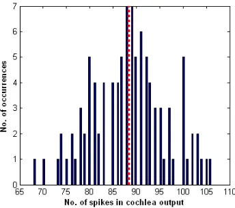
[image:4.612.333.548.223.446.2]Figure 5: Histogram plotting the range of output frequencies from the cochlea model for the -50° angle of the left input 15 kHz sound frequency. The red dotted line indicates the average output frequency. Those frequencies at the edge of the histogram, i.e. < 70 Hz are considered to be outliers and do not facilitate exact classification.
B. MNTB and LSO Layer
The MNTB layer, see Fig. 1, consists of an inhibitory LIF neuron which represents the neurons of the tonotopically organised by frequency MNTB. The model consists of one LIF neuron as it relates to a narrow frequency band of sound. This work considers the SNN to be akin to the subset of biological neurons assigned to dealing with a narrow frequency band of sound; multiple networks are required to process multiple sound frequencies. For computational efficiency, the same SNN structure with no change to parameters is reused to train and test multiple sound frequencies. The MNTB neuron takes the contralateral stimulus as input and converts it to an inhibitory stimulus with the same pattern and frequency of spikes. This output is then routed to the LSO layer. All LIF neurons in the network are modelled by [35]:
τmem
dv
dt =−v+RinIsyn(t) (1) where τmem refers to the membrane time constant of the
neuron,v is the membrane potential andRinis the membrane
resistance, driven by a synaptic currentIsyn(t).
It is now known that synapses of the neocortex are dynamic; neuron responses are not as simple as multiplication of a post-synaptic input by a post-synaptic weight, rather it is a reaction to short term input [36], [37]. There are two known types of dynamic synapses, facilitating synapses which can be found between pyramidal neurons and inhibitory interneurons, and depressing synapses which can also be seen between pyramidal neurons [38], [39]. Facilitating synapses gradually use their synaptic resources and produce a sustained response. Depress-ing synapses consume all of their resources in the first few spikes and become unresponsive thereafter.
The LSO layer, see Fig. 1, consists of a LIF neuron with excitatory and inhibitory facilitating synapses which closely model the functionality of the biological LSO. The human LSO consists of approximately 4,500 - 5,000 neurons organised tonotopically by frequency. Therefore, this work considers the
LIF neuron to be akin to the subset of biological neurons assigned to dealing with a narrow frequency band of sound. The LSO neuron takes input from the excitatory facilitating synapse and the inhibitory facilitating synapse via the con-tralateral MNTB neuron. The difference in these spike train frequencies relates to the IID and is reflected in the LSO output response, which is used to classify the azimuthal angle of the input stimulus in latter layers of the network. To calculate the difference, the excitatory and inhibitory post synaptic potentials (PSP) are summed; essentially the inhibitory PSP generates the neural equivalent of subtraction. Facilitating synapses are used in this layer as they produce a smooth PSP enabling the subtraction process to be more adept at producing the difference between the excitatory and inhibitory input stimuli. The resultant PSP generated from this summation is the input to the LIF neuron and the associated output response is a measure of the difference between the two input frequencies. Both inhibitory and excitatory facilitating synapses in this layer use the following differential equations [38]:
dx dt =
z τrec
−USEx(tsp) (2)
dy dt =−
y τin
+USEx(tsp) (3)
dz dt =
y τin
− z τrec
(4)
These equations depict the inactive(x), active(y)and recov-ered(z)states of the synapse where τrec is the recovery time
period,USE is a constant value which denotes the maximum
amount of neurotransmitter which can be released after each presynaptic spike arrives, tsp is the presynaptic spike arrival
time and τin is the inactivation period usually of a few
milliseconds. The postsynaptic current can then be determined using:
Isyn(t) =ASEy(t) (5)
where the current is calculated as being proportional to the fraction of resources in the active state(y);ASE is a constant
value which represents the absolute synaptic strength (weight) [38]. The equations in (2-5) model a depressing synapse. Facilitating synapses need an additional equation where USE
can increase with every input spike; the changeable value of USE is referred to as U1:
dU1 dt =−
U1 τf acil
+USE(1−U1)δ(t−tsp) (6)
where τf acil is the facilitation time constant and the initial
value ofU1 is the value ofUSE at the time of the first spike
[38]. Parameters chosen for the facilitating synapses can be found in [38].
Figure 6: Response of both (A) left and (B) right LSOs based on the interplay of the ipsilateral excitatory and contralateral inhibitory input [3].
(a)5 kHz sound
(b)15 kHz sound
Figure 7:LSO neuron output versus angle for the sound frequencies 5 kHz (a) and 15 kHz (b). It is possible to see where the clusters of training samples overlap between the angles, resulting in overlapping frequency selective RFs.
in the range of ±60°. The x-axis portrays the angles and the y-axis shows the output responses produced by the LSO neuron in response to the input data relating to each angle. With 0° as the centre point, the response to angles to the left and right are approximately mirror images of each other. The minimum output frequencies are produced at 0°, and as the sound source pans to the left/right of the head, i.e. to ±60°, the LSO output spike frequencies increase. The LSO output responses presented in Fig. 7 relate to the output of both SNN architectures combined, to show the response for all azimuthal
angles. Negative azimuths correspond to the origin of the sound signal being to the left of the head, whereas positive azimuths correspond to the sound originating from the right of the head. This is in accordance with the physiological data provided by [40], where it is also seen that the LSO discharge rates show a sigmoidal behaviour as the azimuthal angles increase in both the positive and negative ranges for the range of angles ±60°. It is this monotonic increase in spike train frequency that enables the classification of the input data to angles of location. This is the main reason for having separate networks assigned for angles to the left and right of the head respectively. One combined network would be unable to classify between -60° and 60°, -50° and 50°, and so on. The output frequencies were determined by counting the number of spikes in the spike train for a stimulus duration of 50 ms. The duration of a sound has no affect on the ability for azimuthal sound localisation, as long as there is a minimum duration of 3 ms [41], [42]. Therefore, the use of a 50 ms sound duration in this work is appropriate. Another point to note from Fig. 7 is that there is a spike train frequency overlap between neighbouring angles, i.e. individual samples produce the same response for multiple angles. The amount of overlap also varies with sound frequency; the LSO output responses for the 5 kHz sound overlap considerably more in comparison to the 15 kHz sound. As the rate of overlap between angles increases, the task of localisation becomes more difficult, i.e. classification of the 5 kHz sound is more complicated in comparison to classification of the 15 kHz sound. The proceeding layers (RF and output layer) of the network will aim to classify this overlapping data between angles using frequency selective RFs and a supervised learning algorithm. Lastly, from Fig. 7 it can be seen that the range of responses for each angle produced by the LSO neuron is wider for the 5 kHz sound than for the 15 kHz sound. This difference indicates that the RFs designed for each sound will vary greatly even with respect to the same angles, i.e. the RF designed for 0° at 5 kHz will be very different to the RF designed for 0° at 15 kHz. This difference in RF widths is consistent with Tollin and Yin [40] who report that the spatial RFs of LSO neurons for lower sound frequencies around 5 kHz are much wider than those for higher frequencies. Overall, Fig. 7 highlights the issues the supervised training algorithm will have with classifying the LSO outputs and also how the success of classification differs across varying sound frequencies.
C. Hidden Layer
[image:6.612.61.288.187.542.2]be processed at any one time by the SNN.
To overcome these difficulties, the hidden layer consists of a layer of RFs, see Fig. 1, which encode the LSO output spike train frequencies into linear spike trains for the supervisory learning algorithm to classify. RFs are thought to be located throughout the auditory pathways; each region consists of RFs representing an area of space which responds selectively to sound frequency [40]. It is also thought that auditory RFs are sensitive to ITD, IID and other monaural spectral cues [40], [43], [44]. Bohte et al. [45], [46] used RFs in their time-to-first spike algorithm where inspiration was taken from the local RFs of biological neurons. The RF is used to encode the delay of the first spike time at the input layer. Similarly, the RFs in this work take the form of a Gaussian function; a Gaussian function was chosen as it provided a smooth transition between the activation of neighbouring neurons:
yi=e−((xi−fo)/dm)
2
(7)
whereyiis the output spike train frequency of the RF,xiis the
input frequency which has been routed from the LSO layer,fo
is the operating frequency of the RF anddmdenotes the width
of the RF. A RF was created for every angle being processed by the network using the half maximum distance method from fuzzy logic systems and radial basis function networks [47]. Each RF was assigned an operating frequency and width based on the LSO output frequencies of the specific angle assigned to it. To determine the operating frequency and width of each RF the following steps were taken. For each angle, 100 spike trains were generated from the left and right cochleas and these trains were routed through the LSO layer. The frequency of each train was found by counting the number of spikes over the time-length of the spike train. Unlike linear spike trains, the ISI cannot be used to determine the frequency of a Poisson spike train. The average spike train frequency produced by the LSO neuron becomes the operating frequency of the RF. The width of the RFdmreflects the spread in the spike train frequencies
about fo.
Originally, each RF was assigned the same arbitrarily cho-sen width. In some cases this value was too narrow and some samples of data did not activate their own designed RFs. Similarly, in other cases this value was too large and neighbouring RFs overlapped too much causing difficulty with classification. Fine-tuning of the RFs led to the use of the above process to determine the widths and operating frequency for each individual RF. In any case, when training and testing the network, samples will predominantly pass through a particular RF with some overlap with neighbouring RFs; hindering the selectivity of the neurons to individual angles.
The function of the RFs and their respective neurons is to scale the LSO output response to fall into the arbitrarily chosen range of [0, 40 Hz]. If the LSO output spike train frequency equals the operating frequency, the maximum frequency is encoded to be routed to the output layer for classification. Similarly, if an input frequency does not lie within the scope of the RF, the minimum frequency of 0 Hz is encoded. This is illustrated by Fig. 8. An input frequency, xi, routed from
[image:7.612.361.517.51.136.2]the LSO activates both RFs, A and B. As the input equals
Figure 8:Behaviour of RFs in response to incoming stimulus
Figure 9: Outputs of left RF layer neurons for the 15 kHz sound frequency. The input to these neurons is routed from the LSO which is filtered by RFs.
the operating frequency, fo, of RF A, that RF produces a
maximum output frequency,yA. However, the same input,xi,
only activates the edge of RFB, thus producing a lower output frequency,yB. It is this behaviour which enables the
separabil-ity of the input data to differing angles of location. It should be noted that this re-scaling method of LSO responses is identical for all LSO spike train outputs; hence the relationship between spike train frequencies of the LSO output was preserved.
Fig. 9 shows the RFs created for the 15 kHz sound and subsequent LSO output for the angles -60° to 0°, see Fig. 7(b), and the corresponding output response of each encoding neuron. Each RF and encoding neuron is assigned an angle of location, i.e.Ais -60°,Bis -50°, etc. As the input data for each angle is processed by the network, it is clear to see how each RF and corresponding encoding neuron respond. For example, encoding neuronAresponds maximally when data for the -60° angle is routed through the network; produces a more muted response when data for the -50° angle is processed, as the two RFs,AandB, for -60° and -50° overlap; and there is no response when data from the other five angles are processed. When there is little or no overlap between neighbouring RFs, for exampleC,DandE, the encoding neurons produce a crisp output response.
[image:7.612.326.550.165.357.2]de-creases the complexity of assigning the angle data to individual neurons in the output layer.
D. Output Layer
The output layer consists of seven LIF neurons relating to the angles -60° to 0° in steps of 10°, see Fig. 1(a). The learning algorithm used in this research is ReSuMe [19]. The aim of training is to map the input data to the correct angle where the highest firing frequency determines the classification.
ReSuMe [19] learning is similar to Supervised Hebbian Learning (SHL) [48] in that a supervisory (target) signal (spike train) is used to supervise the network during training. However ReSuMe, unlike SHL learning, does not feed these target signals directly to the current learning output neuron. Instead it controls the update of the synaptic efficacies on the active connections leading to the learning output neuron. Hence, the name remote supervision. The goal of ReSuMe is to train an SNN to produce a desired output in response to a given input. The learning rule modifies the synaptic weights between the RF layer encoding neurons and the output neurons using a remote supervisory signal. This modification is done using [19]:
d
dtwki(t) = Sd(t)
ad+
Z ∞
0
Wd(sd)Sin(t−sd)dsd
+
Sout(t)
aout+
Z ∞
0
Wout(sout)Sin(t−sout)dsout
(8)
where dtdwki(t) is the rate of change of the weights over
time, Sd(t) is the remote supervisory signal, Sin(t) refers
to the input spike trains, Sout(t) is the actual output of the
output neurons, ad and aout are the amplitudes of the
non-Hebbian processes of weight modifications and Wd(sd) and
Wout(sout) are the learning windows themselves. ReSuMe can be considered a biologically plausible learning rule as it is based on Hebbian learning and evidence has been found for remote supervision in biological synapses [49]. The main advantage of using ReSuMe over the similar learning algorithm of SHL, is that ReSuMe can increase synaptic weights that have been reduced to zero if those synaptic weights are required at a later epoch [50].
[image:8.612.339.532.51.231.2]Each output neuron was trained to be associated with a particular angle. During each epoch of training, the network was fed the training data for each angle in sequential order from -60° to 0°. For instance, input data for both ears corresponding to an angle of -60° was routed through the network to all the output neurons. This data passes through the RF layer onto one or more of the corresponding encoding neurons, see Figure 1(a). The encoding neurons pass the stimulus to each neuron in the output layer. Several spike trains will pass through more than one RF but the appropriate RF should produce the highest output frequency. Consistent with ReSuMe, the connections from the neuron producing the highest frequency will undergo the maximum weight updates. In the present case, multiple
Figure 10:Stable weight distribution over fifteen epochs of training on the connections between the RF and output layer neurons, 15 kHz sound and angles -60° to 0°.
samples of differing spike train frequencies exist for each angle and ReSuMe will produce a set of final weights for correct classification.
The same supervisory target signal was used for training every output neuron. The target signal consisted of an in-dependently generated high frequency linearly encoded spike train; a high frequency spike train was used to maximise the number of weight updates. Using the same target signal ensures that training is equal for all output neurons, and allows the network structure to be reproducible for training other sounds without changing parameters to suit any angle or sound. Fig. 10 shows the weight values produced by training over fifteen epochs; these weights are located on the connections between the RF layer neurons and output neurons. The weights stabilise over the course of training with many of the weights on the connections falling below zero while others stabilise at a positive value, this distribution of weights is what enables the network to associate new input data to the correct angle of location. In the case of this system, the contribution of any inhibitory weights in the output layer is negligible. During training, the weights fall below zero to such a small amount that the connections are effectively switched off. Some researchers place a cap on weights during training to disallow them falling below zero and increasing above a certain value, however the authors of this work prefer not to place artificial limits on weights.
IV. RESULTS
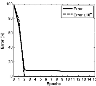
Figure 11:Overall training error for fifteen epochs of training across the angles -60° to 0° for the 15 kHz sound showing the accuracy for the desired angle alone and the accuracy for the desired angle ±10°.
testing data corresponds to newly generated and unseen 5 kHz data, and the neighbouring sound frequencies 4.8 kHz and 5.2 kHz respectively. These last two test vectors ensure that the network is tested with completely unseen sound frequencies.
The classification accuracy of the network is determined by the output neuron that is firing with the highest frequency. In this way, if the unseen data presented to the network during the testing phase produced the highest firing frequency at its intended output neuron, the SNN model is deemed to have made a correct classification. Results are now presented in two different ways. The first type of classification, termed here as absolute classification,is where the actual angle produced by the network is equal to the desired angle. The second type of classification takes into account the possibility of the network producing an angle at its output which is equal to the desired angle ±10°, i.e. if the desired angle is 30°, an output of 20° or 40° is also deemed acceptable. Fig. 11 plots the training accuracy for the 15 kHz sound source over fifteen epochs of training. After nine epochs, the absolute classification accuracy reaches 92.86%, however after only two epochs the desired angle classification±10° reaches 100%.
Initial experiments involved training with three different sound frequencies of 5 kHz, 15 kHz and 25 kHz. The weighted average generalisation testing results for angles in the range (±60° in steps of 10°) can be seen in Table I. The weighted average represents the classification accuracy of the SNN across all angles, i.e. the accuracies from both left and right networks are averaged together using the following weighted averageformula:
(7∗al) + (6∗ar)
13 (9)
whereal is the accuracy of the left network which has seven
angles, -60° to 0°, andaris the accuracy of the right network
which has six angles, 10° to 60°.
The network performed at its best when trained and tested with the 15 kHz sound, achieving absolute classification ac-curacies of approximately 80% and with ±10° resolution, the classification accuracy increases to approximately 99%. The results for the 5 kHz sound were lower, with absolute
Table I:Initial testing results for three sound frequencies, 5 kHz, 15 kHz and 25 kHz
Sound Generalisation Accuracy (%)
Accuracy±10° (%)
4.8 kHz 49.10 86.92
5 kHz 52.49 86.15
5.2 kHz 40.15 84.15
14.8 kHz 76.54 98.46
15 kHz 83.07 100
15.2 kHz 78.85 96.15
24.8 kHz 43.46 74.62
25 kHz 39.99 71.54
25.2 kHz 41.93 69.23
classification accuracies of 48% and for the ±10° resolution approximately 84%. The 25 kHz sound performed the worst with absolute classification accuracies of 43% and for the ±10° resolution approximately 72%. This result is consistent with Tollin and Yin [40] who reported that IIDs vary non-monotonically with azimuth at this very high sound frequency and thus are difficult to classify. Even though the absolute classification accuracies are low, the classification accuracies in the±10° column from Table I are considerably higher and therefore, it is reasonable to say that there is a degree of classification occurring, i.e. the angle of the incoming sound is being localised to the neighbouring angle in most cases, not a random and completely incorrect non-neighbouring angle.
Sound localisation differs from many classification tasks in that there is a relationship between the classes (angles). The difference between the experimental input data corresponding to neighbouring angles is small and in some cases identical for particular sound frequencies. This makes the task of dis-tinguishing between neighbouring angles difficult for the SNN model. Conversely, in most cases, non-neighbouring angles can be more easily distinguished by an SNN. This is arguably why many researchers present results using a coarser selection of angles, usually in steps of 30° [28], [30]. The results presented here show that when a margin of error of 10° is allowed, the classification results are significantly improved, as can be seen from Table I.
Each time the network was trained with a particular sound frequency, it was tested on that and two additional neighbour-ing sound frequencies over the range of angles ±60°, see Table I. It is interesting that not only is there a relationship between neighbouring angles in the input data, but there is also a relationship between neighbouring sounds, as the SNN can be used to process to a high classification accuracy multiple sounds. Using neighbouring sounds also gave the advantage of testing the network on completely unseen data.
[image:9.612.318.557.79.258.2]Figure 12: Classification results when tested by the entire range of sound frequencies,600Hz≤f≤30kHz
the total number of sound frequencies available and use the re-maining two-thirds for testing. This equates to thirty-one sound frequencies for training and sixty-two neighbouring sound frequencies for testing. This was an exhaustive but informative undertaking regarding the relationship of neighbouring sound frequencies and their classification accuracy. It was envisaged that the models would produce the best classification accuracies for high frequency sounds. The results of these experiments can be seen in Fig. 12, where the weighted average classification accuracy for both the left and right networks are reported along with the weighted average classification accuracy±10°.
As expected, the models achieve high classification accura-cies for high frequency sounds, ≥4 kHz, but do not localize well for sounds ≤4kHz. Low frequency sounds, ≤1.8kHz, are localized using the binaural cue of ITD and the MSO. Therefore, using the IID binaural cue for this band of sounds, it was expected that the localisation accuracies would be poor. For the intermediate range between high and low frequencies,
1.8kHz ≥ f ≤ 4.2kHz, neither the ITD nor IID binaural cues are proficient. This can be seen in biology, where the crossover between low and high frequency sounds cannot be localised to any great accuracy [51]. However, the overall classification results are quite high. There are two areas where the localisation ability of the IID model is lower than normal, around 10 kHz and above 25 kHz. These problems seemed to come from the experimental HRTF input data. The gain values across all of the input data are at their maximum around these sound frequencies. Initial experiments for these sound frequencies produced very low classification results. The HRTF data was scaled to counteract this problem and the results did improve but those problematic sound frequencies continued to achieve the lowest results across the entire range of sound frequencies. Furthermore, as previously stated, sounds ≥ 25
kHz are difficult to classify due to the variability of IIDs, providing further insight for the lower classification accuracies within this range.
A significant consideration when modelling mammalian sound localisation is the ability to localise a sound source in the midst of noise. Jacobsen [52] determined that when a pure tone signal is presented along with white noise, the ability to localise that pure tone is only compromised when the signal to noise ratio (SNR) falls below 20. The SNR defines how much of the original signal has been corrupted by noise. In
the present case, the signal relates to the HRTF input data and the noise is white Gaussian noise. SNR can be defined as:
SN R=Psignal
Pnoise
(10)
where P is the average power. Good and Gilkey [53] also performed thorough investigations on the affect of noise and found that a broadband click can be localised until the SNR falls into the negative range.
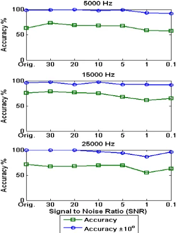
It was deemed necessary to determine whether the SNN models of sound localisation presented in this research would have similar performance abilities to those experiments dis-cussed above. To do this, white Gaussian noise was added to the HRTF data for the 5 kHz, 15 kHz and 25 kHz sounds and the models were retested to evaluate the classification accuracies. A range of SNRs were chosen for this task: 0.1, 1, 5, 10, 20 and 30. The MATLAB awgn function was used to incorporate the white Gaussian noise into the HRTF input data. Fig. 13 plots the classification accuracies when the SNN models are tested with noisy data. Each subplot shows the classification accuracy of the original non-noisy data and for the five different SNRs added to the original HRTF data. For each sound, the classification accuracies decrease almost monotonically with SNR. However, in some cases, higher SNR ratios report lower accuracies than for the same sound with a lower SNR. For example, the input data for the 15 kHz sound with an SNR of 0.1 produces higher classification accuracies than for the same input with an SNR of 1. This can be explained by the Poisson encoding scheme at the input layer and the random nature of adding noise to data itself. However, the three sounds tested showed a high degree of robustness to all the levels of noise, in agreement with the experiments described by [52], [53], i.e. the SNN maintained the ability to localise the input data to a high standard when it was contaminated with noise.
Figure 13: Classification accuracies when noise is added with five levels of SNR, from 0.1 to 30, where Orig. refers to the original classification accuracies of each sound with no added noise.
Experimental results show that the LSO networks only generalise well when the input data of the testing sound frequency is similar to the input data from the sound frequency used to train the SNN model. As the frequency of the sounds increase, the RF configurations have to be adapted to cater for the differing ranges of spike frequencies. This can be seen from Fig. 7, where the range of output frequencies from the LSO neurons for each angle differs between the two sound frequencies, 5 kHz and 15 kHz. The LSO neuron produces out-put frequencies across the angles ±60° which range between 250 Hz and 600 Hz. In contrast, when presented with the 15 kHz sound, a wider range of frequencies are produced by the LSO neuron, ranging from 50 Hz to 600 Hz. This indicates that differing sound frequencies far removed from each other require different RF parameters for the ability to localise the HRTF input data. Nevertheless, when the RF configurations are appropriate for the input data, testing accuracies for non-neighbouring sounds are quite good.
[image:11.612.360.512.53.185.2]Fig. 14 plots the testing accuracy of the LSO model for the 5 kHz sound frequency. It also shows the classification accuracies achieved when tested with lower and higher non-neighbouring sound frequencies. The lower frequencies of 3.8 kHz, 4 kHz and 4.2 kHz achieve a 0% classification accuracy, i.e. the RF configurations are so different between the 5 kHz sound and these lower sound frequencies that no data can be routed through the appropriate RF to the output layer. The higher frequencies of 5.8 kHz, 6 kHz and 6.2 kHz produce decreasing classification accuracies as the sound frequency increases. Yet, the classification accuracies±10° do not change with the increasing sound frequencies. In these cases, the RF parameters are adequate for these higher non-neighbouring
Figure 14:Generalisation across non-neighbouring sounds
Table II: Comparison of SNN and ANN sound localisation gener-alisation results for three sound frequencies, 5 kHz, 15 kHz and 25 kHz
SNN ANN
Sound Generalisation Accuracy (%)
Accuracy±10° (%)
Generalisation Accuracy (%)
4.8 kHz 66.02 96.15 78.08
5 kHz 63.07 98.46 94.95
5.2 kHz 70.76 99.23 89.12
14.8 kHz 72.17 95.38 92.34
15 kHz 75.76 96.15 86.93
15.2 kHz 73.07 96.92 87.02
24.8 kHz 69.23 100 94.55
25 kHz 71.02 100 91.51
25.2 kHz 60.38 95.38 77.39
sound frequencies.
Finally, the overall aim of this work was to perform the task of sound localisation in real time in a biologically-inspired way using real biological data as input. To achieve this, the architecture presented benefits from both engineering princi-ples in the form of machine learning and simple LIF spiking neurons; and biological inspiration based on the topology of the mammalian auditory system and its functional components. As the model is used as an engineering solution, to perform sound localisation, it was deemed necessary to compare it to a baseline classifier. In this case, we chose to compare the results of the SNN against a second generation artificial neural network (ANN), with the constraint that both the ANN design and the results should be comparable.
[image:11.612.310.567.260.451.2]and testing. However, the ANN which produced the optimum results as seen in Table II had three layers; thirteen input neurons, two hidden layers neurons activated with a hyper-bolic tangent sigmoid transfer function and one output neuron activated with a linear transfer function; and was trained with the Levenberg-Marquardt backpropagation algorithm.
As expected, the ANN classification results are more ac-curate than the SNN, as the ANN is widely considered to be a universal approximator. However, the ANN is a black box which provides no information on biological behaviour. Meanwhile, even though SNNs are still in their infancy, with the same input data set, the SNNs do achieve impressive results using more complex and biologically inspired neurons, architecture, and learning algorithm.
V. CONCLUSIONS
This paper presents a biologically inspired SNN-based archi-tecture of the mammalian auditory pathways. Experimentally derived HRTF data for each ear is used as input to the model and the IID binaural cue is extracted and used to localise that input to azimuthal angles. In comparison to the related work, this research provides novelty and advances significantly in this domain by using: topologies which are faithful to the architecture of the mammalian auditory pathways; a wide range of sound frequencies to test the localisation ability of the architecture; the utilisation of real experimental data rather than simulated data; and a fine resolution of angles. Additionally, to evaluate the capabilities of the SNN model, a biologically plausible supervised learning algorithm was used to train the architecture to localise the input data to a high degree of accuracy. Analysis of the processing abilities of the SNN with regards to robustness of localisation in the midst of noise and its generalisation capabilities are outlined. The experimental results derived from testing the full range of sound frequencies showed that this model behaves in a similar manner to the mammalian auditory pathways which process the binaural cue of IID, with regards to its ability to successfully localise high frequency sounds and issues with localising low frequency sounds. For these reasons, the authors believe the work presented in this paper is a significant step forward in biological sound localisation modelling.
Further work is planned which will involve implementation of the architecture on a mobile robot to perform sound locali-sation in an echoic and noisy environment. Extra functionality will be developed to enable the mobile robot to localise complex sounds and to discriminate between multiple sound sources. Additionally, this research will be extended to the modelling of regions higher up in the auditory pathways, i.e. the lateral lemniscus and IC.
VI. ACKNOWLEDGEMENT
Our thanks go to Dr. D. J. Tollin at the University of Colorado Med-ical School for providing us with the HRTF data and recommending which auditory periphery models to use. He was also invaluable for answering any queries we had over the course of this research.
REFERENCES
[1] D. McAlpine and B. Grothe, “Sound localization and delay lines - do mammals fit the model?,”Trends Neurosci, vol. 26, no. 7, pp. 347–350, 2003.
[2] T. C. T. Yin,Integrative Functions in the Mammalian Auditory Pathway, ch. Neural mechanisms of encoding binaural localization cues in the auditory brainstem, pp. 99–159. Springer-Verlag, 2002.
[3] D. J. Tollin, “The lateral superior olive: A functional role in sound source localization,”Neuroscientist, vol. 9, no. 2, pp. 127–143, 2003. [4] S. P. Thompson, “On the function of the two ears in the perception of
space,”Philos Mag, vol. 13, no. 83, pp. 406–416, 1882.
[5] L. Rayleigh, “On our perception of sound direction,” Philos. Mag, vol. 13, no. 74, pp. 214–232, 1907.
[6] M. S. Lewicki, “Sound localization 1,” 2006.
[7] B. Grothe, “New roles for synaptic inhibition in sound localization,”
Nature Rev Neurosci, vol. 4, no. 7, pp. 540–550, 2003.
[8] W. M. Hartmann, “How we localize sound,” Physics Today, vol. 52, no. 11, pp. 24–29, 1999.
[9] G. D. Pollak, R. M. Burger, T. J. Park, A. Klug, and E. E. Bauer, “Roles of inhibition for transforming binaural properties in the brainstem auditory system,”Hear Res, vol. 168, no. 1-2, pp. 60–78, 2002. [10] J. K. Moore, “Organization of the human superior olivary complex,”
Microsc Res Tech, vol. 51, no. 4, pp. 403–412, 2000.
[11] I. Bazwinsky, H. Hilbig, H. J. Bidmon, and R. Ruebsamen, “Charac-terization of the human superior olivary complex by calcium binding proteins and neurofilament H (SMI-32),”J Comp Neurol, vol. 456, no. 3, pp. 292–303, 2003.
[12] D. of Otorhinolaryngology, “Auditory 2: Central mechanisms,” 2002. University of Pennsylvania Health System.
[13] W. A. N. Dorland, D. M. Anderson, J. Keith, P. D. Novak, and M. A. Elliott,Dorland’s Illustrated Medical Dictionary. Saunders Philadelphia, 2003.
[14] R. Z. Shi and T. K. Horiuchi, “A VLSI model of the bat dorsal nucleus of the lateral lemniscus for azimuthal echolocation,” inProc. IEEE Int. Symp. Circuits Syst (ISCAS), pp. 4217–4220, 2005.
[15] D. J. Tollin and T. C. T. Yin, “Interaural phase and level difference sensitivity in low-frequency neurons in the lateral superior olive,” J Neurosci, vol. 25, no. 46, pp. 10648–10657, 2005.
[16] V. Willert, J. Eggert, J. Adamy, R. Stahl, and E. Korner, “A probabilistic model for binaural sound localization,”IEEE Trans. Syst. Man Cybern. B., vol. 36, no. 5, pp. 982–994, 2006.
[17] J. A. Wall, L. J. McDaid, L. P. Maguire, and T. M. McGinnity, “Spiking neuron models of the medial and lateral superior olive for sound localisation,” inIEEE Int. Joint Conf. Neural Networks (IJCNN) (IEEE World Congr. Computational Intelligence), pp. 2641–2647, 2008. [18] B. Glackin, J. A. Wall, T. M. McGinnity, L. P. Maguire, and L. J. McDaid,
“A spiking neural network model of the medial superior olive using spike timing dependent plasticity for sound localisation,”Front. Comput. Neurosci, vol. 4, pp. 1–16, 2010.
[19] F. Ponulak, “ReSuMe - New supervised learning method for spiking neural networks,” tech. rep., Institute of Control and Information Engi-neering, Poznan University of Technology., 2005.
[20] K. D. Martin, “Estimating azimuth and elevation from interaural dif-ferences,” in IEEE ASSP Workshop Applicat. Signal Process. Audio Acoust.z, pp. 96–99, 1995.
[21] W. Chau and R. O. Duda, “Combined monaural and binaural localization of sound sources,” in Proc. IEEE 29th Asilomar Conf. Signals Syst. Comput., vol. 2, pp. 1281–1285, 1995.
[22] J. M. Valin, F. Michaud, J. Rouat, and D. Letourneau, “Robust sound source localization using a microphone array on a mobile robot,” inProc. IEEE/RSJ Int. Conf. Intelligent Robots Syst. (IROS), vol. 2, pp. 1228– 1233, 2003.
[23] J. Murray, H. Erwin, and S. Wermter, “Robotic sound-source localization and tracking using interaural time difference and cross-correlation,” in
Proc. NeuroBotics Workshop, pp. 89–97, 2004.
[24] W. S. McCulloch and W. Pitts, “A logical calculus of the ideas immanent in nervous activity,” Bull. Math. Biophys., vol. 5, no. 4, pp. 115–133, 1943.
[27] O. A. Alim and H. Farag, “Modeling non-individualized binaural sound localization in the horizontal plane using artificial neural networks,” inProc. IEEE-INNS-ENNS Int. Joint Conf. Neural Networks (IJCNN), vol. 3, pp. 642–647, 2000.
[28] K. Voutsas and J. Adamy, “A biologically inspired spiking neural network for sound source lateralization,”IEEE Trans. Neural Netw., vol. 18, no. 6, pp. 1785–1799, 2007.
[29] T. M. Poulsen and R. K. Moore, “Sound localization through evolutionary learning applied to spiking neural networks,” inIEEE Symp. Foundations Computational Intell. (FOCI), pp. 350–356, 2007.
[30] J. Liu, D. Perez-Gonzalez, A. Rees, H. Erwin, and S. Wermter, “A biologically inspired spiking neural network model of the auditory midbrain for sound source localisation,”Neurocomputing, vol. 74, no. 1-3, pp. 129–139, 2010.
[31] M. S. A. Zilany and I. C. Bruce, “Modeling auditory-nerve responses for high sound pressure levels in the normal and impaired auditory periphery,”J. Acoust. Soc. Am., vol. 120, no. 3, pp. 1446–1466, 2006. [32] M. S. A. Zilany and I. C. Bruce, “Representation of the vowel /ε/
in normal and impaired auditory nerve fibers: Model predictions of responses in cats,”J. Acoust. Soc. Am., vol. 122, no. 1, pp. 402–417, 2007.
[33] D. J. Tollin, “The development of the acoustical cues to sound localiza-tion in cats,”Assoc. Res. Otol., vol. 27, p. 161, 2004.
[34] J. Virtamo, “Poisson process,” 2005.
[35] W. Gerstner and W. M. Kistler,Spiking Neuron Models: Single Neurons, Populations, Plasticity. Cambridge University Press, 2002.
[36] M. J. Denham, “The dynamics of learning and memory: Lessons from neuroscience,”S. Wermter, J. Austin, and D. Willshaw, editors, Emergent neural computational architectures based on neuroscience, vol. 2036, pp. 333–347, 2001.
[37] A. P. Shon and R. P. N. Rao, “Temporal sequence learning with dynamic synapses,” tech. rep., University of Washington, 2002.
[38] M. Tsodyks, K. Pawelzik, and H. Markram, “Neural networks with dynamic synapses,”Neural Computation, vol. 10, no. 4, pp. 821–835, 1998.
[39] L. F. Abbott, J. A. Varela, K. Sen, and S. B. Nelson, “Synaptic depression and cortical gain control,”Science, vol. 275, no. 5297, pp. 221–224, 1997. [40] D. J. Tollin and T. C. T. Yin, “The coding of spatial location by single units in the lateral superior olive of the cat. I. Spatial receptive fields in azimuth,”J. Neuroscience, vol. 22, no. 4, pp. 1454–1467, 2002. [41] P. Hofman and A. Van Opstal, “Spectro-temporal factors in
two-dimensional human sound localization,”J. Acoust. Soc. Am., vol. 103, p. 2634, 1998.
[42] J. Vliegen and A. Van Opstal, “The influence of duration and level on human sound localization,”J. Acoust. Soc. Am., vol. 115, p. 1705, 2004. [43] J. C. Zella, J. F. Brugge, and J. W. H. Schnupp, “Passive eye displacement alters auditory spatial receptive fields of cat superior colliculus neurons,”
Nature Neuroscience, vol. 4, no. 4, pp. 1167–1168, 2001.
[44] J. L. Pena and M. Konishi, “Auditory spatial receptive fields created by multiplication,”Science, vol. 292, no. 5515, pp. 249–252, 2001. [45] S. M. Bohte, H. La Poutré, and J. N. Kok, “Unsupervised clustering
with spiking neurons by sparse temporal coding and multilayer RBF networks,”IEEE Trans. Neural Netw., vol. 13, no. 2, pp. 426–435, 2002. [46] S. M. Bohte, J. N. Kok, and H. La Poutre, “Error-backpropagation in temporally encoded networks of spiking neurons,”Neurocomputing, vol. 48, pp. 17–38, 2003.
[47] G. Bugmann, “Normalized Gaussian radial basis function networks,”
Neurocomputing, vol. 20, no. 1, pp. 97–110, 1998.
[48] D. Hebb, The organization of behavior: a neuropsychological theory. Wiley, 1949.
[49] F. Ponulak and A. Kasinski, “Supervised learning in spiking neural networks with resume: Sequence learning, classification and spike-shifting,”Neural Computation, vol. 22, no. 2, pp. 467–510, 2010. [50] A. Kasinski and F. Ponulak, “Comparison of supervised learning methods
for spike time coding in spiking neural networks,”Int. J. Appl. Math. Comput. Sci., vol. 16, no. 1, pp. 101–113, 2006.
[51] Z. Zhou, “Sound localization and virtual auditory space,” tech. rep., University of Toronto, 2002.
[52] T. Jacobsen, “Localization in noise,” tech. rep., Technical University of Denmark Acoustics Laboratory, 1976.
![Figure 2: Plan of the auditory periphery model, from [31], [32]](https://thumb-us.123doks.com/thumbv2/123dok_us/445066.1043975/4.612.323.550.51.162/figure-plan-auditory-periphery-model.webp)
![Figure 6: Response of both (A) left and (B) right LSOs basedon the interplay of the ipsilateral excitatory and contralateralinhibitory input [3].](https://thumb-us.123doks.com/thumbv2/123dok_us/445066.1043975/6.612.61.288.187.542/figure-response-right-basedon-interplay-ipsilateral-excitatory-contralateralinhibitory.webp)