A CROSS-SHORE BEACH PROFILE EVOLUTION MODEL
MANTRIPATHI PRABATH RAVINDRA JAYARATNE
School of Architecture, Computing and Engineering University of East London, Docklands Campus
4-6 University Way, London E16 2RD, UK Tel: +44-208-223-2536; Fax: +44-208-223-2963
MD REZAUR RAHMAN
Department of Civil and Environmental Engineering University of South Florida
4202 E. Fowler Avenue Tampa, FL 33620-5350, USA
TOMOYA SHIBAYAMA
Department of Civil and Environmental Engineering, Faculty of Science and Engineering,
Waseda University,
3-4-1 Okubo, Shinjuku-ku, Tokyo 169-8555, Japan Tel/Fax: +81-3-5286-8296
Abstract
Developing an accurate and reliable time-averaged beach profile evolution model under normal and storm conditions is a challenging task. Over the last few decades, a number of beach deformation models have been developed under limited experimental conditions and uncertainties, and sometimes they required a long computation time. It is quite evident that a large amount of wave, current, sediment and beach profile data is available today. The present study leads to the development of a simple two-dimensional beach profile evolution model with on-offshore sand bar formation under non-storm and storm conditions based on the time-averaged suspended sediment concentration models of Jayaratne & Shibayama [2007] and Jayaratne et al. [2011]. These models were formulated for computing sediment concentration in and outside the surf zone under three different mechanisms: 1) suspension due to turbulent motion over sand ripples, 2) suspension from sheet flow layer and, 3) suspension due to turbulent motion under breaking waves. The suspended load is calculated by the product of time-averaged sediment concentration and undertow velocity from edge of the wave boundary layer to wave trough, and mass transport velocity from wave trough to crest (bore-like wave region). Sediment transport in wave boundary layer is computed from the modified Watanabe [1982] model. Rattanapitikon and Shibayama [1998] wave model is used to calculate the average rate of energy dissipation due to wave breaking. The beach deformation is calculated from the conservation of sediment mass while the avalanching concept of Larson and Kraus [1989] is used to re-distribute the sediment mass in neighbouring grids for a steady solution. Published field-scale experimental and natural beach profiles from 5 high-quality data sources from 1983-2009 [Kajima et al., 1983; Kraus and Larson, 1988; Port and Airport Research Institute, Japan, 2005, 2009; Hasan & Takewaka, 2007, 2009; Ruessink et al., 2007] are used to verify the performance of the proposed numerical model. The key feature in this process-based model is that it takes about a couple of minutes to simulate beach profiles of a 2-3 days storm qualitatively at a fairly satisfactory level using a standard personal computer. It is found that the present numerical predictions are not better than the null hypothesis as the model is in a stage of ongoing development. Therefore, it is believed that the final model is often more value to a practical coastal engineer than a very detailed study of hydrodynamics and sediment transport study, however an incorporation of swash dynamics, more precise evaluation of offshore sand bar formation and continuation to a longer time scale with precise beach deformation is recommended as the next stage of the model.
1 Introduction
1.1 General
In recent years, the utilisation of coastal areas has steadily been increasing for human activities such as habitation, transportation and tourism. Protection of the coastal environment from wind-induced high waves and extreme events exacerbated by global warming has become a task of paramount importance. Coastal zone management requires a quantitative predictive capability that represents beach profile changes due to such events. To tackle this problem, numerical tools have gradually evolved as a powerful methodology to predict cross-shore sediment transport rates and beach profile evolution. But due to the complexity of the sediment transport problem, a full description of these mechanisms has not reached a satisfactory level. Even at the current stage of research, the research is still far from complete and there is no thorough understanding of all phenomena induced by the ocean waves and tides on the coastlines or on the coastal structures. The following section covers a summary of sediment transport formulae, measurements of field-scale beach profile changes and the development of key process-based beach profile models over the last three decades.
1.2 Summary of previous process-based profile models and field-scale measurements
formula for computing cross-shore sediment transport was developed. Reasonably good nearshore current field and beach deformation were expounded by the proposed model.
Kajima et al. [1983] performed prototype scale experiments at the Central Research Institute of Electrical Power Industry (CRIEPI) in Japan to investigate the mechanism of cross-shore sediment transport and beach profile changes. The experimental programme consisted of 24 cases with various wave and sediment conditions and initial beach profiles. All cases were run under regular waves with fixed water depth. Wave height, suspended sediment concentration, fluid velocity and beach profiles were measured during this study.
Dally and Dean [1984] developed a two-layer sediment transport model based on the time-averaged sediment flux concept. The layers were separated by the falling distance of sediment particles within a wave period. The sediment velocity in the lower layer was assumed to be composed of orbital velocity and time-averaged velocity. Only time-averaged velocity contributed to the upper part. The concentration profile was assumed to be an exponential shape both in offshore zone and surf zone. The concentration and velocity profiles were not compared with any experimental data. A sudden change of direction and magnitude of transport rate around the breaking point was given by the transport model. A special treatment was employed to smooth the computed transport rate around the breaking point.
wave model of Battjes and Janssen [1978] was used to compute wave height transformation. Three cases of laboratory experiments were used to verify the model results. Realistic, first order predictions of beach profile changes were obtained.
Shibayama and Horikawa [1985] developed a numerical model for computing cross-shore beach transformation. Calculated wave height transformation was based on energy flux conservation by using non-linear wave theory (1st order Cnoidal or Stokes waves) in the
offshore zone and by using the energy dissipation model of Mizuguchi [1980] inside the surf zone. The model of Shibayama and Horikawa [1982], which included suspended load caused by ripple vortex, computed sediment transport rates. Experiments of beach profile change in a small-scale wave flume were performed to verify the model results and found that the model presented a reasonable estimation.
Kraus and Larson [1988] described and collected beach profile change data in a large wave tank in which experiments were performed by the US Army Corps of Engineers during 1956–1957 and 1962 (Saville, 1957; Caldwell, 1959) at Dalecarlia Reservation, Washington, DC. The experiment program consisted of 18 cases with various wave and sediment conditions performed under regular waves. Larson et al. [1988] developed an empirical based numerical model to simulate beach profile change in the surf zone produced by wave-induced cross-shore sand transport. This model simulated the dynamics of macro-scale growth and movement of berms and bars at wave breaking point. Two field-scale data sets (18 cases from the US Army Corps of Engineers Water Experiment Station and 24 cases from the Central Research Institute of Electrical Power Industry, Japan) were used for the development and verification of the model.
and could not predict sediment movement in offshore under the non-breaking waves. Calculations can be performed for an arbitrary initial beach profile shape with given sand grain diameter, hydraulic, and monochromatic and random wave conditions.
Hedegaard et al. [1991] developed a beach deformation model. The sediment transport was computed from time-varied sediment flux added with time-averaged Lagrangian sediment flux. Wave height transformation was computed from an empirical formula of Andersen and Fredsøe [1983]. A velocity profile model was developed based on the works of Longuet-Higgins [1953], Fredsøe [1984], Svendsen [1984b], Deigaard et al. [1986], Deigaard and Fredsøe [1989]. The model of Deigaard et al. [1986] was used to compute concentration profiles. The computed sediment transport rate could not be used to compute beach profile change directly. The smoothing technique was employed to obtain the computed transport rates.
Rattanapitikon and Shibayama [1996] developed a numerical model for computing beach profiles under regular wave condition. The proposed model was composed of suspended load and bed load separately. The suspended load was given as the product of the time-averaged suspended sediment concentration and the time-averaged velocity from bottom to wave trough while the bed load used in the model was similar to the model of Watanabe [1983]. The model of Dally et al. [1985] was modified and used to calculate wave height transformation. The beach profile change was computed from the conservation of sediment mass. It was stated that reasonably good agreement was obtained between measured and computed beach profiles.
Larson and Wise [1998] presented simple theoretical models based on descriptions of wave and sediment transport processes to calculate equilibrium beach profile shape under non-breaking and breaking wave conditions. For the case of computing equilibrium beach profile shape under breaking waves, a power relationship was obtained between water depth and sediment flux. For the case of computing equilibrium beach profile shape under non-breaking waves, three different sub models were derived: one for wave energy dissipation; another for the integration of small-scale sediment transport over a wave period and a third for the mechanisms of onshore and offshore sediment transport.
Grasmeijer [2002] developed a cross-shore process-based model to simulate the sediment transport rates near Egmond aan Zee in the Netherlands. The wave related transport rates were on average of factor 4 smaller than the current related components. The model was used to simulate calm weather waves with onshore bar mitigation and storm waves with offshore bar mitigation near DUCK in North Carolina, USA. The morphological changes in the nearshore were mainly driven by the cross-shore gradients in the current related transport rate.
deposition, advection and settling. The time-averaged model together with the simplified assumptions of Dean [1977] yielded a uniform suspension rate for the standard equilibrium profile. The simplified time-averaged model with boundary conditions at the shoreline and breaker point was shown to predict both erosion and accretion type beach profile evolutions under regular waves in a large wave tank.
Jayaratne [2004] developed a practical numerical model for cross-shore beach profile evolution with on-offshore sand bar formation, considering his time-averaged suspended sediment concentration models. His model was also based on the energetic approach and the efficiency factors in theoretical models were calibrated using large amount of small-scale and field-scale published data from regular wave experiments. Jayaratne and Shibayama [2011] further extended beach deformation model of Jayaratne [2004] with the suspended sediment concentration models of Jayaratne and Shibayama [2007] and Jayaratne et al. [2011] with limited field-scale beach profile data. The predicted results were shown to be in good agreement with measured data.
Ruessink et al. [2007] presented a coupled, wave-averaged, cross-shore waves-currents-bathymetric evolution model using data gathered at the barred beaches of DUCK (USA), Hasaki (Kashima Coast, Japan) and Egmond (Netherlands). Good match between observed onshore and offshore bar migration and associated changes in the cross-shore bar shape and simulated results were obtained by fine-tuning four free parameters in undertow and sediment transport models.
initial beach profile (CSHORE model). It was reported that the beach profile evolution model was verified with small-scale and large-scale test data and confirmed that it did not always predict the fairly subtle profile changes including bar migration accurately. Johnson et al.
[2009] applied CSHORE model for two storm response data sets of east and west coasts of United States and confirmed that it performed reasonably well without site-specific calibration, but some improvement was required by increasing the effect for the dissipation due to breaking waves on the west coast of USA.
Suzuki and Kuriyama [2008] developed a simple cross-shore sediment transport model for berm formation and erosion with two and half years of beach profile data at the Hazaki Oceanographic Research Station (HORS), Hazaki, Japan. The special distribution of the cross-shore sediment transport rate for berm formation was modelled with the offshore wave energy flux and the distribution for berm erosion was modelled with the berm height. It was reported that numerical results and observed data match well in a qualitative sense. Kuriyama [2009] developed a one-dimensional beach profile change model to predict longshore bar migration. In his model, cross-shore sediment transport rate was determined by the suspended load due to wave breaking and bed load due to velocity skewness and beach slope. The model results were compared with measured beach profiles at Hazaki from 1989 to 1990 and reported that the model reasonably predicted the repeated seaward bar migration for about 2 years.
and confirmed that whether a beach is accreted or eroded would be determined by the balance of the above three transport mechanisms and the gravitational effect.
Roelvink et al. [2010] reported a nearshore processes model (XBeach) as a numerical tool to compute the natural coastal response during time-varying storm and hurricane conditions, including dune erosion, overwash and breaching. The motivation to develop this model came after the devastating effects of hurricanes on low-lying sandy coasts during the 2004 and 2005 and urgent need of assessing the vulnerability of coastal areas and re-designing of coastal protection for future events. The model consists of formulations for short wave envelope propagation, non-stationary shallow water equations, sediment transport and bed update. The model has been validated with a series of analytical, laboratory and field test cases. It is further reported that this model performed well in different coastal situations including dune erosion, overwash and breaching with a standard set of parameter settings.
Baldock et al. [2011] conducted large-scale beach profile experiments at CIEM wave flume at UPC, Barcelona as a part of the SUSCO experiment in the European Hydralab III Program. These experiments were designed to compare variation in beach profile evolution between monochromatic and unsteady waves with the same mean energy flux and used both erosive and accretive conditions.
with field-scale and natural beach profile data collected in USA, Europe and Asia in the period of 1983-2009.
2. Model Description
2.1 Wave model
2.1.1 Characteristics of wave model
Wave height at each location is essential in order to compute sediment transport rate and change of beach profile. Numerous wave models have been proposed by previous researchers to account for wave height transformation including wave propagation, decay and wave breaking. By comparing existing wave models, a more suitable model is chosen for this study. The selection of the wave model depends on the components and the computation time it takes. If the model can be kept as simple as possible, it can be used for more practical purposes. To avoid such situations, wave height transformation in the cross-shore direction is computed from energy flux conservation [Eq. (1)].
B
g D
x Ec
(1)
where E is the wave energy density (=gH2/8), cg is the group velocity, x is the distance in
cross-shore direction, DB is the energy dissipation rate, is the fluid density, g is the gravitational acceleration and H is the wave height.
from non-linear wave theory. The present study is limited to cross-shore direction under monochromatic waves however the representative wave parameters of irregular waves (significant wave height and peak period) are used to simulate random wave cases.
Computing DB inside the surf zone is very important, if the energy flux conservation approach is employed. Since the wave breaking phenomena is complicated, computing DB
depends on empirical relationships. The next section discusses the different analytical solutions of energy dissipation due to wave breaking.
2.1.2 Energy dissipation models
Le Mehaute [1962], Svendsen et al. [1978], Thornton and Guza [1983], Dally et al. [1985], Okayasu et al. [1988] and Rattanapitikon and Shibayama [1998] are to name a few researchers, who proposed different explicit formulas for computing the energy dissipation rate inside the surf zone. Equations (2)-(7) show most widely used dissipation models.
Le Mehaute [1962] suggested using a bore model, based on the similarities between a broken wave and a hydraulic jump.
Q h BH g
DB ( 2)3
4
(2)
where B is the breaker coefficient accounting for any differences in various breaker types, h
is the water depth and Q is the volumetric discharge per unit area of water across the bore. Following Thornton and Guza [1983], the bore model can be expressed in the form given below.
h BH T
g DB
3 ) ( 4
(3)
where T is the wave period.
g g s
dB h Ec Ec
K
D ( ) (4)
where Kd is a constant (=0.15), subscript s refers to variables at stable wave (e.g.
), 8 /
2 s
s gH
E Hs is the stable wave height (=h) and =0.4.
After calculating variables from the linear wave theory, Eq. (4) can be re-written as follows.
2 ( )2
8 15 . 0
h H
h g c
D g
B
(5)
The main advantage of this model is that it is capable of reproducing the pause in the wave breaking process at a finite wave height on a horizontal bed or in the recovery zone.
Following the work of Goda and Kweon [1994], Rattanapitikon and Shibayama [1998] proposed an empirical formula for parameter, .
LH h 25 . 1 36 . 0
exp (6)
where L is the wavelength.
Following the modified formula of Dally et al. [1985] and Eq. (6), Rattanapitikon and Shibayama [1998] proposed an explicit form of an equation for computing energy dissipation rate in terms of hydraulic parameters under regular waves.
2 2 exp 0.36 1.25
8 15 . 0
LH h h
H h
cg DB
(7)
where c is the wave celerity.
It is seen in the model of Rattanapitikon and Shibayama [1998], the average root mean square (rms) relative error for 490 test cases of 11 data sources of small-scale, large-scale laboratory and field experiments is 2% less than that produced by the modified model of Dally et al. [1985]. Since the form of the equation is similar to the modified model of Dally
and Shibayama [1998] is employed to compute the average rate of energy dissipation due to wave breaking [Eq. (7)].
2.1.3 Breaking location
When water waves approach the shoreline, waves become steeper and start to break inducing a strong turbulence. The knowledge of breaking waves and its process is very limited and due to the complexity of the problem empirical methods are generally applied to predict the location of wave breaking and compute wave height transformation after breaking.
Goda [1970] proposed an empirical breaking index diagram of breaking wave height to depth ratio as a function of relative water depth for various bottom slopes. If this diagram is used together with linear wave theory, the location of wave breaking is shifted shoreward from the measured values, producing under-estimation of wave heights. In order to eliminate such a problem, Watanabe et al. [1984] proposed a relationship to convert the breaker depth index of Goda [1970] to a diagram of particle velocity to celerity ratio. For the usage of numerical models, Isobe [1987] approximated the diagram of Watanabe et al. [1984] as follows. 2 0 2 / 3 0 1 . 0 45 exp 5 3 exp 3 . 0 53 . 0 ˆ L h m L h c u b b b b (8)
where û is the amplitude of a horizontal water particle at the mean water level, L0 is the deepwater wavelength, mb is the bottom slope and subscript b corresponds to the values at the wave breaking location.
After simplifying Eq. (8), a more general form for a numerical study can be written in terms of wave height at the breaking point.
2 0 2 / 3 0
20( ) 0.53 0.3exp 3 5 exp 45 0.1
coth L h m L h h k L H b b b b b
b (9)
Since Eq. (9) is derived using the breaking depth diagram of Goda [1970] it is referred as the Goda breaking index.
Rattanapitikon et al. [2003] made a proposal of an empirical relationship for computing breaking wave height by relating breaking wave steepness to deepwater wave steepness. The bottom slope effect was included explicitly into the proposed formula as a parabolic function.
35 . 0
0 0 2 0.57 0.23)
40 . 1
(
L H L m
m
Hb b (10)
where m is the bottom slope of the beach and subscripts b and 0 denote breaking and deepwater wave characteristics respectively.
Selection of a suitable analytical model depends on the individual researcher. The performance of Eq. (9) in numerical models was widely recognised by many coastal researchers, hence for the present numerical simulation model, Eq. (9) is used to compute breaking wave height, Hb.
2.2 Sediment concentration models
2.2.1 Background
A significant portion of the sediment transport in the coastal environment is due to the suspension mechanism. Sediment suspension usually occurs in and outside the surf zone due to turbulent motion generated by sand ripples, moving of the bottom layer with high bed shear stresses and turbulence motion generated by wave breaking.
flow regime are completely different over the ripple-formed bed. The rippled seabed gives way to the sheet flow region in the breaker zone under extreme wave conditions (e.g. storms and typhoons). Under these conditions, large wave heights cause large near-bed velocities thus the sand is suspended over the thin layer close to the bed. The concentration profile itself is not exactly similar in the case of rippled bed. Sand movement in the surf zone is influenced by the turbulence and the organised motion of vortices and eddies generated by the breaking waves and the asymmetric oscillatory motion under shallow-water waves. Sato et al. [1990] pointed out that the sediment suspension mechanism at the breaking point is particularly important, where the turbulence and large-scale vortices agitate a large amount of sediment to form a sand cloud with extremely high concentrations.
Developing a complete set of time-averaged suspended sediment concentration model is a challenging task due to the complexity of the suspension mechanism and uncertainties involved in the modelling procedure. Concentration models of Sleath [1982], Nielsen [1986, 1988] and Rattanapitikon and Shibayama [1994] are widely used however these models did not cover all three suspension mechanisms.
agitation to occur simultaneously. Therefore, predominance of each suspension mechanism is verified with a newly developed explicit formula. Finally, the applicability of concentration models for irregular waves is also confirmed by the measured data sets.
Jayaratne et al. [2011] discuss an overview of their previous concentration models on large-scale rippled beds and sheet flow regimes with respect to the SANTOSS (Sand Transport in Oscillatory flows in the Sheet-flow regime) database (Van der Werf et al.
[2009]). Similar to the previous models, dimensional analysis and best-fit technique were the main driving techniques for the formulation of bed reference concentrations and vertical distribution of diffusion coefficients. Model parameters were calibrated with the help of large-scale measured data. Time-averaged concentration profiles were derived from the steady diffusion equation. Two distinct suspension layers (i.e. lower and upper) were identified within the suspension over rippled bed therefore predictive models were given separately for each layer. In the case of sheet-flow regime, predictive models were given for suspension and upper-sheet flow layers. Seventy-five rippled bed and eighty sheet flow experiments from 1994 to 2007 [Van der Werf et al., 2009] are better explained by the proposed formulae with an appropriate selection of energy coefficients in each data set. The reason for this was identified primarily due to the presence of different flow types and nature of the experimental facility.
2.2.2 Sediment suspension over rippled bed
One of the key features identified in the full-scale rippled bed model of Jayaratne et al.
[2011] from Jayaratne and Shibayama [2007] is that the distribution profile consists of two layers. Figure 1 shows the distinct suspension layers (lower and upper layers) classified over rippled bed. Equations (11), (12), (14) and (15) present the corresponding bed reference concentration and diffusion coefficients.
(a) Lower suspension layer (z≤2η)
(11)
where cr is bed reference concentration, k1=80 is a numerical constant which depends on the flow type and nature of experiments, Θ is the mobility number, ν is the kinematic viscosity, s
is the specific gravity of sand, d is the average grain diameter, η is the rippled height and z is the water depth.
(12)
where r is the diffusion coefficient, k2=0.3 is a numerical constant which depends on the
flow type and nature of experiments,u*wc is the maximum combined wave-current bed shear velocity, Ab is the orbital amplitude of fluid just above the boundary layer, ws is the settling velocity of sand particle, d is the average grain diameter, λ is the ripple wavelength and
3 / 1
2)
/ (sg
dd [Van Rijn, 1984].
The concentration profile in lower layer [c(z), Eq. (13)] is defined with the help of known cr[Eq. (11)] and εr [Eq. (12)]. Bed reference concentration level (r) is set at η/2 where this level is measurable without disturbing the formation of ripples (Skafel & Krishnappan, 1984). (13) ) 2 / ( ) 1 ( 1 gd s k cr 5 . 1 * 25 . 0 1 . 0 2 * *
2
d d d u w A u k wc s b wc r r s
r w z r
c z
c( ) exp ( )
(b) Upper suspension layer (z>2η):
(14)
where k3=75 is a numerical constant which depends on the flow type and nature of experiments.
(15) where k4=5.0 is a numerical constant which depends on the flow type and nature of experiments.
Equation (16) gives the concentration distribution profile in upper layer in terms of known cr[Eq. (14)] and Mr [Eq. (15)].
(16)
where z0=10d is the reference level in the upper suspension layer.
Figure 2 illustrates some examples of measured and computed results from the combined lower (exponential) and upper (power) suspension models. The comparison plots shown in Jayaratne et al. [2011] are reproduced with the new numerical constants proposed in the present study.
2.2.3 Sediment suspension over sheet flow
The distribution pattern of sediment concentration described in Jayaratne and Shibayama [2007] consists of two different trends from the initial bed level to the top of water surface. The most recent study of Jayaratne et al. [2011] also shows the same patterns such as an exponential form for the upper-sheet flow layer and a power law for the suspension layer. Figure 3 shows the distinct layers (upper sheet flow and suspension layer) identified over full-scale sheet flow regime. Equations (17) and (20) show the bed reference concentration models while Eqs. (18) and (21) show the diffusion coefficients over sheet flow.
) 2 / ( ) 1 (
3
gd s
k cr
5 . 1 * 25 . 0 1 . 0
4
d
d d k Mr
r
M
r zz c z
c
0
) (
Figure 2
(a) Upper sheet flow layer:
(17)
where cs is the bed reference concentration, k5=2500 is a numerical constant which depends on the magnitude of net-current, amplitude of wave, grain size and distribution, ψ is the Shields parameter.
(18)
where εs is the diffusion coefficient, k6=0.1 is a numerical constant which depends on the experimental conditions such as flow type, grain size and distribution.
(19)
Concentration distribution profile [Eq. (19)] over upper sheet flow layer is derived using Eqs. (17) and (18). Bed reference level is taken at z=d.
(b) Suspension layer:
(20)
Bed reference concentration was taken at a depth of k7d where k7 is equal to 14.0.
(21)
where k8=0.6is a numerical constant which depends on the flow type.
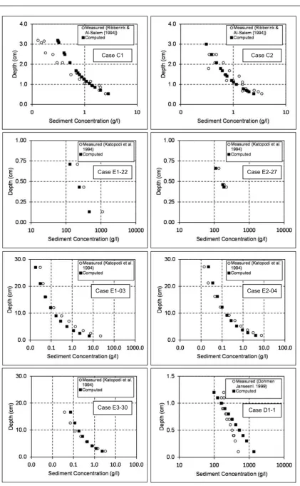
Present model of suspended sediment concentration [Eq. (22)] within suspension layer follows a power-law as initially found by Ribberink and Al-Salem [1992]. Predicted concentrations show a good agreement with the measured data. Hence Eq. (22) becomes exactly the same as the previous model of Jayaratne and Shibayama [2007].
(22) 5 . 1 * 8 . 1 * *
6
d u w A u k wc s b wc s r s
s w z d
c z
c( ) exp ( )
) ( ) 1 ( 7 d gd s k
cs
8 * k wc s s uw
M s M
s zd
Non-dimensional parameter Ms in Eq. (22) is defined as the diffusion coefficient over suspension layer. Ribberink and Al-Salem [1994] defined it as the decay parameter and specified to be a constant which was approximately equal to 2.1 for a large number of waves with uniform sand diameter of 0.21mm.
Figure 4 illustrates some examples of measured and computed results from the combined upper sheet flow (exponential) and suspension (power) models. The comparison plots shown in Jayaratne et al. [2011] are reproduced with the new numerical constants proposed in the present study.
2.2.4 Sediment suspension under breaking waves
It is a clear fact that most present models do not elucidate the terms of sediment suspension by wave breaking phenomenon. Some models try to estimate the sediment pick-up rate as a function of Shields parameter or the relative strength of shear stress acting on the seabed. However, it is doubtful if the shear stress exercises any effect on the generation of large vortices by agitation of breaking waves (Goda, 2000).
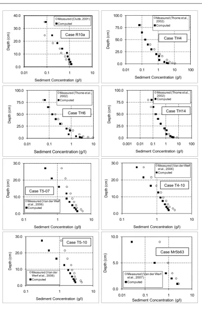
The suspended sediment concentration outside the boundary layer is likely to be determined by the entrainment and mixing due to sources such as agitation of breaking waves. Waves that plunge heavily on shallow bars or on the step of steep beaches can form very strong jets that penetrate directly to the bed and hence introduce very strong external turbulence into the boundary layer itself. These jets are also able to inject large amounts of entrained air into the boundary layer, and when this air rises, it generates large localised, upward water velocities that act as very efficient elevators for suspended sediments (Jayaratne and Shibayama, 2007). Jayaratne and Shibayama [2007] introduced the local wave orbital velocity to the bed reference equation [Eq. 23] at the location to be considered in the surf zone. Bed reference level was taken at a level of 100d from the bed (z=100d).
3 . 3 3 . 2 9 5 . 1 9 ˆ 10 ˆ ˆ s b b b w u gT u u k
c (23)
where û is the local wave orbital velocity at the location to be considered, ûb was selected as a parameter to represent the intensity of near-bottom flow at the wave breaking point (Sato et al., 1990) and k9 is a numerical constant depends on T.
Using the trial and error method, the following constants are recommended for k9 in
such a way that when 6.0sT10.0s the value of k9 is 75% from the value when T6.0s and when T10.0s the value of k9 is 75% from the value when 6.0sT 10.0s. As T increases,
wave breaking occurs at the surf zone boundary close to the offshore region and hence the magnitude of suspended sediment concentration becomes comparatively small. In other words, the value of k9 has to be decreased as X increases from the offshore boundary of the surf zone. ; 25 . 0 ; 34 . 0 ; 45 . 0 9 k
Jayaratne and Shibayama [2007] proposed diffusion coefficient (b) by incorporating
the effect of shearing force exerted on the sea bed to the eddy viscosity concept of Okayasu [1989]. z D k u k B wc b 3 / 1 11 // * 10
(24)
where k10 0.08, k11 varies from 0.0675 at wave breaking point to 0.225 at transition point (Rattanapitikon and Shibayama, 1996) as the energy dissipation takes place throughout the width of the surf zone [Eq. 25], //
*wc
u is the shear velocity under wave-current coexistent field and DB is calculated from Eq. (7).
) ( ) ( 7 . 0 3 . 0 12
11 k xxb xx
k (25)
T6.0s
6.0sT10.0s T10.0s
; T6.0s
; 6.0sT10.0s
where k12 0.225 is a constant which was assigned for spilling wave breaking condition of small-scale studies described in Jayaratne and Shibayama [2007], where x is the position in cross-shore direction and subscripts b and t denote the distances from wave breaking and transition points respectively.
The solution of concentration profile with reference level z=100d is given in the following form by Jayaratne and Shibayama [2007].
M
b zd
c z
c
100
)
( (26)
where parameter M is given by Eq. (27).
b sz w M
(27)
Figure 5 illustrates the measured and computed concentration distributions at different locations in cross-shore direction (x) with a particular time (t) from data sources of Kajima etal. [1983] and Dette and Uliczka [1986].
2.3 Mass transport velocity model
2.3.1. Vertically averaged velocity
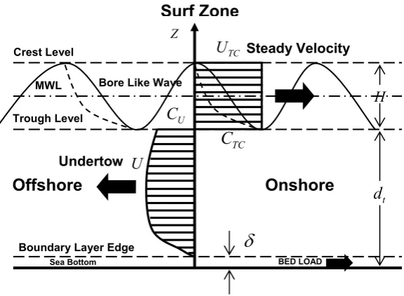
Concentration and velocity profiles throughout the water column should be predicted precisely in order to compute the on-offshore sediment transport rates. From the laboratory and field observations, it is well known that a steady drift of fluid particles is induced by the water waves in addition to the oscillatory motion both for non-breaking and breaking waves. Due to additional mass flux caused by the surface roller, the mass transport velocity induced by breaking waves generally referred to as undertow, is larger than that induced by non-breaking waves (Hansen and Svendsen, 1984).
The magnitudes of time-averaged components are usually smaller than those of oscillatory components and it has a significant effect on sediment transport. Quite a number of undertow models have been established by previous researchers, e.g. Hansen and
Offshore Zone
Inner Zone Transition Zone Svendsen [1984], Okayasu et al. [1988], Rattanapitikon and Shibayama [1996, 2000] and those models produced satisfactory results.
The main advantage of selecting the undertow model of Rattanapitikon and Shibayama [1996] for the present study is that it is capable of accurately predicting time-averaged velocity from the edge of the boundary layer to wave trough under a wide range of hydraulic parameters, as well as being applicable for various regimes in the surf zone. The vertically averaged velocity model of Rattanapitikon and Shibayama [1996] is given as follows.
h cH b
h kh H
B
Um 0.77 coth( ) 10.1
2
0 (28)
where Um is the vertically averaged velocity from the bed to wave trough caused by breaking waves, σ is the angular frequency, B0 is a parameter depends on hydraulic conditions and beach slope and expressed by Rattanapitikon and Shibayama [1996] as follows.
h H m
B0 0.1250.60 b 0.089 (29)
where mb is the bottom slope.
The constant, b1 is expressed based on the different zones in the coastal environment.
1
1 1
1 1
0
1 H Hb Ht Hb
b
where subscript b indicates the value at the breaking point and subscript t indicates the value at the transition point.
2.3.2 Width of transition zone
of the transition zone (Svendsen et al., 1978). The behaviour of the variation of wave height and mean water level inside the transition zone is quite different from the inner surf zone. Wave height decays rapidly and if mean water level is relatively constant then there is an abrupt change in slope at the transition point (Svendsen, 1984a; Basco and Yamashita, 1986). Nairn et al. [1990] used the mean water level to define the transition point. According to experiments of Okayasu et al. [1986], the abrupt change in slope could not be found. Therefore, change of wave height was a parameter to define the transition point. Basco and Yamashita [1986] defined the transition point as the point just after the rapid decay of wave height while Okayasu [1989] defined it as the point where the fully developed bore-like wave was found. From the experimental results of Okayasu et al. [1988] and Nadaoka et al. [1982], it was found that the maximum in time-averaged velocity occurs at the transition point.
By considering the above facts, Rattanapitikon and Shibayama [1996] derived the following relationship in terms of hydraulic parameters.
b ob
ot
h
h 0.8661.463
(30)
where hot is the still water depth at transition point, hob is the still water depth at breaking point and b mb Hb Lb is the surf similarity parameter at the breaking point and Lb is
the wavelength at the breaking point.
2.3.3 Vertical distribution of undertow up to wave trough
In order to analyse vertical distribution of undertow induced by breaking waves, time-averaged vertical distribution of shear stressesand eddy viscositymust be determined. Based on the dimensional analysis, Okayasu [1989] proposed a formula for computing the shear stress distribution (τ) and eddy viscosity coefficient (νt).
1/3 2/3 13 k14
d z k D
t B
Transition Zone Inner Zone Transition Zone Inner Zone where k13 and k14 are numerical constants.
The eddy viscosity coefficient can be calculated from the following formula.
z D k B t 3 / 1 15
(32)
where k15 is also a numerical constant.
Since the measured values of and t were not available, Eqs. (31) and (32) were represented
in terms of undertow velocity. Using eddy viscosity model, the undertow can be written as,
dz z U t
)( (33)
By substituting Eqs. (31) and (32) in Eq. (33), and integrating and combining with Um [Eq. (28)], finally complete undertow distribution in transition and inner zones [U(z)] is written as follows.
m t
t
B b dz dz U
D b z
U
0.22 ln 1
2 1 )
( 21/3 1/3 3 (34)
where b2 and b3 are constants and expressed as,
1 ) ( ) ( 7 . 0 3 . 0
2 b b t
x x x x b 1 ) ( ) (
3 b b t
x x x x b
In the transition zone, energy dissipation is assumed to be increased linearly from breaking point to the transition point.
2.3.4 Vertical distribution of velocity from wave trough to crest
Total sediment flux from the edge of wave boundary layer to wave trough per unit width (qsl) can be given as,
dt
sl c z U z dz
q
) ( )
where c(z) is the time-averaged concentration profile, U(z) is the time-averaged velocity profile, is the edge of the wave boundary layer and dt is the depth at wave trough.
Using the concept of mass conservation, Eq. (36) is derived to calculate mass transport velocity, UTC from wave trough to crest. Assuming that the concentration is constant throughout the wave regime and is equal to the value at the trough level given by the predictive model of suspended sediment concentration under breaking agitation, Eq. (37) is proposed to compute total sediment flux from wave trough to crest per unit width, qsu. Figure 6 illustrates definition sketch of different sediment flux layers.
dt
TC H U z dz
U
) (
1 (36)
H d c U
qsu TC ( t) (37) where U(z) is given by Eq. (34).
Table 1 and 2 show the sediment flux at different layers such as wave crest (qsu), wave trough (qsm) and the edge of the boundary layer (qsl) from Case 4.3 of Kajima et al. [1983] and Case 500 of Kraus and Larson [1988] respectively. According to simulation results, it is found that a portion of sediment mass is directed in the offshore direction due to plunging vortexes, especially close to the breaker line, while another portion is directed in the onshore direction. The mass flux at the crest level is sometimes greater than that at the level of the edge of boundary layer (Table 2). It is identified that as H (high waves) increases the mass flux also increases proportionately. From the results of Kajima et al. [1983] and Kraus and Larson [1988], it is revealed that mass flux from wave trough to wave crest has a secondary effect compared to the values at the edge of the boundary layer and wave trough. Generally, the sediment flux in this region gives a secondary effect compared to the values in the lower part of the water column.
Figure 6
2.4 Sediment transport rate formulae
2.4.1 Suspended and bed load formulae
The formulas for predicting sediment concentration and mass transport velocity described in Sections 2.3 and 2.4 are used to compute the sediment transport rate. Figure 7 illustrates the definition sketch of three-layer sediment transport model. The temporal evolution of vertical distribution of sediment concentration, c(z, t) and vertical distribution of flow velocity, us(z, t) over a wave period requires a large computation time therefore it is worthwhile to adopt more simplified forms of c(z) and us(z).
Then, the total suspended sediment transport rate from bottom to wave crest can be written as,
dz z u z c qt dt H s
s
) ( ) (
(38)
where –s is the elevation below the bottom surface where there is no effective movement of
sand particles, dt is the depth at wave trough.
Due to the difficulty in measuring the concentration and velocity accurately at the region close to and inside the moveable bed, the experimental results in those regions are very limited. Therefore, reliable formulas for predicting sediment concentration and velocity distribution have not yet been developed. In the present study, the sediment transport above the edge of the boundary layer is treated according to the time-averaged approach of sediment transport and it is referred to as suspended load. The sand transport in the lower portion is generally referred to as bed load and for the present study it is incorporated in the modified bed load formula of Watanabe [1982].
The modified bed load transport formula of Watanabe [1982] can be written in the following form.
qb Kb( c) wsd (39)
where qb is the bed load transport, Kb 2.0 (Rattanapitikon and Shibayama, 1996) and 05 . 0 c
is the critical Shields parameter.Therefore, total net sediment transport rate from bottom to wave crest can be re-written as,
b H
d
s
t c z u z dz q
q t s
) ( ) ( (40)The thickness of the boundary layer (s) is computed from the formula of Jonsson
[1966] and the roughness is computed from the formula of Nielsen [1992]. The formula of Jonsson [1966] is given as,
n b n s n s k A k
k 1.2
30 log
30
(41)
where kn is the equivalent Nikuradse roughness.
Nielsen [1992] used the measured data of Carstens et al. [1969] and Lofquist [1986] to calibrate the relationship and found the following equation for kn.
d
kn 8 170 2.5 0.05
2 (42)
where 2.5 is the grain Shields parameter using roughness equal to 2.5d.
Rattanapitikon and Shibayama [1996] proposed an explicit formula for boundary layer thickness, s, by considering Eqs. (41) and (42) using regression analysis.
0.001 26.75 33.04 5.89 26.89
8 . 0 5 . 0 n b n b n b n s k A k A k A k (43)
2.4.2 Modification to total transport rate formulae
profile change and beach profile change will feedback into the wave height transformation. Finally, the model becomes unstable and instability will be caused for long run predictions due to the high fluctuations of sediment transport rates between adjacent computation grids. Therefore, it is necessary to employ an artificial treatment or a modification to the sediment transport formula in order to control the stability of the beach deformation model.
A three-point weighted filter is applied to smooth the fluctuations of computed bed load from the modified formula of Watanabe [1982].
1 , ,
1 ,
,i 0.3 bi 0.4 bi 0.3 bi
bs q q q
q (44)
where qbs is the smoothed bed load, qb is the bed load and subscript i is the cell number. The sediment in a steep slope is expected to move in the downward direction due to gravity. Therefore, the effect of local slope is treated with the work of Watanabe et al. [1986] and Larson and Kraus [1989] by introducing an additional term, qa, to improve predictive transport rate.
x z q C
q b
bs
a
1 (45)
where C1 is the coefficient that depends on the sand diameter.
From the experience of previous researchers (e.g. Watanabe et al., 1986; Larson and Kraus, 1989; Rattanapitikon and Shibayama, 1996), C1 is selected as 10.0 for the median sand diameter (d50) less than or equal to 0.47 mm to make the model more stable. Since most natural beaches are covered with the median sand diameter of 0.20 mm, the most cases are limited to a maximum median sand diameter of 0.47 mm, which is assumed to be a good representation of most natural sandy beaches around the world.
After smoothing bed load and adding the bottom slope term into Eq. (40), the total sediment transport rate from bottom to wave crest can be expressed as,
a H
d
bs
t c z u z dz q q
q t
s
) ( )
2.5 Beach profile evolution model
2.5.1 Conservation of sediment mass
The numerical simulation model described in this section is composed of a selected wave model and sets of predictive models described in Sections 2.1-2.4. The coefficients in wave and sediment transport models are kept constant for all test cases. The beach profile change is computed from the conservation of sediment mass.
x q n t
zb t
) 1 (
1
(47)
where n is the sediment porosity, assumed to be constant along the profile.
Equation (47) is solved numerically using the Finite Difference Method (FDM). The finite difference form of Eq. (47) can be expressed as,
2 2
) 1
( 1 1
1 k tik tik tik tik i
k
i h nt x q q q q
h (48)
By simplifying Eq. (48), we have,
k ti k ti k
i k
i h nt x q q
h 1 2(1 ) 1 1
(49)
where i is the grid number and k is the time step number.
The bottom elevations at most seaward and shoreward boundaries should be specified in order to compute the bottom elevation from Eq. (49). The seaward boundary is taken as the line where there is no change in the bottom elevation and sediment can pass through the boundary. The shoreward boundary is defined at the wave run-up height and assumed to have zero change in bottom elevation. The characteristics of the swash zone are not included in the present study and the model is valid up to the end of surf zone, defined as a finite water depth close to the shoreline.
Run-up limit, ZR, is computed from the formula of Larson and Kraus [1989], by analysing experimental data of Kajima et al. [1983] and Kraus and Larson [1988].
79 . 0 0 0
47 .
1 H
where 0 mb H0 L0 is the surf similarity parameter.
To verify computed cross-shore sediment transport rates obtained by the simulation model, the rate of change of measured beach profiles can be considered. In mathematical point of view, by integrating the mass conservation equation, Eq. (47), the spatial distribution of cross-shore transport, qt(x), can be expressed as follows.
h x t h x t
dx tt t t x
q x
x
i i
i i i i
t
0
) , ( ) , ( 1
2
, 1
1
1 (51)
where x is the location in cross-shore direction, x0 is the location of no profile change, ti and
ti+1 are the time to measure profiles and h is the still water depth.
Figure 8 illustrates the definition sketch of numerical cell for computing wave height, water depth and sediment transport rate used in this study. Those three parameters are computed at the middle of the cell.
The suspended load is the dominant term describing both erosion and accretion types of beaches in the present study. The ability to predict sediment concentration formulas is limited for sand of diameter up to about 0.47 mm due to the lack of concentration measurements of coarse sand (see Table 3). Further, this resulted in using the sediment transport formula in the same range of sand diameter. For the present numerical model, cases with sand diameters up to 0.47 mm (0.18-0.47 mm) are considered including 0.20 mm case as it is the common sand diameter found in many natural beaches. Watanabe et al. [1980] reported that ripple formation and sediment suspension occurred rarely in the case of 0.7 mm sand. Therefore, for the present study, sand diameter greater than 0.69 mm is taken as zero suspended load. Due to the availability of measurements of sediment concentration for sand with diameter greater than the above-specified value (0.69 mm), the existing conditions are replaced accordingly.
Figure 8
2.5.2 Avalanching concept of Larson and Kraus [1989]
Larson and Kraus [1989] modified the avalanching concept of Allen [1970] by analysing the large wave flume data of Kajima et al. [1983] and Kraus and Larson [1988]. It was found that the repose angle (Φrp) and residual angle (Φrs) obtained by Larson and Kraus [1989] were significantly lower than that of those reported by Allen [1970]. Therefore, it was suggested to use Φrp as 280 and Φrs as 180. Further, it was also suggested to re-distribute the sediment mass
in the neighbouring grids in downward direction in such a way that the local slope was less than or equal to the residual angle, provided that local beach slope exceeded the repose angle. Initially it is assumed in the present study that avalanching takes place between cell 1 and cell 2 as shown in Fig10. In order to obtain Φrs, sand is moved between the cells. The new slope angle between cell 2 and cell 3 is checked to find out whether it exceeds Φrp. If the local slope exceeds Φrp, the computation is repeated from cell 1 to cell 3 to obtain Φrs. This procedure is continued until the local slope angle between cell N and cell N+1 is less than or equal to Φrs. Therefore, the iteration technique is employed to find out the avalanching number of cells (N) in the computation domain (Fig. 9).
Quasi-steady condition for wave field computation is used. Wave height is assumed to be unchanged during a simulating time interval, ti (ti<Δt). A simulation time interval of thirty minutes (e.g. ti=30, 60, 90, 120 min intervals due to observed field and laboratory measurements) is used in the present study. The wave height is kept unchanged during specified time interval (ti) but the sediment transport rate at each grid point is changed due to the change of the bottom slope at every time step (Δt). Since the present model requires a small computation time, i.e. 2 to 3 min to simulate 30 days beach deformation, setting up of a small time step, Δt compared to simulating time interval, ti does not cause a significant effect on the computation time. In other words, Δt remains 30 mins in most tested cases. However, if the model becomes unstable for a particular test case or dataset, the time-step, Δt (e.g. Case
K42, Δt=10 min) is further reduced in order to ensure the stability of the model and reduce the large bed deformations.
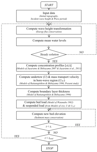
2.5.3 Model structure
The overall structure of the present beach profile evolution model is shown as a flow chart in Fig. 10. The incident wave conditions (H, T), initial bottom topography (h) and initial bottom slope (mb) are the main input parameters of the model.
3. Comparison of Simulated Results with Large-Scale and Natural Beach Data
The robustness and applicability of the beach profile model is examined by comparing initial profile (t=0 hr) and measured beach profiles at different time periods from 5 high-quality data sources of large-scale wave flume experiments and natural beaches in Japan and the Netherlands. The experimental beach profiles feature particularly offshore and onshore bars and berms, defined with respect to the initial beach profile. The beach profiles were measured at each wave run. It was reported that waves were run until beach profiles achieved to a state of equilibrium which means the particles move but there is no net sediment transport along the profile. All numerical coefficients (free parameters) in the sub models are kept constant for all test cases used in the computation. Table 4 shows the summary of data sources used in the study. Sections 3.1 and 3.2 discuss each data sources separately and model comparison results.
3.1Large-scale laboratory experiments
3.1.1 Kajima et al. [1983]
Kajima et al. [1983] measured beach profiles in a large-scale wave flume (205.0×3.4×6.0 m) at the Central Research Institute of Electrical Power Industry (CRIEPI) of Japan in 1981. The total number of test cases performed by Kajima et al. [1983] is 19 and all cases started with a
Figure 10
uniform initial beach slope, ranging from 1/50 to 1/10. The highest measured storm duration is t=60 hr (2.5 days). Most numerical results (e.g. Test Case 1.1, 1.2, 1.3, 1.4, 1.5, 1.6, 1.7, 3.1, 3.2, 3.3, 3.4, 4.1, 4.2, 4.3, 4.4, 5.1 and 6.1) show good agreement with the general trend of the measured beach profile from offshore to onshore, illustrating main morphological features such as sand bars and berm formation. This means that evolution of bars and berms were found to be regular under steady wave and gradually varying water depth. Some test cases such as Case 3.3, 3.4, 4.2, 4.3 and 6.1 illustrate shifting of the large sand bar towards onshore and this could result in shifting of the predicted breaker line. Predicted results of Case 4.4 and 5.2 show greater beach deformation as the storm duration increases (e.g. Case 4.4 at t=10 hr and Case 5.2 at t=60 hr). One of the reasons for this discrepancy may be the non-conserved sediment mass in the cross-shore profile and perhaps it was not captured by the 2D model. Figures 11-20 represent the measured and computed beach profiles at equilibrium state. Table 5 shows the details of each test case used in the study.
3.1.2 Kraus and Larson [1988]
Kraus and Larson [1988] reported beach profile changes in a large wave flume (193.5×4.6×6.1 m) at the Coastal Engineering Research Centre (CERC) of the US Army Corps of Engineers Waterways Experiment Station, which were measured in 1956-1957 and 1962. The total number of test cases carried out by Kraus and Larson [1988] is 12 and two tests were performed with an irregular initial beach slope. The highest storm duration considered under these tests were t=40.5 hr. Generally, the computed profiles show the same tendency as the measured profile at equilibrium state (e.g. KL101, KL200, KL400, KL510, KL600, KL610, KL700). Cases with extreme wave conditions such as Case KL100, KL300, KL500 and KL700 show some undulating nature at crest and trough of sand bar and erosion in the onshore and the reason might be the sudden deposition of sediment by gravity before suspension occurs. A sharp-crested offshore dune and an onshore sand bar are formed in Case
KL510 and this can be due to the presence of irregular initial beach slope. The computed results of Case KL100, KL200, KL500 and KL700 illustrate shifting of the sand bar towards onshore region compared to the measured shape. The main cause is identified as the shifting of the predicted beaker line. Further, it is observed from Case KL100, KL101, KL300 and KL700 that they were performed under long period and high waves. Similar to Kajima et al.
[1983] , it is found from the computed results that the longer the simulation time the larger the instability of the model results due to the greater deformation of beach topography (e.g. KL300 t=20 hr, KL700 t=15 hr). In other words, smaller the wave climate (both smaller H
and T and either smaller H or smaller T) better the comparisons results are (e.g. KL510, KL600 and KL610). Figures 21-25 show the measured and computed beach profiles at equilibrium state. Table 6 shows the details of test cases used in the study.
3.2 Field measurements
3.2.1 PARI data [2005, 2009]
The Port and Airport Research Institute (PARI) of Japan owns the Hazaki Oceanographic Research Station (HORS). HORS operates a research pier of 427 m long on the sandy beach facing to the Pacific Ocean. This pier captures the waves in the surf zone, between wave breaking point and the limit of wave up-rush on the beach, where a large amount of sediment is transported by wave action and wave-induced nearshore currents. Beach profiles from the tip of the pier to the backshore are measured with intervals of 5.0 m daily. Table 7 shows the details of both non-storm and storm test cases used in the present study.
a) Non-storm conditions [2005]:
Under non-storm conditions, the predicted and measured beach profiles including inner and offshore bar migration and trough deepening (x<450 m) at Hazaki coast match very well at
t=24 hr (1 day) to t=240 hr (10 days). Since the swash dynamics are not included in the
present model, the predicted profiles in the upper part of the swash zone (x≤75.0 m) show an average beach slope. It was observed from the predicted results that the bar migration and trough deepening at t=720 hr (30 days) has shifted towards onshore due to the change of breaker line and weakening of wave attack in that area (less energetic conditions).
There are several possible factors affecting the estimation of topography (water depths). As the water depth becomes shallower towards the beach, the effect of non-linearity in wave behaviour become more significant, causing higher wave celerity than the linear theory predicts and hence causing an over estimate of water depths [Bell, 1999]. The influence of currents, both tidal and wave induced, are also a potential source of variability in topography estimation. Such currents make the derived water depths larger if the current is in the direction of wave motion or smaller if the current is in opposition to the waves [Bell et al., 2004]. In general, the present model shows very good agreement with the measured beach profiles up to t=240 hr (10 days) and some discrepancies when t>240 hr (e.g. t=720 hr), but simulated results are reasonably acceptable which may be due to a coincidental cancelling of probable effects from different factors. Figure 26 shows the measured and computed beach profiles at t=24-720 hr.
b) Storm conditions [2009]:
The measured beach profiles at Hazaki coastal under storm conditions in 2009 illustrate that a bar located fairly close to the shore may contain crescentic structures (see e.g. Case 1, 4 and 5) that are diminished during storms while a bar located further offshore is generally alongshore uniform (see e.g. Case 4, 5, 6). Cases 1, 2 and 4 were recorded with high wave action. In Case 1, the predicted profile at t=24 hr shows two nearshore peaks (around x=250, 300 m) and large deformation in the offshore region after x=375 m. When t=72 hr and t=96 hr, simulated profiles show more deposition than measured offshore bars (x=275-350 m) and in some point (x=350-375 m) both profiles match each other before deposition takes place
![Fig. 5. Measured and computed suspended sediment concentration profiles under field-scale breaking agitation from Jayaratne & Shibayama [2007]](https://thumb-us.123doks.com/thumbv2/123dok_us/426674.1042329/56.595.110.516.60.560/measured-computed-suspended-sediment-concentration-agitation-jayaratne-shibayama.webp)
![Fig. 9. Definition sketch of avalanching concept of Larson & Kraus [1989].](https://thumb-us.123doks.com/thumbv2/123dok_us/426674.1042329/58.595.114.546.73.372/fig-definition-sketch-avalanching-concept-larson-kraus.webp)
![Fig. 11. Measured and computed beach profiles from Kajima et al. [1983], Case 1.1 & 1.2](https://thumb-us.123doks.com/thumbv2/123dok_us/426674.1042329/60.595.59.537.87.482/fig-measured-computed-beach-profiles-kajima-et-case.webp)
![Fig. 12. Measured and computed beach profiles from Kajima et al. [1983], Case 1.3.](https://thumb-us.123doks.com/thumbv2/123dok_us/426674.1042329/61.595.60.541.86.418/fig-measured-computed-beach-profiles-kajima-et-case.webp)
![Fig. 13. Measured and computed beach profiles from Kajima et al. [1983], Case 1.4 & 1.5](https://thumb-us.123doks.com/thumbv2/123dok_us/426674.1042329/62.595.58.538.83.747/fig-measured-computed-beach-profiles-kajima-et-case.webp)
![Fig. 14. Measured and computed beach profiles from Kajima et al. [1983], Case 1.6 & 1.7](https://thumb-us.123doks.com/thumbv2/123dok_us/426674.1042329/63.595.65.543.62.764/fig-measured-computed-beach-profiles-kajima-et-case.webp)
