Base Drag Considerations and Projectile Optimization on 0 5 caliber Projectile

Base Drag Considerations and Projectile Optimization on 0.5-Caliber

Projectile

Byregowda G.

Department of Aeronautical Engineering

ACS College of Engineering, Bangalore-560074, India

Abstract— One of the most important aerodynamic

performance characteristics for the projectiles is the total drag. The total drag for projectiles can be divided into pressure drag (excluding the base), viscous (skin friction) drag, and base drag. The base drag is a major contributor to the total drag, particularly at transonic speeds. Thus, the determination and minimization of base drag is essential in minimizing the total drag of projectiles. This Information can aid the designer to find potential areas for drag reduction and achieve a desired increase in range and/or terminal velocity of projectiles since they are affected by the projectile drag. Improved projectile performance can be achieved in several different ways up to a certain extent, and can be combined in one and the same projectile. Base drag contributes generally to a relatively large part of the total drag and depends upon the fact that the base pressure due to the resulting wake flow in the base region is lower than the ambient air pressure. Current project deals with utilization of this phenomenon for overall reduction of total drag.

Key words: Base Drag Considerations, Projectile

Optimization, 0.5-Caliber Projectile

I. INTRODUCTION

A number of conditions can cause standard munitions such as mortars and artillery to miss an intended target. These conditions include variable atmospheric conditions, firing platform motion, aiming errors, and manufacturing inaccuracies of the gun-tube, propellant, and projectile. With the advent of smart weapons technologies, guided munitions can be used to dramatically lower dispersion error and collateral damage; however, development of these guided projectiles has presented weapons designers with numerous complex technical challenges over the past several decades. Control mechanisms and onboard electronics suites must be small due to size limitations and rugged to withstand extreme acceleration loads and high spin rates. Furthermore, guided projectiles are often fired in large quantities and therefore must be relatively inexpensive to produce. To reduce cost, smart weapons developers have now begun to investigate more unconventional guided projectile concepts with passive roll control capability.

II. PROJECTILE LINEAR THEORY

Projectile Linear Theory has long been an analytical work horse in the ballistics community and is used to reduce the complexity of the flight dynamic equations of motion through application of a series of simplifications and assumptions. These linearized equations of motion allow the engineer to apply concepts from Linear Systems Theory, which is well understood and easily implemented. Over time, projectile linear theory has been used for stability analysis, aerodynamic coefficient estimation using range data and fast trajectory prediction. Basic projectile linear theory has

extended by various authors to handle more sophisticated aerodynamic models, asymmetric mass properties, fluid payloads moving internal parts dual spin projectiles, extending flight, lateral force impulses and model predictive control. Recently, an extended linear theory for aerodynamically asymmetric lifting surfaces has been developed for a specific canard configuration to investigate the effects of canard dithering and canard stall on projectile roll and pitch damping.

III. LITERATURE REVIEW

1) Sidra I. Silton and Surya P.G. Dinavahi conducted a study on “BASE DRAG CONSIDERATIONS OF 0.5-CALIBER SPINNING PROJECTILE”. According to their study the computed base pressure in the subsonic and transonic flight regimes were found to be quite larger (sometimes even greater than free stream) such that either a very small or negative bases drag was observed. Their study investigated the cause of this phenomenon by investigating the flow in the subsonic and transonic regimes at zero angle of attack. They have conducted computations on the standard 0.5-cal geometry were conducted using multiple turbulence models, multiple computational meshes, and multiple flow solvers to validate that this is not a numerical phenomenon. Additionally, the effect of boattail and base geometry on the base drag was investigated in order to better understanding the flow phenomenon leading to the reduced base drag.

2) Kiran Torangatti, and Dr.Basawaraj,. had conducted an

research on “DRAG PREDICTION AND

body and details of the mesh is given below for the domain. No. of nodes – 1,10,751 and No. of elements – 1,10,000 Mesh quality Orthogonal quality of mesh ranges from 0 to 1. Where values close to zero corresponds to low quality Minimum Orthogonal Quality – 0.833129579949384 Maximum Aspect Ratio – 223.679 The following boundary conditions, solving models and schemes are used in post processing procedure using the above mesh details and with quality of the 2D mesh model. Turbulence model with realizable enhanced wall functions as it is a related to the projectile outer surface and domain top wall surface and the reason behind using this model is that, we have not considered the y+ wall functions as in that case we should use k- turbulence model. Explicit scheme is used in solving the solution.

3) M.E. Wessam, and Z.H. Chen, had conducted a project on “FLOW FIELD INVESTIGATIONS AND

AERODYNAMIC CHARACTERISTICS OF

ARTILLERY PROJECTILE”. Their paper describes a computational study to determine the aerodynamic coefficients at subsonic and supersonic speeds using an unstructured flow solver. The paper presents results of investigation of a flow over 155 mm artillery projectile M107 and the performance of the ANSYS FLUENT computational code. The flow around projectile was solved as 3-D unsteady compressible flow. And the model used for their investigation was Spalart-Allmaras turbulent model. The convective term is approximated by second order Roe-FDS scheme. The second order central difference scheme is applied to pursuing numerical approximation of the viscous term. Runge Kutta method was applied to step on time. For Spalart-Allmaras model. 4) Bradley E. Howell, Sidra I. Silton and Paul Weinacht had conducted an project on “THE EFFECT OF BOATTAIL GEOMETRY ON THE YAW LIMIT CYCLE OF

SMALL CALIBER PROJECTILES”. Their

experimental test describes the design to determine the effects of boattail angle and radius on the yaw limit cycle. Their test created a design space in which to begin determining the effect of aft projectile geometry on both the aerodynamic coefficients and yaw limit cycle. The design space was limited to the geometry of the intersection between the boattail and base of the projectile and the boattail angle. A more detailed design space including boattail length should be investigated prior to any definitive conclusions being drawn. A more expansive Mach number range could also be investigated. The results indicate a significant change in yaw behaviour can be affected only by changing the intersection between the boattail and the base of the projectile – varying the boattail angle has a negligible effect on the yaw limit cycle. The presence of a chamfer and variation of boattail angle over the limited range investigated has minimal effect on the yaw limit cycle of the projectile. Each variant fired indicated that a limit-cycle does exist at the Mach numbers investigated and that it continues to increase with decreasing velocity. It appears that a sharp intersection between the boattail and base minimizes the yaw limit cycle, both in delaying the onset of occurrence as well as minimizing the angle.

5) Variganji Sanjeev Kumar, has carried a study on “ESTIMATION OF BASE DRAG ON SUPERSONIC CRUISE MISSILE”. Their intention of finding the base drag on a supersonic cruise missile was to study the variation of aerodynamic parameters which change with altitude, also to make sure that the coefficient of drag on the base through the Brazzel's technique, which used a MATLAB code, is analogous to the results from a CFD analysis through FLUENT. They have been found that the results in both the methods are more or less equal to each other with an average of 5.3% as the percentage error while comparing both the methods. Hence, it can be concluded that, based on the results and comparisons, the Base drag coefficient decreases with increase in altitude and Mach number and that the missile's performance is increased during cruise at a higher exit Mach number and a higher altitude where ambient pressure is reduced relieving the jet's plume to expand more and reduce air recirculation at the base.

6) Abdulkareem Sh. Mahdi Al-Obaidi has conducted study on “EFFECT OF BODY SHAPE ON THE

AERODYNAMICS OF PROJECTILES AT

SUPERSONIC SPEEDS”. He has done an investigation which has been made to predict the effects of forebody and afterbody shapes on the aerodynamic characteristics of several projectile bodies at supersonic speeds using analytical methods combined with semi-empirical design curves. The considered projectile bodies had a length-to-diameter ratio of 6.67 and included three variations of forebody shape and three variations of afterbody shape. The results, which are verified by comparison with available experimental data, indicated that the lowest drag was achieved with a cone-cylinder at the considered Mach number range. It is also shown that the drag can be reduced by boattailing the afterbody. The centre-of-pressure assumed a slightly rearward location for the ogive-cylinder configuration when compared to the configuration with boattailed afterbody where it was the most forward. With the exception of the boattailed afterbody, all the bodies indicated inherent static stability above Mach number 2 for a centre-of-gravity location at about 40% from the body nose.

for minimum drag can be applied on similar flying bodies. Their solution was done by using two dimensional axisymmetric pressure based solver with Splart Allmaras viscous model, the pressure and velocity equations have been solved coupled and implicit using second order discretization. The wall Y+ values were maintained in the range of (30-60) for most cases. The solution accuracy depend on stopping iterations if there is no change in drag coefficient up to 5th digit within more than 500 iterations.

IV. PROBLEM STATEMENT

Current study of this project involves CFD analysis over a standard 0.5-caliber projectile which is taken from Ref [1] modifying a base taper angle (Boattail angle) and base taper length (Boattail length) without modifying actual size (overall length and body radius) there by optimizing a bullet design for any particular flight regime. The optimizing any particular projectile involves two major possible ways.

A. Reducing Overall Drag (Cd)

This can be accompanied by modifying the projectile aerodynamically with suitable optimum design, hence to reduce overall Cd (drag co-efficient).

B. Optimizing Base drag (Cd Base)

Base drag is a negative component of overall drag which acts in the same direction as of projectile’s velocity direction. So increase of this negative component of base drag can reduce overall drag, this can be done by modifying base region of the projectile with optimum Boattail angle, Boattail length and base fillet.

V. PROJECT OBJECTIVES & SCOPE

 The CFD analysis has made significant progress in simulating the effects of Transonic and supersonic flows over the spinning projectile and the objective of the present study is to model the flow physics of base side of the projectile and to arrive at an optimum projectile design for which base drag is minimum.

 To predict the pressure, velocity and viscosity distribution over a surface of projectile using commercially available CFD packages such as ANSYS ICEM CFD and ANSYS FLUENT.

 To validate CFD results against existing literature results.

 Study of this project involves base drag and drag optimization which can be even applicable for missile designs.

VI. DESIGN PARAMETERS

Design parameters for the projectile design are taken from Ref [1] which is standard 0.5-caliber radius with 1.756-caliber overall length. Boattail modification for this standard projectile is done by two parameters, which are

 Boattail length ( Lbt ) and

 Boattail angle (θbt).

As per Ref [1] the boattail angle and boattail length are considered as a design variable since experiments have

shown that body drag decreases approximately linearly with increasing the boattail length. Appreciable reduction in base drag can be obtained with boattails of moderate angles and lengths. An optimum boattail configuration results from balancing the increase in wave drag with the reduction of base drag.

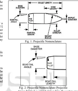
Fig. 1: Projectile Nomenclature

Fig. 2: Projectile Nomenclature Projectile

Using boattail is intended to reduce the vortex area behind the base, so the strong vortex will be replaced by a smaller and a weaker one.Hence the modification is done only on rare side of the bullet as shown in above figure without varying nose length, secant radius, meplat diameter and standard radius and length. Several standard models which are obtained by varying by Boattail angle (θbt) and Boattail length (Lbt) are considered from Ref [1].

A. Meshing

In computational solutions of partial differential equations, meshing is a discrete representation of the geometry that is involved in the problem. Essentially, it partitions space into

elements (or cells or zones) over which the equations can be approximated. Zone boundaries can be free to create computationally best shaped zones, or they can be fixed to represent internal or external boundaries within a model.

VII. ANSYSICEMCFD14.5

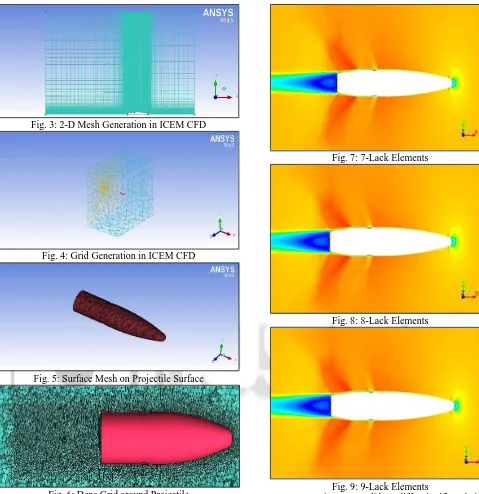
Fig. 3: 2-D Mesh Generation in ICEM CFD

Fig. 4: Grid Generation in ICEM CFD

Fig. 5: Surface Mesh on Projectile Surface

Fig. 6: Dens Grid around Projectile

A. Grid Independence Study

As can be expected, results obtained by numerical calculations were sensitive to grid points; the point at which the results do not vary with number of grid points is accepted to give independent results. Results obtained varies gives accurate results with the finger grid size, so the final grid size chosen depends on the accuracy of the results, available resource and the level of accuracy required for designer. Here we have done the analysis on 7lack 8lack and 9lack grids. The distortion in the contours of

Fig. 7: 7-Lack Elements

Fig. 8: 8-Lack Elements

Fig. 9: 9-Lack Elements

Dynamic pressure did not differ significantly in both 7lack and 8lack grids. In order to ensure the absence of solution distortion analysis over 9lack grid was carried out. In the grid independent study 0.78-caliber 9o _{base radius} model was used, with a sonic flow velocity and with 101325pascal pressure and 300K as standard temperature. Density based solver with a flow model k-e (Realizable) with second order upwind was used along with solution steering. Above Figure shows the corresponding contours obtained.

B. Boundary Conditions

The governing equation of fluid motion may result in a solution when the boundary conditions and the initial conditions are specified. The form of the boundary conditions that is required by any partial differential equation depends on the equation itself and the way that it has been discretized. The CFD simulation was run using FLUENT 14.5. The boundary conditions assigned for the simulation were taken

Sl.no Parameters

Sub-Parameters

Boundary Conditions

1 General

Parameters

Solver-Type Density Based Velocity

Formulation

Absolute

Gravity Not

Considered

2

Viscous Model Type

(k-ε model)

k-ε model type Realizable

Near wall

treatment

Standard Wall Functions Model

Constants

Fluent default values User-Defined

Functions

None

3 Flow Fluid

(Air)

Density Ideal-Gas

(kg/m3₎ Specific Heat

(Cp)

1006.43 (j/kg-k)

Thermal Conductivity

0.0242 (w/m-k)

Viscosity 1.7894e-05

(kg/m-s) Molecular

Weight

28.966 (kg/kgmol)

4

Pressure-Far-Field

Pressure 101325

Pascal

Temperature 300K

Mach Number 0.6 to 2

5 Outlet Pressure 101325

Pascal

Temperature 300K

6 Solution

Methods

Formulation Implicit

Flux-Type Roe-FDS

7

Spatial Discretization

Gradient Type Least Squares Cell Based

Flow Type Second Order

Upwind Turbulent

Kinetic Energy

Second Order Upwind Turbulent

Dissipation Rate

Second Order Upwind Initialization

Method

Standard

8 Solution

Initialization

Compute from Pressure-Far-Field

Flow Type Subsonic,

Transonic, Supersonic

9 Solution

Steering

First to Higher Order Blending 100% FMG Initialization Yes Boundary Conditions Defined in FLUENT 14.5

Table 1:

From Ref [1]. The standard k-ε realizable with standard wall function was used which is well suited for turbulence problem. Density based solver is used since the analysis involves subsonic, transonic and supersonic flows. Whereas pressure based solver is preferred only for incompressible flows and some part of low speed subsonic flows. Steady state condition is used since it is a time independent analysis. Air with ideal gas condition is used as a flow fluid with default values of specific heat conductivity, Thermal conductivity, Viscosity and Molecular weight. In cell zone conditions operating condition is set to zero Pascal. Pressure-far-field is defined by selecting all the surfaces except outlet surface. Velocity-inlet is not preferred since it affects the accuracy of results for incompressible flows. Both inlet and outlet are given with a standard atmospheric pressure of 101325 Pascal. Cartesian co-ordinate system is selected since all the analysis over all the models is done at zero angle of attack and the model is aligned in positive x direction x-component of flow velocity is given as negative one. And rest all velocity components are maintained at zero. Mach number is varied from subsonic region to supersonic region for all configurations of projectile models. Both

turbulent intensity and viscosity is maintained at their default values in the solver. At reference value section under the compute from drop-down list Pressure-far-field is selected.

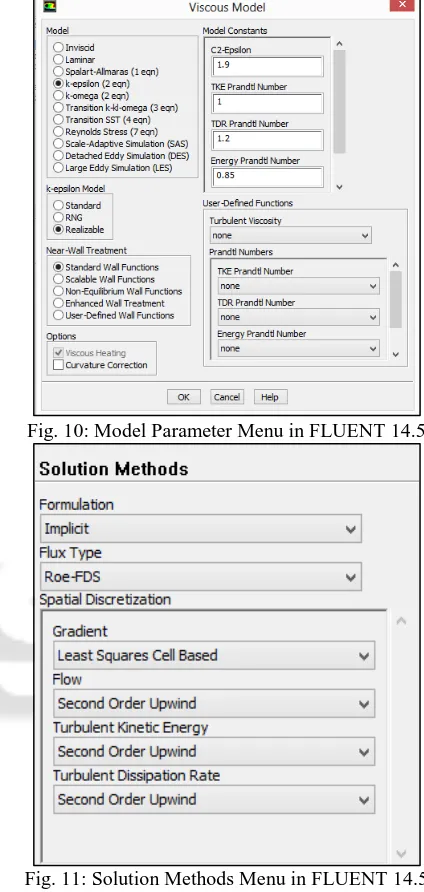
Fig. 10: Model Parameter Menu in FLUENT 14.5

Fig. 11: Solution Methods Menu in FLUENT 14.5 Under solution methods implicit formulation with Roe-FDS as a flux type is selected. And in spatial discretization for gradient least square cells based method and for the flow, turbulent kinetic energy and turbulent dissipation rate second order upwind method is used. Insolution control menu lower values of under-relaxation were used for turbulent kinetic energy, Turbulent Dissipation rate and for turbulent viscosity. Lower values of under-relaxation factors helps to keep the solutions without divergence. Solution initialization is done by standard method by selecting pressure-far-field as reference values. Solution steering is activated in order to automatically assign the courant number. The above table shows the detailed Boundary conditions which is applied to all projectile configurations.

C. Solving

generated projectile models are imported and Boundary Conditions are defined as per table in previous page. And then standard solution initialization is done. Solution iterations are carried out until the stabilized results are obtained as per grid decency study. All the simulations were performed in parallel on system having 2.3Ghz i3 processor. The steady state calculations took approximately 7-8 seconds of CPU time per iteration.

D. Results & Discussions

The computational study for the projectile has been carried out through various techniques using k-ε turbulent model. This was the turbulent model of choice as it had previously been found to give good results across the Mach number range of interest (Mach 0.6 to Mach 2) for all aerodynamic coefficients. Using the two equation turbulent model, it was discovered that the base component of the drag coefficient’s CD, was negative at zero degrees angle of attack for all Mach numbers below Mach 0.94. Additionally, at Mach 0.98, although the base drag contribution, CDbase was positive it was very small.

E. Confirmation of Negative Base Drag

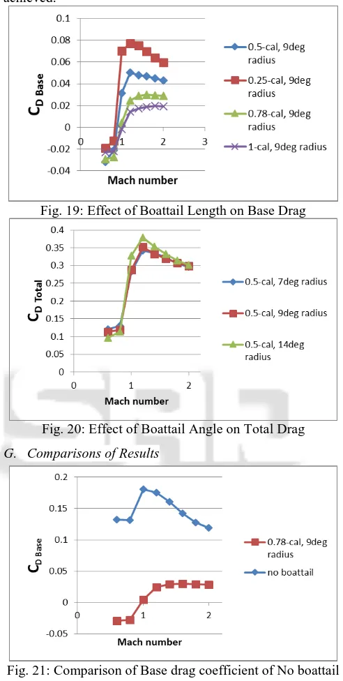
Upon discovery of this negative base drag phenomenon, the plots of CDbase versus Mach number for all configurations of projectiles are plotted. It seen that negative base drag was not a computational issue from Ref [1]. By knowing this phenomenon we considered this Negative base drag to optimize the projectile models. And it is occurring regardless of mesh and other parameters. While base drag is not affected by the other parameters except the radius between the boattail and base, the boattail length, and the boattail angle. Reducing the magnitude of any of these parameters from their normal values appears to increase the base drag contribution. An increase in boattail length showed a decrease to the base drag contribution consistent with what was expected. An increase in boattail angle, however, was not consistent with the trends most likely due to flow separation, especially at subsonic Mach numbers.

Fig. 12:

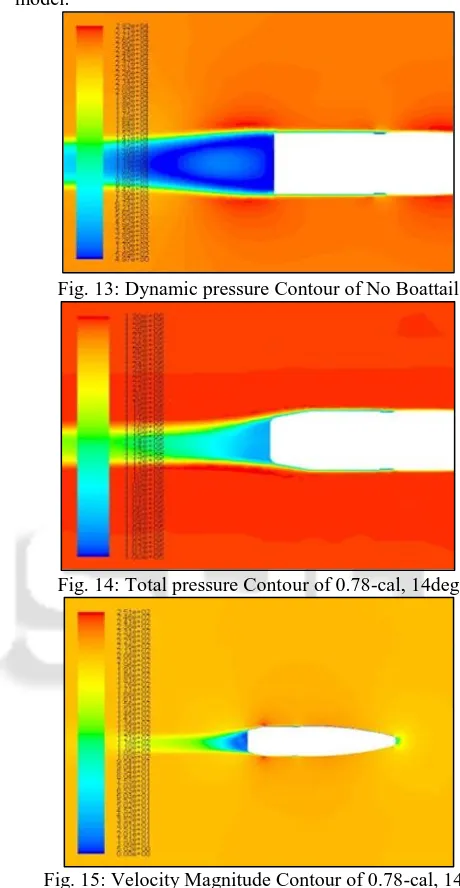
In order to visualize the phenomena of base drag of base drag several contours are shown in next section. And they are discussed in detail with suitable plots. As in case of No boattail projectile model this negative base drag phenomena is not seen, since the No boattail projectile doesn’t contains any tapper section, boattail angle and base radius.

To visualize the formation of negative base drag several contours like Dynamic pressure, Total pressure and Velocity contours of all projectile models are generated and are compared with the contours of No boattail projectile model.

Fig. 13: Dynamic pressure Contour of No Boattail

Fig. 14: Total pressure Contour of 0.78-cal, 14deg

F. Discussions on Results Obtained

After solving for the results the data’s are collected for each and every projectile model, compression of each and every results of projectile models as per Ref [1], plotting the graph of CD Total versus Mach number as shown in below figure.

Fig. 16: Graph of Total drag coefficient versus with Mach number

After plotting the results it is found that coefficient of total drag (CD Total) was having least values for 0.78-cal 9o radius projectile model. Further in order to determine the effects of variations of geometrical parameters such as boattail length, boattail angle and base radius. Individual graph is plotted keeping one geometrical parameter as constant and varying the other parameters, i.e. variation of results with respect to boattail angle can determined by selecting a projectile models having constant boattail length. And variation of results with base radius can be determined by plotting the results for no base radius and base radius for any particular projectile model with same boattail length and boattail angle. And the effect of boattail length can be determined by plotting the results for one particular boattail angle and base radius.

Fig. 17: Effect of Base Radius on Base Drag

Fig. 18: Effect of Boattail Angle on Base Drag

The optimization of projectile design is seen from comparison of results. Hence the results of optimized model 0.78-caliber 9o _{with base radius are compared with the No} Boattail model in order to know the amount of optimization achieved.

Fig. 19: Effect of Boattail Length on Base Drag

Fig. 20: Effect of Boattail Angle on Total Drag

G. Comparisons of Results

Fig. 21: Comparison of Base drag coefficient of No boattail and 0.78-cal 9o Radius Projectiles

The optimization of projectile design is seen from comparison of results. Hence the results of optimized model 0.78-caliber 9o _{with base radius are compared with the No} Boattail model in order to know the amount of optimization achieved.

VIII. CONCLUSIONS

After comparison of No-boattail projectile models result and 0.78-cal 90 _{Radius projectile models result near Mach number} 0.6, it if found that 0.78-cal 90 _{Radius projectile model was} having 46 percentage of reduction of total drag as compared to No-boattail model. And at transonic Mach number 1 it was found that 0.78-cal 90 _{Radius projectile model was having 12} percentage of reduction of total drag as compared to No-boattail model. And at higher supersonic Mach number 2 it was found that 0.78-cal 90 _{Radius projectile model was} having 7 percentage of reduction of total drag as compared to No-boattail model. In which these values are comparable with the Ref [7], And the phenomena which is causing complete reduction of total drag near subsonic flow Mach number was found to be the negative contribution of base drag. Near subsonic flow regimes these base drag was found to be contributing higher reduction of total drag as per Ref [1]. Hence by utilizing these phenomena and considering base drag as main parameter the projectile optimization of 0.5-cal is carried out.

IX. FUTURE WORK

 The present work will give the idea about total drag and further analysis will give the better design results which can be carried out for future work.

 By implementing the proper design in shell section in rare section of the projectile model further optimizes the result properties.

 Future studies on powered projectiles (Missiles, Rockets, Powered bullets etc.) will give the idea over a reduction of base drag by expelling hot gases.

REFERENCES

[1] Sidra I. Silton U.S. Army Research Laboratory, Aberdeen, MD, 21015 and Surya P.G. Dinavahi University of Alabama at Birmingham, Birmingham, AL 35294.

[2] Kiran Torangatti, 1Research Scholar, Department of Aerospace Propulsion and Technology, VTU-CPGS Bangalore -560018, Karnataka, India and Dr.Basawaraj, Associate. Professor, Department of Aerospace Propulsion and Technology, VTU-CPGS Bangalore- 560018.Karnataka, India.

[3] M.E. Wessam, Key Laboratory of Transient Physics Nanjing University of Science & Technology Nanjing, China and Z.H. Chen, Key Laboratory of Transient Physics Nanjing University of Science & Technology Nanjing, China.

[4] Bradley E. Howell, Data Matrix Solutions, Aberdeen Proving Ground, MD 21005-5066 Sidra I. Silton and Paul Weinacht, Weapons and Materials Research Directorate, ARL, Aberdeen Proving Ground, MD 21005-5066.

[5] Variganji Sanjeev Kumar, PG Student, Department of Aerospace, Marri Laxman Reddy Inst of Tech & Mang, Hyderabad, Telangana, India.

[6] Abdulkareem Sh. Mahdi Al-Obaidi School of Engineering, Taylor’s University College, No 1 Jalan SS 15/8 47500 Subang Jaya, Selangor DE, Malaysia. [7] M. A. Suliman, O. K. Mahmoud, M. A. Al-Sanabawy,

O. E. Abdel-HamidPaper: ASAT-13-FM-05.

[8] Krieger, R. J. and Vukelich, S. R., "Tactical missile drag, tactical missile aerodynamics", Prog. Astronautics Aeronautics, AIAA 104, 383-420. (1986).

[9] J.Sahu, “Drag Predictions for Projectiles at Transonic and Supersonic Speeds,” US Army Ballistics Research Laboratory, Aberdeen Proving Ground, MD, BRL- MR-3523, June 1986.