Independence of Mean Squares in Unbalanced Nested Designs

(1)

(2)

Independence of Mean Squares in Unbalanced

Nested Designs

Dr.W.S.Brar1

1

PG Department of Mathematics Baba Farid college Baba Farid Group of Institutions Bathinda -151001 , Punjab, India

Abstract: In this paper, the distributional properties of independence of mean squares in three stage unbalanced nested designs with random effects have been investigated. The correlation coefficients between mean squares of main classes and mean squares of subclasses of different design structures have been calculated. Also the condones have been derived under which mean squares of main classes and mean squares of sub classes are independently distributed

Keywords: unbalanced, nested, mean squares, independence, correlations , designs

I. INTRODUCTION AND LITERATURE SURVEY

In balanced three stage nested classifications with random effects, the mean squares in the analysis of variance are independent and are chi-squares distributed under the usual normality assumptions. The variance component estimators are linear functions of mean squares and their variances can be derived accordingly. When the classification data are not balanced, the mean squares , in general , are no longer independent and also they do not follow chi-square type distributions. Similarly the distributions of variance component estimators of classes and subclasses are not linear combinations of chi-squares in unbalanced classification. An exact test does not always exist even in balanced designs for random effects model. The ANOVA testing procedures were extended by [1], [2] and [3] for the construction of approximate F-tests in unbalanced designs. These tests make use of the fact that the mean squares are distributed independently and have chi-square type distributions but that do not generally hold for unbalanced designs. Ignoring all these factors, onle appromate tests developed for balanced designs have also been applied to unbalanced designs. [4] have discussed approximate F-tests for testing the variance components in which correlation of mean squares of numerator and synthesized denominator of F- test are calculated. Further, they have calculated correlations of mean squares in some special cases. There is a need to study the dependence of mean squares on all types of imbalance in nested designs. Further, [6] has mentioned that zero covariance of mean squares always implies independence under the normality assumptions. Therefore , an empirical study of twenty designs of different structures is undertaken and calculated the correlations and derived the conditions under which the mean squares are independently distributed. Consider the three stage unbalanced nested random effects model :

=µ+ + +

i=1,2,…..a , j=1,2,…... . k= 1,2,………….

Where yijk is the observation, µ is the general mean, ai and bij are the random effects, eijkthe random error associated with yijk. As usual, it is assumed that ~ (0, ) , ~ (0, ), ~ (0, )

The ANOVA for three stage unbalanced nested design with random effects is given in Table 1 below :

Table 1

Analysis of Variance (ANOVA)

Source of variation d.f Mean Squares Expected Mean Squares

Main classes f3 y’Q3y/f3 =V3 + +

(3)

Within subclassesf1 y’Q1y /f1 =V1

Where

Q3 = ∑ − / , Q2 = ∑ ∑ / - ∑ , Q1 = I - ∑ ∑ /

q0 = ∑ ∑ ( 1/ −1/ ) /f2 , q1 = ∑ ∑ ( 1/ −1/ ) /f3 , q2 = ∑ ( 1/ −1/ ) /f3

also ∑ = , ∑ = , ∑ ∑ = ∑ =

f1 =n - ∑ f2 = ∑ − f3 = a – 1

The row vector ′ of yijk ‘ s is ′ = , ,… … … … . ; ′ … … …

And Jn is the × matrix of 1’s and ∑ is the direct sum of matrices A1 , A2 ………..Ak as defined in [6].

[image:3.612.38.532.78.298.2]

The designs are given below in Table 1.

Table 1

1 2 3 4 5 6 7 8

Design1 bi 2 2 2 2 a=4

nij 2,1 2,1 2,1 2,1

Design2 bi 2 2 2 2 2 2 2 2 a=8

nij 2,1 2,1 2,1 2,1 2,1 2,1 2,1 2,1

nij 20,1 20,1 20,1 20,1

nij 2,2 2,2,2 2,2 2

nij 3,3 3,3,3 3,3 3

nij 2,2,2,2,2 2,2,2,2 2,2 2,2,2,2,2,2,2

Design7 bi 15 2 1 a=3

nij 2,2,2,2,2,2,2,2, 2,2,2,2,2,2,2

2,2 2

Design8 bi 2 1 1 1 1 a=5

nij 4,4 2 2 2 2

nij 4 3,3 2,2,2 1,1,1,1

Design10 bi 3 4 2 3 2 a=5

nij 4,4,4 2,2,2,2 1,1 3,3,3 5,5

Design11 bi 2 2 2 2 1 1 a=6

nij 2,2 1,1 1,1 1,1 1 1

Design12 bi 2 2 2 2 1 1 a=6

(4)

Where ‘a ‘ indicates the number of main classes, bi indicates the number of subclasses within the main class and nij the number of observations.

II. RESULTS AND DISCUSSION

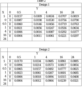
Correlations between V2 and V3 in three stage unbalanced nested designs are given in Table 2 :

Table 2 Design 1 X ↓ 0 0.5 1 4 16 24 Y

0 0.5 1 4 16 24 0 0.0157 0.0309 0.0634 0.0707 0.0819 0 0.0087 0.0198 0.0530 0.0756 0.0790 0 0.0060 0.0146 0.0456 0.0719 0.0763 0 0.0021 0.0056 0.0247 0.0556 0.0634 0 0.0006 0.0016 0.0087 0.0292 0.0377 0 0.0004 0.0011 0.0061 0.0221 0.0297

Design 2 X ↓ 0 0.5 1 4 16 24 Y

0 0.5 1 4 16 24 0 0.0170 0.0334 0.0685 0.0861 0.0885

0 0.0094 0.0214 0.0573 0.0817 0.0854 0 0.0065 0.0157 0.0492 0.0777 0.0825 0 0.0023 0.0061 0.0267 0.0601 0.0685 0 0.0006 0.0018 0.0094 0.0315 0.0408 0 0.0004 0.0012 0.0064 0.0239 0.0321

Design13 bi 2 2 1 1 1 1 a=6

nij 1,1 1,1 2 2 2 2

nij 1 2 4,4,4

nij 5 4 2,2,2

nij 1 5 3,3,3

nij 7 3,3 1,1

Design18 bi 2 1 1 1 1 1 a=6

nij 8,8 2 2 2 2 2

nij 1,8,12,2 7,1,15,3 10,2,4,6

Design20 bi 2 4 6 1 a=4

[image:4.612.162.450.413.718.2]

(5)

Design 3 X ↓ 0 0.5 1 4 16 24 Y

0 0.5 1 4 16 24 0 0.1721 0.2429 0.3401 0.3762 0.3806 0 0.0863 0.1595 0.2995 0.3631 0.3721 0 0.0575 0.1188 0.2675 0.3521 0.3640 0 0.0192 0.0469 0.1631 0.2953 0.3218 0 0.0052 0.0137 0.0637 0.1795 0.2198 0 0.0035 0.0093 0.0453 0.1423 0.1815

Designs 4 to 18 X ↓ 0 0.5 1 4 16 24 Y

0 0.5 1 4 16 24

0 0 0 0 0 0

Design 20 X ↓ 0 0.5 1 4 16 24 Y

0 0.5 1 4 16 24 0 0.0619 0.0784 0.0951 0.1001 0.1006

0 0.0223 0.0391 0.0745 0.0934 0.0961 0 0.0135 0.0258 0.0610 0.0876 0.0919 0 0.0040 0.0085 0.0290 0.0634 0.0724 0 0.0010 0.0023 0.0093 0.0298 0.0392 0 0.0007 0.0015 0.0064 0.0220 0.0299

In this study, the ratio of 2 / 2 and 2 / 2 are denoted by X and Y respectively. The designs 1 and 2 ( Table1 ) are of special

kind in which bi = 2 , ni1= 2 and ni2=1 for all i . In these designs, correlation between mean squares V2 and V3 increases for given X Design 19 ↓ X 0 0.5 1 4 16 24 Y

0 0.5 1 4 16 24

(6)

and decreases as X increases for given Y. The magnitude of correlation is very small for X≥4 and Y≤4 (Table 2 ). When we increase the number of classes in design2 , the corresponding correlations are slightly increased. When we increase the imbalance at the third stage as in design 3 i.e ni1 =20 and ni2 =1 with bi = 2 for all i, the correlation increases 4 to 10 times. Further, it is noticed that for each given value of X, the values of correlation decreased as the value of Y increased. A similar trend is also noticed for each given value of Y, the values of correlation decreased as X increased in design 3.When nij = ki for all i, that is, balance within the classes, the correlation between mean squares V2 and V3 are all zero for all the values of X and Y. This shows that mean squares V2 and V3 are independent distributed variables In literature, such designs are called partially balanced nested designs. The designs 4 to 7 are of this kind .When nij =k for all i and j, that is, balance at the last stage ( bi’s are different ), the correlation between mean squares V2 and V3are all zero for all the values of X and Y. Again, this shows that mean squares V2 and V3 are independent distributed variables in designs 8 to 18. Such designs are called last stage uniformity designs. The design 19 is balanced at the second stage but highly unbalanced at the third stage. The design 20 is general unbalanced one and the correlations are given in Table 2.

III. CONCLUSION

We have noticed that correlation between V2 and V3 are zero when Y = 2 / 2 = 0 for X ≥ 0 in all the twenty designs. This shows that under the acceptance of the hypothesis that 2 is equal to zero, the mean squares V2 and V3 are independently distributed. Further, When nij =k for all i and j, that is, balance at the last stage ( bi’s are different ) and nij = ki for all i, that is, balance within the classes, the mean squares V2 and V3 are independently distributed variables.

REFERENCES [1] Cochran, W.G (1951) : Testing a linear relation among variances. Biometrics, 7, 17 – 32

[2] Anderson,R.L and Bancroft, T.A. (1952) : Statistical theory in Research. McGraw Hill Book Company , NewYork, N.

[3] Eisen, E.J. (1966) : The quasi – F test for an unnested fixed factor in an unbalanced hierarchical design withmixed model. Biometrics, 22, 937 – 942 [4] Cummings , W.B. and Gaylor, D.W. (1974) : Variance components testing in unbalanced nested designs. J.Amer. Stat. Assoc., 69, 675-671 [5] Searle , S.R.(1961): Variance components in the unbalanced 2- way nested classification. Ann. Math. Stat. 32.1161 – 1166

(7)