Generalized Probabilistic Bisection for Stochastic Root-Finding

(1)

UC Santa Barbara

UC Santa Barbara Electronic Theses and Dissertations

Title

Generalized Probabilistic Bisection for Stochastic Root-Finding Permalink

https://escholarship.org/uc/item/6vt95321 Author

Rodriguez Hernandez, Sergio Publication Date

2018

Peer reviewed|Thesis/dissertation

(2)

University of California Santa Barbara

Generalized Probabilistic Bisection for Stochastic

Root-Finding

A dissertation submitted in partial satisfaction of the requirements for the degree

Doctor of Philosophy in

Statistics and Applied Probability by

Sergio Rodr´ıguez Hern´andez

Committee in charge:

Professor Michael Ludkovski, Chair Professor John Hsu

Professor Sang-Yun Oh

(3)

The Dissertation of Sergio Rodr´ıguez Hern´andez is approved.

Professor John Hsu

Professor Sang-Yun Oh

Professor Michael Ludkovski, Committee Chair

(4)

Generalized Probabilistic Bisection for Stochastic Root-Finding

Copyright c 2018 by

(5)

(6)

Acknowledgements

First and foremost, I would like to thank my advisor Prof. Michael Ludkovski for his guidance and constant support throughout my time at the University of California, Santa Barbara (UCSB). He has been an amazing mentor and provided me with all the tools in order for me to become a researcher and better professional, as well as a great example of kindness, patience and humility. As a PhD student I couldn’t have asked for a better mentor than him.

I am also very grateful to Prof. John Hsu and Prof. Sang Oh for serving as members of my doctoral committee. Furthermore, I would like to thank the entire faculty at the Statistics and Applied Probability Department at UCSB. In particular, Prof. Jean-Pierre Fouque, who encouraged me to become a graduate student at UCSB when I was an exchange student during the last year of my undergraduate studies back in 2009, and Prof. Wendy Meiring, who recommended me to join the PhD program.

Looking back to my undergraduate studies at Universidad Nacional Autónoma de México, I would like to acknowledge my former mentor, Dr. Jorge De la Vega Góngora, who I met during my internship at the Central Bank of Mexico, as well as Prof. Ruth Fuentes Garc´ıa, who were an inspiration to become a statistician.

Special thanks to Victor Fragoso and Saiph Savage, who became my first friends when I arrived to Santa Barbara, CA. They encouraged me to publish my first conference paper back in 2013, and are great examples of perseverance, tenacity, and generosity.

I am very thankful to all the amazing friends I had the chance to meet during my time in Santa Barbara. They helped me to overcome so many difficulties and have always been supportive and considered to me. They made my graduate studies one of the best times of my life. In particular, I want to thank Sahar Sajadieh, Rachel Engelskirger, Priyam Patel, Tobi Olofintuyi, and John and Sandra Jameson. I am also grateful to

(7)

Megan Elcheikhali and Brian Wainwright for their time and kindness to proofread the contents of this thesis.

I would also like to express my gratitude to Laura Ballesteros, who was an integral part of my PhD adventure. She allowed me to become a better human by being an example of love, kindness and generosity.

Finally, I would like to thank my family. My mother, Ma. Estela Paulina Hern´andez Gonz´alez, who raised four children by herself, and whose love has always been uncondi-tional. Without her sacrifice and hard work I would have never come this far in my life. I love you with all my heart, mamita querida. Also, my three sisters: Suhail, Amaranta and Geraldina with whom I grew up in the most joyful and loving environment. They have been integral part of my development as a human and a fundamental component of who I am as a person.

Lastly, I would like to thank the National Council of Science and Technology from the Mexican Federal Government (CONACyT), as well as the University of California Institute for Mexico and the United States (UCMEXUS) for their financial support under grant CONACYT-216011.

(8)

Curriculum Vitæ

Sergio Rodr´ıguez Hern´

andez

Education

2018 Ph.D. Statistics and Applied Probability, UC Santa Barbara Supervisor: Professor Michael Ludkovski

2018 M.S. Electrical and Computer Engineering, UC Santa Barbara Emphasis in Control Systems and Signal Processing

2014 M.A. Statistics, UC Santa Barbara

Emphasis in Mathematical Statistics

2009 B.S. Actuarial Science, Universidad Nacional Aut´onoma de M´exico Exam P and FM from the Society of Actuaries, USA.

Professional Experience

2017 Data Science Intern, Amazon, Seattle, WA. 2016/2015 Data Science Intern, AOL, Santa Monica, CA.

2012 Credit Risk Analyst, HSBC Holdings, Mexico City, Mexico

2010 Statistical Consultant, National Institute of Neurology and Neuro-surgery, Mexico City, Mexico.

2009 Data Science Intern, Central Bank of Mexico, Mexico City, Mexico.

Publications and Preprints

1. S. Rodriguez and M. Ludkovski, Generalized probabilistic bisection for stochastic root-finding, arXiv preprint arXiv:1711.00843 (2017)

2. S. Rodriguez, Blending spatial modeling and probabilistic bisection, in Proceedings of the 2016 Winter Simulation Conference, pp. 3664-3665, IEEE Press, 2016 3. S. Rodriguez and M. Ludkovski, Information directed sampling for stochastic root

finding, in Winter Simulation Conference (WSC), 2015, pp. 3142-3143, IEEE, 2015 4. V. Fragoso, P. Sen, S. Rodriguez, and M. Turk, EVSAC: accelerating hypotheses generation by modeling matching scores with extreme value theory, in Computer Vision (ICCV), 2013 IEEE International Conference on, pp. 2472-2479, IEEE, 2013

(9)

Abstract

Generalized Probabilistic Bisection for Stochastic Root-Finding by

Sergio Rodr´ıguez Hern´andez

This thesis studies the stochastic root-finding problem, which consists of estimating the point x∗ that solves the equation h(x∗) = 0, where the function h : (0,1) → _R

is learned via a stochastic simulator (oracle). Instead of focusing on modeling h(·), we develop statistical methodologies that directly infer x∗ following a fully Bayesian approach. To do so, we investigate procedures that generalize the Probabilistic Bisection Algorithm (PBA) first introduced in Horstein (1963). The PBA is a one-dimensional stochastic root-finding routine which builds an explicit Bayesian representation (i.e., a posterior density) forx∗ based on the history of noisy function evaluations and sampling locations. The PBA starts by assuming that x∗ is the realized value of an absolutely continuous random variable,X∗ ∼g0, with prior densityg0. Then, it recursively updates

a posterior, gn, leveraging the information provided by the signs (positive/negative) of

the noisy function evaluations — which inform the direction where x∗ is located with respect to a given location, x—. Due to observational noise, the oracle responses are correct only with probability p(x). Waeber et al. (2013) showed that sampling at the median of gn is an optimal sampling strategy and established exponential convergence

of the posterior gn to a Dirac mass at the true x∗ under the very restrictive assumption

that the probability of correct responsep(x) is known and constant for allx; however, in the most general and practical settings the latter condition no longer holds and the only way to implement the PBA is to estimate p(·).

(10)

above assumption is relaxed to the case where the sampling distribution of the oracle is

unknown and location-dependent. Namely, as in standard PBA, we rely on a knowledge

state to approximate the posterior of the root location. To implement the corresponding Bayesian updating, we also carry out inference of p(·). To this end we utilize batched querying in combination with a variety of frequentist and Bayesian estimators based on majority vote, as well as the underlying functional responses, if available. For guiding sampling selection we propose two families of sampling policies: batched Information Di-rected Sampling and Randomized Quantile Sampling, which is a reminiscent of Thompson Sampling and a generalization of the median sampling as in classical PBA. The latter leads to the first main conclusion: the G-PBA is able to efficiently learn p(·) and X∗ simultaneously.

In the second part of this thesis, we propose to leverage the spatial structure of a typical oracle by constructing a non-parametric statistical surrogate for p(·) based on binomial regression. The latter leads to the second main conclusion: surrogate modeling allows to determine the batch size for querying the oracle adaptively as a function of the estimated predictive uncertainty of p(·).

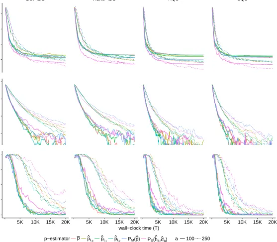
In the last part of this thesis, we present extensive numerical experiments in order to evaluate our sampling strategies (information-based or randomized). In particular we demonstrate the efficiency of randomized quantile sampling for balancing the ex-ploration/exploitation component; moreover, we show that spatial surrogate modeling results in significant gains relative to the local estimators, as quantified by the improved quality of the resulting root estimates (namely lower absolute residuals, narrower credible intervals and dramatically higher probability coverage). Our work is motivated by the root-finding sub-routine in pricing of Bermudan financial derivatives, illustrated in the last section of this thesis.

(11)

List of Figures

1.1 Knowledge updating for PBA. . . 8

2.1 Expected posterior pdf for p(·) given majority proportion. . . 28

2.2 Bias in knowledge states using local estimators forp(·). . . 30

2.3 Example of true and approximated knowledge states. . . 31

2.4 Data acquisition using the batched information criterion. . . 39

4.1 Graph of the three test functions used for numeric examples. . . 59

4.2 Average performance statistics for the linear function h1. . . 64

4.3 Comparison of surrogate models and sampling policies using Spatial G-PBA. 71 4.4 Adaptive replication scheme using Binomial Gaussian Processes. . . 73

4.5 Empirical analysis of the adaptive replication scheme using two different thresholding sequences and applied to the linear test functionh1. . . 76

4.6 Comparison of spatial sampling policies with respect to baseline policies. 79 4.7 Empirical distribution stochastic simulator for pricing a Bermudan finan-cial derivative. . . 81

4.8 Empirical distribution of root estimates using regression surface modeling approach. . . 83

(12)

List of Tables

2.1 Knowledge updating regimes using local G-PBA. . . 33 2.2 Average hitting time for the Test of Power One strategy using the test

functionh1. . . 34

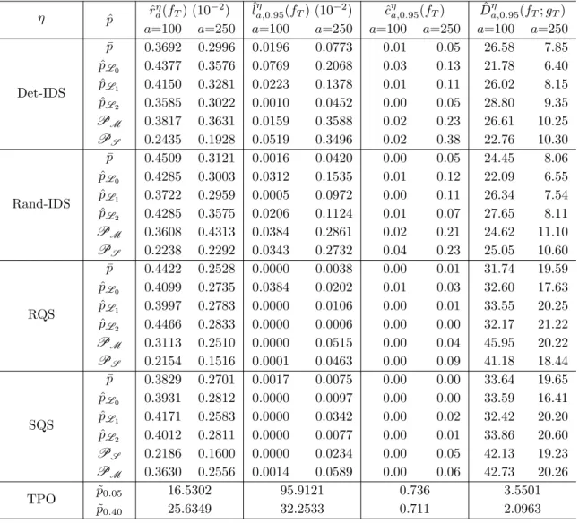
4.1 Performance metrics for the linear function h1 using the Local G-PBA. . 66

4.2 Performance metrics for the exponential functionh2 using the local G-PBA. 67

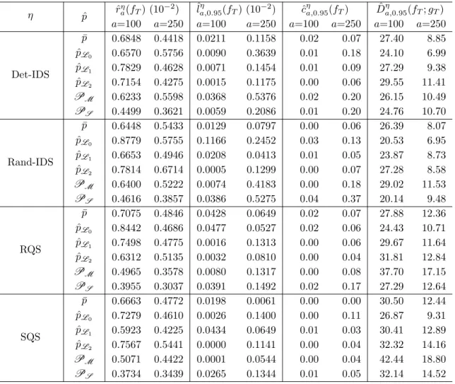
4.3 Performance metrics for the cubic function h3 using the Local G-PBA. . 68

4.4 Performance metrics for the linear test function h1 implementing the

spa-tial G-PBA. . . 74 4.5 Performance metrics for the exponential test functionh2implementing the

Spatial G-PBA. . . 77 4.6 Performance metrics for the cubic test function h2 implementing the

spa-tial G-PBA. . . 77 4.7 Performance metrics for the Optional Stopping Problem example using

(13)

Chapter 1 Introduction

1.1 Motivation

This thesis studies the problem of estimating the root of a function when the function is expressed implicitly through a stochastic simulation known as stochastic root-finding

problem (SRFP).

Our interest in studying SRFPs is motivated by the root-finding sub-routine for pric-ing a Bermudan Put option [39]. Namely, a stochastic simulation approach (known in the literature as the Longstaff-Schwartz paradigm [38]) recursively builds noisy simula-tions of the timing-value function; defined as the difference between the value function and the reward function for any given initial price x and fixed time t ≥ 0 [6]. This is obtained by generating forward paths of the state process and computing corresponding path-wise random reward. The realization,Z(x), is the path-wise timing valueh(x), that is, the difference between future and immediate reward over the given trajectory, which is furthermoreunbiased for the trueh(x). It is well-known that there is a unique exercise boundary, sayx∗, so that the timing-value is zero, i.e., h(x∗) = 0 and one should exercise as soon asxdrops belowx∗, since the conditional expectation of tomorrow’s reward-to-go

(16)

Section 1.1 Motivation is less than the immediate reward (frequently, a priori structure implies that thestopping set (0, x∗) is a half-line, i.e., h(·) has a unique root x∗). However, since the timing-value function h(·) is learned with noise that arises intrinsically due to the randomness in the simulation, finding x∗ effectively reduces to a SRFP.

Stochastic root-finding indeed ubiquitously in a wide range of applications. Some relevant applications of SRFPs include, for instance, the quantile estimation problem in Bio-assay experiments [18]; quality and reliability improvement [33]; sensitivity experi-ments [41]; and adaptive control and signal processing [12, 24, 5].

Data generating mechanism and experimental design. Throughout this thesis we work with ablack-box view of a simulation model, where the inputs and outputs of a simulation model are observed, but the internal variables and specific functions implied by the simulation are not. In particular, we assume a data generating process of the form

Z(x) =h(x) +(x), x∈(0,1); (1.1)

whereZ(x) is the simulation output,h(x) is a real-valued function and(x) is an additive noise component whose distribution depends upon the sampling location x (simulation input) but it is independent of previous evaluations. In addition, we assume that the search space is bounded, so we can scale the search region to be the interval (0,1).

We remark that the nature of the data generating mechanism (1.1) differs from the classical regression/machine-learning paradigm, where it is assumed that a data set (xi, Zi(xi))Ni=1 is available before inference about unknown parameters is performed. In

general, we are interested in settings where simulation evaluation is expensive and data collection is restricted to a limited a sampling budget N and hence experimental design (ED) becomes critical.

The goal of ED is to efficiently learn the root x∗ of the function h, interpreted as optimizing the simulation budget of calling (1.1) by judiciously selecting the pointsx1:n:=

(17)

Section 1.1 Motivation (x1, . . . , xn) at which to observe Z1:n := (Z1(x1), . . . , Zn(xn)), and in turn construct an

estimator ˆxn whose performance1 improves as more information is available. The latter

problem falls under the rubric of Bayesian design of experiments [11], in general; and design and analysis of simulation experiments (DASE) [36], in particular. Importantly, notice the distinction between sampling locations xn and the estimators ˆxn, which in

general need not to be the same (in contrast to deterministic root-finding algorithms where xn coincides with the estimated root ˆxn).

Roughly speaking, there exist two approaches to conduct an experiment, a sequential (adaptive) design or a passive (non-adaptive) design. In a passive design the querying locations x1:n are chosen prior to the experiment, whereas in a sequential design new

sampling points xn+1 are selected based on the previous x1:n and Z1:n. As pointed out

in [32], the optimal election of, xn+1, depends intimately on the distributional properties

of the simulation outputs Z(·) and, naturally, no information is available before the actual experiment is conducted. Thus, the root estimates induced by a passive design (e.g., sampling uniformly over the input space) may exhibit poor optimality properties, whereas a sequential approach may be a more suitable choice to learn the root. In fact, as we show in our numeric examples presented in Chapter 4, sequential strategies outperform their non-adaptive counterpart as measured by their corresponding accuracy and uncertainty reduction about the root location.

The primary focus of the work presented below is thus to develop statistical procedures to infer the point x∗ that solves h(x∗) = 0, by efficiently selecting the locations x1:n

at which to observe simulation outputs Z1:n and in turn produce a high-fidelity point

estimator ˆxn for the unknown root location x∗. To that end, we assume the existence

and uniqueness of the root x∗ on (0,1) so, without loss of generality, we furthermore

1_{For example, in our numeric examples presented in Chapter 4 we use several performance metrics to}

(18)

Section 1.1 Motivation suppose that the function h(·) in the metamodel (1.1) is positive to the left of x∗ and negative for all x > x∗ (e.g., is non-increasing on (0,1)).

Overview of Stochastic Root-Finding Methods. Numeric schemes for solving SRFPs can be classified broadly into two main groups: stochastic approximation and sample-path methods [43].

The stochastic approximation (SA) algorithm was introduced in the seminal paper of Robbins and Monro [50]. The SA paradigm closely resembles the Newton-Raphson deterministic root-finding regime for non-linear root-finding: start at a initial point x1

close fromx∗ is known to be located (usually the region at which the underlying function his monotonic is known a priori), and then evaluate (1.1) selecting new points using the rule

xn+1 :=xn−bnZn,

for all n ∈ _N until convergence criteria are satisfied; where (bn)n≥1 is a deterministic

sequence of constants. The SA strategy is in fact fully asymptotically efficient, i.e., xn→x∗ in probability as n →+∞ under regularity conditions on the tunning sequence

(bn) [32].

As mentioned in Waeber [57], one of the main drawbacks of the SA-type methods is that they only provide a point estimate ˆxnforx∗ (which under the SA setting is equal to

the sampling locationxn) without specifying any further probabilistic guarantees on the

accuracy of this estimate, for example, a confidence interval for the truex∗, which is one of the main tools necessary to determine a stopping rule when sampling budget is small. Another approach that implements the actual functional evaluations (1.1) consists of sample-path (SP) schemes [25, 54]. As mentioned in [43], the SP method is conceptually very simple and intuitive: substitute the unknown function h in (1.1) by a determin-istic function obtained by observing “realizations” of an unbiased estimator Zm for h

(19)

Section 1.1 Motivation (for example, the average function evaluations ¯Zm(·) := m−1Pm_j₌₁Zj(·)), and then solve

the resulting problem as a deterministic root-finding problem (DRFP). In this sense, a practical and viable strategy is thus to learn h(·) directly by regressing the batched re-sponses ¯Z1:n := ( ¯Zm(x1), . . . ,Z¯m(xn)) on the history of sampling locations x1:n, i.e., build

a surrogate ˆh and then take ˆx = ˆh−1_{(0) to be the root of ˆ}_h(_·_{), obtained via a standard}

deterministic root-finding method (say Newton’s method if ˆh0 is also available). In these scenarios, the practitioner is actually faced with an SRFP, but chooses, albeit implic-itly, to solve it as a DRFP. Surrogate modeling offers an opportunity to import the vast machinery of emulation/meta-modeling construction which is an extensive topic in the design of simulation experiments [36], as well as in the simulation optimization and computer experiment literatures [9]. Within this context, root-finding is equivalent to contour-estimation, i.e., learning the boundary of{x:h(x)>0}, see [47, 4, 23].

Some of the drawbacks of response surface modeling (RSM) described above is that a “good” representation for h usually does not lead to tractable models for ˆx. For example, consider a Gaussian process (GP) prior for h. A GP is a collection of random variables, any finite number of which have a joint Gaussian distribution [48]. Then, the marginal distribution h∗(x) is also Gaussian for any fixed x, however there is no

closed-form expression for the distribution of h−1

∗ (0). A viable choice to overcome the latter

limitation is for example build a bootstrapped empirical density for the root location based on iteratively estimating the root location as more data is available. Nevertheless, the latter heuristic ignores the dependency on the surrogate election as well as on the numeric error due to replacing the original problem of estimating the root x∗ with the RSM approach as we show in our numeric examples presented in Chapter 4.

The above limitation points to the second alternative of modelingx∗ itself, with has a background latent object. In this framework, statistical inference is conducted directly on the root, considering x∗ as an unknown parameter to be inferred via the realized

(20)

Section 1.2 Probabilistic Bisection for Stochastic Root-Finding data Z1:n obtained after sampling (1.1) at n locations x1:n. A natural strategy towards

constructing an estimator ˆxn for x∗ given Z1:n, is to follow a fully Bayesian approach:

update knowledge aboutx∗ based onprior information about the shape of the underlying functionh (e.g., h is non-increasing) and the evidence provided by the responses Z1:n —

whose statistical properties are governed by the distribution of the random component (·) in (1.1).

1.2 Probabilistic Bisection for Stochastic Root-Finding

One promising Bayesian alternative which accounts for both theestimationanddesign component is the Probabilistic Bisection Algorithm (PBA), recently applied to solve one-dimensional SRFPs by Waeber et al [57].

The PBA leverages the classical bisection search in a noise-free setting: iteratively halve the search region and then select a subinterval in which a root must lie for further processing. In the stochastic case, however, the PBA accounts for noise in the oracle responses by consideringx∗as the realization of an absolutely continuous random variable X∗ ∼ g0 with prior density g0 supported on (0,1). The PBA then works with the sign

of the noisy function evaluations,

Y(xn) := sign{Z(xn)}; (1.2)

which provide information as to whetherx∗ lies to the left or to the right of a given point xn, in order to subsequently update a posterior density for X∗,

gn(X∗) :=p(X∗|Y1:n, x1:n), (1.3)

that is, the conditional pdf of the root location X∗ given the history of oracle responses Y1:n := (Y1(x1), . . . , Yn(xn)), sampling locationsx1:n and prior g0.

(21)

Section 1.2 Probabilistic Bisection for Stochastic Root-Finding The posterior (1.3) then serves the twin purposes of guiding the election of the next sampling locationxn+1 at which to query (1.2), as well as to provide an estimator ˆxn for

X∗ (e.g., the posterior median or mean of gn).

Notice that due to the noise term (xn) in the simulation outputs Z(xn), then the

responses Y(xn) := sign{Z(xn)} translate into potentially inaccurate oracle directions.

To account for noise in (1.2) the PBA considers the probability of correct sign,

p(xn;x∗) :=P(Y(xn) = sign{xn−x∗}), xn, x∗ ∈(0,1); (1.4)

(henceforth referred as oracle specificity or accuracy), which is then used to update knowledge about X∗ by re-weighting the current gn proportionally to p(xn)≡p(xn;x∗).

Figure 1.1 shows an example of a realization of the classical PBA updatinggn (i.e., when

p(xn) is known) captured at stages n = 0,1,10, implementing a linear function,

h1(x) = x∗−x, x∈(0,1),

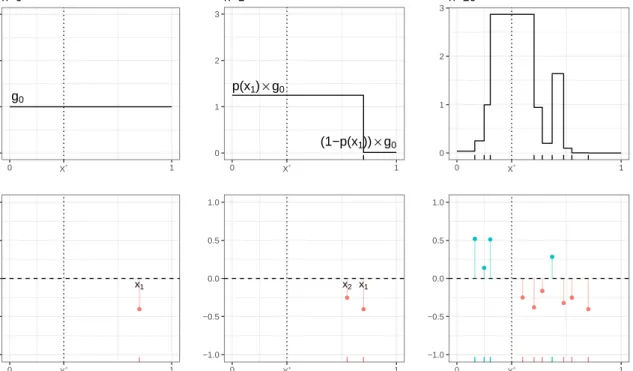
which is henceforth our running example with root at x∗ = 1/3. Figure 1.1 illustrates three fundamental components of the PBA:

• At each step the value ofp(·) is required to update fromgn togn+1. The top panel

of the second column in Figure 1.1 shows that the updating takes the prior g0

and then “re-calibrates” knowledge based on whether a positive/negative response Y(x1) is observed and the corresponding probability p(x1) of that direction being

correct after updating at x1.

• The PBA is able to account for noise in oracle directions Y(·) by assigning non-zero probability gn(·) at regions where X∗ is believed to be based on the history

of responses Y1:n. For instance, notice that after n = 10 most of the mass of gn is

(22)

Section 1.2 Probabilistic Bisection for Stochastic Root-Finding

• If one were to blindly apply deterministic bisection search for the stochastic case; a single wrong direction will divert the search path almost surely, as it is the case in the positive response observed rightwards x∗ as seen on the bottom right panel of Figure 1.1. g0 0 1 2 3 0 X∗ 1 P oster ior density n=0 ● x1 −1.0 −0.5 0.0 0.5 1.0 0 X∗ 1 Noisy sim ulation outputs p(x1)×g0 (1−p(x1))×g0 0 1 2 3 0 X∗ 1 n=1 ● ● x1 x2 −1.0 −0.5 0.0 0.5 1.0 0 X∗ 1 0 1 2 3 0 X∗ 1 n=10 ● ● ● ● ● ● ● ● ● ● −1.0 −0.5 0.0 0.5 1.0 0 X∗ 1

Figure 1.1: Knowledge updating using PBA with known p(x) at stagesn ∈ {0,1,10} using the linear test functionh1(x) :=x∗−xwithx∗= 1/3.

Classical PBA with constant and known oracle properties. Under the as-sumption that the oracle accuracy is known and constant (i.e., p(xn)≡p,∀xn), Waeber

at al. established exponential convergence of the posteriorgn to a Dirac mass at the true

x∗ when the next location is given by xn+1 = median(gn). While, in practice, these

con-ditions are not typically going to be satisfied (as in our Bermudan Put example outlined in Section 1.1), such explicit performance guarantees are highly desirable and have not been available via RSM approaches.

(23)

Section 1.3 Generalized PBA for Stochastic Root-Finding In a realistic context, the oracle specificity (1.4) is unknown and spatially varying in xn (since it intrinsically depends on h(xn) as well as on the statistical properties of

(xn) in (1.1)). Without further assumptions, the only way to employ PBA is toestimate

p(xn). This was already noted in [57, 19] where a hypothesis-testing-inspired procedure

was used to learn p(xn) en route to learning X∗. Specifically, they employed a Test of

Power One (TPO) [55], which relies on repeated sampling of (1.2) to effectively boost p(xn) to a fixed accuracy level ˜p(xn). However, such boosting can be very expensive in

the regime where p(xn) = 0.5 +δ for small δ > 0. This highlights the second challenge

with PBA: in the context of root-finding and (1.1), forxn close tox∗ we havep(xn)'0.5

which implies that the oracle isuninformative in the neighborhood of the root. A na¨ıve implementation of PBA leads to sampling too close to x∗ and is not asymptotically convergent in the sense of the posterior collapsing to a Dirac mass at x∗.

1.3 Generalized PBA for Stochastic Root-Finding

In this thesis, we resolve the inherent challenges in the classical probabilistic bisection scheme by providing a practically-minded extension of PBA. We construct a class of algorithms, which we term generalized PBA (G-PBA) that can:

(P1) efficiently learn oracle properties;

(P2) aggregate collected information to construct a sequential design; and

(P3) update knowledge about the root location as new information becomes available. To do so, similar to [57] we rely onbatched sampling to learnp(·); however in contrast to the latter TPO strategy that evaluates the oracle a random amount of times in order to avoid estimatingp(·) explicitly, we work with afixed batch sizea≥1. We demonstrate through the numeric examples presented in Chapter 4, fixed batching is more efficient,

(24)

Section 1.3 Generalized PBA for Stochastic Root-Finding in particular by providing better control over the size of each batch, as well as allowing the user to control the number of design points to be explored.

Estimating oracle properties. For (P1) we propose a collection of inference methods which leverage the fundamental assumption of the PBA for SRFPs, that the distribution of the noise component (·) is symmetrical. The latter allows for the re-parametrization of p(x) as:

p(x) = max{θ(x),1−θ(x)}, ∀x∈(0,1); (1.5) where

θ(x) := _P(Y(x) = +1) (1.6)

is the probability of observing a single positive response at x. Consequently, we will translate our inference problem of learning (1.5) into learning (1.6), to finally obtain plug-in estimators of the form

ˆ

p(x) = max{θ(x),ˆ 1−θ(x)ˆ }

for p(x). Naturally, the information that is used to find ˆθ(x) is B(x) :=

a X j=1

1{Yj(x)=+1}, (1.7)

which counts the number of positive responses observed at x after evaluating (1.2) a-times.

In this thesis, we present two inference paradigms which intrinsically are built upon the binomial response (1.7) and whose differences reside in whether spatial correlation across sampling locations and corresponding binomial responses is leveraged or not.

The first class of estimators which do not borrow information across sampling loca-tions is presented in Chapter 2, henceforth also referred aslocal estimators. An example of such estimators is the majority proportion estimator

¯

(25)

Section 1.3 Generalized PBA for Stochastic Root-Finding where θ(x) is estimated via the binomial proportion ¯B(x) := B(x)/a.

A key characteristic of the estimator ¯p(x) is the majority-vote property, that is, if a positive sign is observed majoritively at x (i.e., B(x) > da/2e), then the probability of an accurate oracle response p(x) >1/2 with high confidence. In Chapter 2 we analyze the statistical properties of ¯p(x) such as bias and consistency.

Within the same class of local estimators, we furthermore introduce a Bayesian fam-ily of statistical procedures, ˆp_L(x), based on a posterior density π(p|p(x)) for¯ p given the majority proportion ¯p(x) and a prior distribution for p ∼ π0. With π(p|p(x)) in¯

closed-form we propose a collection of optimal Bayes estimators based on several loss functions L.

In Chapter 3, we present a second estimation paradigm which is able to borrow information across sampling locations. To do so, we deploy spatial surrogate models which rely on a classical binomial (logistic) regression approach: it is assumed that the locations xi’s are related to θ(xi) via the canonical Bernoulli link function

log θ(xi) 1−θ(xi) =ϕ(xi), i= 1, . . . , n;

and where x 7→ ϕ(x) is a surrogate model to be trained from the data (xi, Bi(xi))ni=1

for n < N. Specifically, we seek non-parametric regression approaches which are able to refine the regression curve in regions where more data points are placed (namely close to the root), and simultaneously give a good global fit. In particular, we implement two families of surrogates:

(A) a Gaussian random field (GRF) modeling approach (also known as Gaussian process modeling, [48]) that takesϕas a latent Gaussian process and outputs the posterior distribution p(ϕ∗|Dn) conditional on the data Dn:= (B1:n, a1:n, x1:n); and

(26)

Section 1.3 Generalized PBA for Stochastic Root-Finding by a collection of basis functions, i.e., ϕ(x) = Pp

j=1βjφj(x), with the coefficients

β:= (β1, . . . , βp).

Both modeling schemes (A) and (B) are mathematical approximations (metamodels) capable of modeling the relation x 7→ θ(x). Metamodels are particularly useful since they can be built upon available observations and updated when new data is assimilated. They can also be used to guide simulator evaluations more efficiently [51]. Given the fitted surrogate ˆϕn, the estimate for p(·) is a plug-in estimate of the form:

ˆ

pn(·) := max{θˆn(·),1−θˆn(·)}; where ˆθn(·) := [1 +e−ϕˆn(·)]−1. (1.8)

Binomial Gaussian Processes and Adaptive Querying. In the context of inferring θ(x)

a fundamental question is to optimally determine optimally the amount of replication a(x) at each locationxwhere the batched responseB(x) is observed. The answer to this question is primarily driven by two concepts: (i) accuracy, as measured by successfully predicting p(x) at values of x which are close from the root x∗; and (ii) allowing the algorithm to explore the search region in a way that maximize computational efficiency. The latter idea has been already posed for the problem of design of GP surrogates in the face of heteroscedastic simulation experiments. Namely, Binois et al. [8] study the conditions under which the new element should be a replicate versus explore a single response. Analogous to the latter approach, we utilize the Binomial GP surrogate (A) to adaptively determine the batch size an+1 as a function of the sampling location xn+1 in

order to address the replication/exploration trade-off (which becomes critical at locations close from the root location).

In this context, in Chapter 3 we present an approximated adaptive replication scheme wherean+1 is computed as a function of the estimated predictive variance atxn+1.

Intu-itively, this approach will employ a larger batch size at locations where the posterior un-certainty of the latent is large and a smaller batch size for locations whereθ(·) has already

(27)

Section 1.3 Generalized PBA for Stochastic Root-Finding been learned sufficiently well. We again contrast this adaptive replication regime with TPO, in which querying ignores previous information leading to oversampling, whereas in our approach the replication size can be as small as an+1 = 1 for locations where the

predictive variability ofθ(·) is sufficiently small.

Sampling policies. A sampling policy η is a rule which maps states to actions. In the context of SRFP actions effectively correspond to selecting sampling locations xn+1. As in standard PBA, we work in the sequential paradigm for (P2), selecting

xn+1 based on a Bayesian perspective. Namely, to generalize the ideas of PBA to the

setting of unknown p(·) we introduce a knowledge state. The state of a system can be described as consisting of all the information needed to make a decision, compute the objective (contributions and rewards), and compute the transition to the next state [45]. The knowledge (or belief) state fn captures our distribution of belief about X∗ that we

do not know perfectly. The underlying philosophy is a Bayesian formulation of SRFP, translating the task of learning the rootX∗ into the language of “beliefs” encapsulated by fnand used to quantify (posterior) uncertainty aboutX∗. Intuitively,fnis a “surrogate”

to the true posteriorgnthat is no longer attainable due to unknown p(·). The knowledge

state fn is then used for the dual purposes of providing an estimate ˆxn of X∗, and for

guiding the sequential design.

We propose a collection of sampling strategies which blend the estimation procedures ˆ

p developed for (P1) with the concept of information directed sampling and quantile-sampling strategies. We also show the effectiveness of randomization for both schemes which turns out to be crucial in preventing uncontrolled error propagation in constructing the knowledge state. In Chapter 2 and Chapter 3 we compare respectively the perfor-mance of such policies using local and spatial modeling for inferring p(·).

Knowledge Updating. The main challenge under the G-PBA paradigm where we have unknown and location-dependent oracle accuracy, is that estimation for p(·)

(28)

Section 1.3 Generalized PBA for Stochastic Root-Finding and knowledge updating about X∗ must be performedsimultaneously. Towards address-ing (P3), in Chapter 2 we explicitly construct an updataddress-ing mechanism

fn+a:= Ψ(fn, xn+1; ˆpn+1, an+1)

capable of blending both estimation and knowledge state updating about X∗.

To obtain theknowledge transition functionΨ(·) we extend the classical PBA Bayesian updating regime to construct a batched version which relies on sampling an+1

replica-tions at xn+1 and observing the total number of positive responses B(xn+1) in order to

construct ˆpn+1. Given an+1 and ˆpn+1 knowledge updating occurs necessarily from fn to

fn+a. This knowledge updating mechanism given by Ψ(·) represents some of the main

contributions of this thesis and are presented in Chapter 2.

1.3.1 Summary of Contributions and Related Literature

Our G-PBA schemes are generic in that they make minimal assumptions about the underlying (1.1), and can be employed across a wide spectrum of SRFP’s. To illustrate this robustness we use G-PBA on our motivating example above to learn the critical exercise threshold in the context of Regression Monte Carlo for Optimal Stopping. In that case, the behavior of (1.1) is highly non-standard, expressing strongly heteroskedastic and non-Gaussian characteristics, to which standard statistical learning procedures for ˆh are very sensitive [39]. In contrast, the G-PBA is rather agnostic with respect to the usual homoscedasticity and Gaussianity assumptions, not least thanks to the batching sub-steps which allow for the Central Limit Theorem (CLT) to smooth statistical anomalies. To provide further context for this thesis, let us recapitulate our contributions relative to existing methods. Our contributions can be traced along several directions.

First, compared to PBA, we work withunknown andlocation-dependent oracle accu-racyp(x), which requires a complete re-imagining of the algorithm, focusing on practical

(29)

Section 1.3 Generalized PBA for Stochastic Root-Finding solutions that work well in non-asymptotic settings, where we are constrained by the bud-get ofT available oracle calls. In particular, we contrast our strategies with the proposals in [57, 19] that employ the TPO approach to learn p(x), as we will show, while TPO enjoys nice theoretical properties and is a viable alternative in terms of its asymptotic behavior, it performs poorly for a small sampling budget T.

Second, compared to simulation optimization, we develop a root-finding procedure which is built around the notion of constructing an explicit posterior density for the root, and hence, primarily operates with the knowledge state rather than a surrogate forh(·). This allows us to obtain and monitor the (pseudo-) credible bands for X∗ which give sequential quantification of the learning performed by PBA. Thusly, we contribute to the greater stochastic root-finding toolkit.

Finally, our sequential updating and sampling strategies can be linked to the literature on active learning since they are based on the posterior uncertainty quantification of X∗ rather than an h-based statistic — grounding our method in a purely information-theoretic paradigm. In that sense, we make use of an acquisition function [11] which maps previously assimilated information that is condensed by the surrogate.

(30)

Chapter 2 Generalized Probabilistic Bisection

2.1 Introduction

A complete solution to the SRFP using the PBA was provided by [59] under the key assumption that the oracle specificity (1.4) is a known and x-independent constant, i.e., p(x) ≡ p,∀x ∈ (0,1) . Namely, Waeber et al. derived the equations for the posterior density

gn(X∗) := p(X∗|y1:n, x1:n) (2.1)

and then established that sampling at the posterior median, xn+1 := G−n1(0.5) for all

n = 1,2, . . ., is an optimal policy. More precisely, they proved that this sampling rule minimizes the expected Kullback-Leibler (KL) distance for its utility function, and most importantly achieves exponential convergence for the estimate ˆxn ≡ xn towards

x∗, i.e., |xˆn− x∗| = O(e−αn) with an explicit expression for α > 0. This justifies its

name, as the PBA manages to effectively reduce the interval containing x∗ by α% at each stage. This result is truly impressive both given the noisy oracle replies and thanks to the simplicity of the sampling rule. This assumption of spatial oracle stationarity would tend to be met in applications where the transition between regions inhis abrupt.

(31)

Section 2.1 Introduction As an example, if a city’s water supply were contaminated with a dangerous chemical we would want to localize the extent of contamination as quickly as possible, and if the chemical did not dissolve well in water but instead tended to stay concentrated, we would face a situation with such abrupt transition between contaminated and uncontaminated water [45]. Moreover, PBA exemplifies the Bayesian setup: xn+1 is selected based on the

information summarized by gn, which also yields the point estimate ˆxn.

Some partial results extending to the case wherep(x) is non-constant (but stillknown) were given in [58]. The crucial assumption that oracle properties, specifically p(x) is known, is hard to justify in the context of unknown response h(·). For example, when the noise component in (1.1) is (x) ∼ N(0, σ2_{(x)), then} _{p(x) = Φ (}_|_h(x)_|_{/σ(x)), where}

Φ(·) is the cumulative distribution function (CDF) of a standard Gaussian, and therefore knowledge of p(·) is equivalent to knowing the signal-to-noise ratio — a rather unlikely proposition. At the same time, the known-p assumption is critical to the performance: as we discuss below without further modifications the PBA might fail completely in the context of unknown p(x). More sophisticated sampling strategies are needed to resolve this tension between exploitation and exploration.

To generalize the ideas of PBA to the setting of (1.1) we introduce a knowledge state, fn, that is recursively updated and used for acquiring new samples. The underlying

phi-losophy is a Bayesian formulation of SRFP, translating the task of learning the root into the language of “beliefs” encapsulated byfnand used to quantify (posterior) uncertainty

about X∗. Intuitively, fn is a “surrogate” to the true posterior (2.1) that is no longer

attainable due to unknown p(·).

A key ingredient of our approach is the use of replications: repeatedly evaluating the oracle a ∈ _N times at a fixed sampling location x. In this sense, a is the “sample size” (akabatch size), that is, some measure of simulation effort that is usually well-defined de-pending on the context. In the context of terminating simulations, for example,ausually

(32)

Section 2.1 Introduction refers to the number of times the simulation is called in computing the estimator ˆp(x). In non-terminating simulations,a usually refers to the “length of time” the simulation is executed when computing the estimator ˆp(x) [43].

Replications (henceforth also referred as batched sampling) allows us to obtain a point estimate ˆp(x) for p(x) based on counting the total number of positive responses B(x) observed at xas in (1.7), which is then used to update knowledge from fn tofn+a.

Replicates decouple the problems of learningX∗ and of learningp(·); they also boost the signal-to-noise ratio which allows faster convergence at the macro-level. Our resulting G-PBA framework learns in parallel X∗ and p(·) and is summarized in Algorithm 1.

input :Total query budgetT; batch sizeaand prior distributionf0 on the root.

forn←0,1, . . . , N−1 do

Generate next sampling point xn+1;

Obtain the estimate ˆp(xn+1) using the binomial response B(xn+1);

Update knowledge state to fn+a:= Ψ (fn, xn+1, B(xn+1); ˆp(xn+1), a);

end

returnRoot estimate ˆxN; Knowledge statefT.

Algorithm 1: Generalized PBA. In order to implement Algorithm 1, the G-PBA must specify: (GPBA-I) statistical procedure ˆp(xn+1) for estimatingp(xn+1) at xn+1.

(GPBA-II) the mechanism to update knowledge states Ψ :fn→fn+1;

(GPBA-III) the rule η for selecting xn+1 =η(fn) givenfn;

All three of the steps (GPBA-I), (GPBA-II) and (GPBA-III) require novel analysis, and are a part of the main contributions of this thesis.

(GPBA-I) Statistical procedure for estimating p(·). All three steps above require knowledge of p(x), so proper inference of the latter is central to the G-PBA

(33)

Section 2.1 Introduction performance. The symmetrical noise distribution assumption in (1.1) implies that the oracle is “democratic”: p(x)≥0.5∀x, and thus there is an implicit majority-vote property inp(x), whereby the estimate is based on the majoritatively observed sign of the binomial response B(x). This introduces a fundamental bias which becomes especially significant when sampling close to X∗ (|h(x)| is small and p(x)'0.5).

In Section 2.2 we investigate three types ofp-estimators: frequentist based on majority proportion; Bayesian based on the posterior density of p given B(·); and a collection of boosted estimators which directly aggregate oracle responses to construct a subsidiary signal whose specificity is enhanced thanks to batching.

A fundamental property of the statistical procedures developed under this setting, is that p(x) is inferred based solely on the information collected at x via the summary statistic B(x). In this thesis, we refer to the latter paradigm as local estimation as no information across sampling locations in leveraged for constructing the estimator ˆp(x) at location x.

(GPBA-II) Knowledge Updating Procedure. To update fn we then plug-in

an estimated ˆp(x) into a knowledge state transition function of the form

fn+a := Ψ (fn, xn+1, B(xn+1); ˆp(xn+1), a), n= 0,1, . . . , N −1 and a∈N, (2.2)

where the sufficient statistic B(xn+1) is defined in (1.7). The map (2.2) is the analogue

of Bayesian updating whenp(x) is known . Note that the knowledge transition Ψ(·; ˆp, a) function is similarly batched, allowing us to make full use (while maintaining compu-tational efficiency) of the sampled replicates. This aspect is fully addressed in Section 2.2.

(GPBA-III) Sampling Policies. Third, to select the locations xn+1 at each

n = 0, . . . , N −1 we introduce several sequential sampling policies η. The first fam-ily of Information Directed Sampling uses an information gain function I(x, fn;p(x), a)

(34)

Section 2.1 Introduction to quantify the learning rate for X∗ if a new query batch is done atx. Notice that the acquisition function x 7→ I(x, fn;p(x), a) depends on either the knowledge statefn and

the nuisance parameter p(x) for each x for fixed batch size a. It is motivated by the optimality property of standard PBA in terms of maximizing the KL relative entropy between gn and gn+1.

The second family of Quantile Sampling is motivated by the other aspect of PBA, namely of sampling at the median of the knowledge state. Letting Fn be the CDF

of fn, we therefore propose to use the quantiles of fn for selecting the next xn+1, i.e.,

xn+1 :=Fn−1(q), where q ∈(0,1).

Another important computational adjustment that we entertain is an additional de-gree of randomization which serves to (a) alleviate the issue of error accumulation arising from uncertainty in estimating p(xn) and (b) enforce exploration of the state space in

order to accelerate convergence to the trueX∗. Our experiments demonstrate the value of such randomized sampling policies and can be viewed as analogues of similar stochastic searches in Bayesian optimization (such as Thompson sampling [53]). Full analysis of these designs is in Section 2.3.

Wall-clock and macro time. Note that due to batching G-PBA will have two different time scales: macro-iterationsn = 1, . . . , N corresponding to the query locations x1:n, where N is the total number of sampling points for a fixed batch size a; and

wall-clock time, T = a×N, which counts the total number of oracle queries and hence the overall computational expense.

Estimating the rootX∗. The final ingredient is the rule ˆxnto construct an estimate

of the root based on fn. In analogy to the classical PBA setting, in this thesis we utilize

(35)

Section 2.2 Knowledge States is often skewed or multi-modal),

ˆ

xn := median(fn). (2.3)

2.2 Knowledge States

Consider a real-valued continuous response functionh: (0,1) → _R. For concreteness we have re-scale the (bounded) input space to the unit interval. The functionh is noisily sampled via the stochastic simulator (1.1). Let X∗ be the random root location and x∗ its realized value at which h(x∗) = 0. To learn x∗, the PBA works with the signs Y(x) := signZ(x), which due to the stochastic nature of the responses (1.1), are correct with probability p(x).

Assuming that p(x) is known, the next Lemma provides the analytical one-step up-dating equations for the posterior gn of X∗ defined in (2.1).

Lemma 2.2.1 (Updating formula for posterior density of the root location X∗). [59] Let x∈(0,1), Gn be the CDF ofgn and p(x) as in (1.4). Define

γn(x;p(x)) :=p(x)[1−Gn(x)] + [1−p(x)]Gn(x), (2.4)

Given a priorg0 onX∗ we have the recursion:

gn+1(u) = 1 γn(x;p(x)) p(x)1{u≥x}+ (1−p(x))1{u<x} gn(u), (2.5a)

if a negative sign is observed at x, i.e.,Yn(x) = +1; and

gn+1(u) = 1 1−γn(x;p(x)) (1−p(x))1{u≥x}+p(x)1{u<x} gn(u), (2.5b)

otherwise, for all n = 0,1, . . ..

Remark 1. If no prior knowledge about the root location X∗ is provided, then a sensible choice is a vague priorg0 =Unif(0,1). The latter is also computationally convenient, since

(36)

Section 2.2 Knowledge States (2.5) then implies thatgn will be piecewise constant ∀n, with discontinuities precisely at

the sampled x1:n. Therefore, storage and updating of gn becomes an O(n) operation in

this setup.

2.2.1 Batched Querying

Abstractly, the updating (2.5) constitutes a knowledge transition function Ψ : gn 7→

gn+1, which takes as inputs the current knowledge state gn, the oracle response Yn(x)

and its specificity p(x) when queried at the point x ∈ (0,1). To learn p(x), we employ batched queries, keeping the sampling locationxunchanged for a≥2 steps. Considering the resulting i.i.d. sequence of oracle responses (Yj(x))aj=1, the knowledge stategncan be

recursively computed by using the update (2.5) a-times to obtain gn+a. Because p(x) is

the same across those updates, we can simply consider the total number ofpositive oracle responses observed atx,B(x), yielding an aggregated knowledge transition function from gn togn+a.

Remark 2. The summary statistic B(x) defined in (1.7) intrinsically depends on the

sampling location x, as well as on the batch size a. However, in order to ease our notation we omit the dependency of B(x) on a, unless necessary.

Theorem 2.2.2 (Batched Bayesian knowledge transition function). Letgn be the current

knowledge state about X∗ and p(·) the probability of a correct oracle response. The batched Bayesian updating, Ψ, which maps gn to gn+a := Ψ(gn(u), x, B(x);p(x), a) is

given by gn+a(u) =      c−_n1(x)p(x)B(x)(1−p(x))a−B(x)·gn(u) if 0< x < u <1, c−1 n (x) (1−p(x))B(x)_p(x)a−B(x) ·gn(u) if 0< u≤x <1; (2.6)

for all x∈(0,1) with normalizing constant cn(x) :=

(1−p(x))B(x)p(x)a−B(x)Gn(x) +

(37)

Section 2.2 Knowledge States

Proof. We will show that the updating equations (2.6) hold for any a ∈ _N via

mathe-matical induction. To do so, letx be a fixed sampling location in the support ofgn, and

B ∈ {0,1, . . . , a} to be the total number of observed positive signs after querying the oracle a ≥ 1 times at x, and Yj ∈ {−1,+1} the j-th oracle response observed at x for

j = 1, . . . , a(dropping the dependency onx and ainB and the Yj’s). Re-expressing the

knowledge transition function (2.6) using indicator functions as (and disregarding the normalizing constantcn(x) in (2.7)): gn+a(u)∝ " _a X j=0 pj(1−p)a−j1{B=j} # gn(u)1{u≥x}+ " _a X j=0 (1−p)jpa−j1{B=j} # gn(u)1{u<x},

with p ≡ p(x), we will prove that (2.6) holds for any a and fixed n. For a = 1 we have

{B = 1}={Y1 = +1}and {B = 0} ={Y1 =−1}and (2.6) corresponds to the updating

in (2.5). We now concentrate on the case u > xand inductively suppose Equation (2.6) holds for a; we now establish it for a+ 1:

gn+(a+1)(u)∝ (1−p)1{Ya+1=−1}+p·1{Ya+1=+1} gn+a(u) =(1−p)1{Ya+1=−1}+p·1{Ya+1=+1} × " _a X j=0 pj(1−p)a−j1{B=j} # gn(u) =: (A1+A2)gn(u). We now have A1 = a X j0₌₀ pj0+1(1−p)a−j01{B=j0_,Y a+1=+1} = a+1 X j=0 pj(1−p)a+1−j1{B=j−1,Ya+1=+1}.

Similarly we obtain A2 =Pa_j₌₀+1pj(1−p)(a+1)−j1{B=j,Ya+1=−1}, which implies that

A1+A2 = a+1 X j=0 pj(1−p)(a+1)−jh1{B=j,Ya+1=−1}+ 1{B=j−1,Ya+1=+1} i = a+1 X j=0 pi(1−p)(a+1)−j1{Ba+1=j}.

(38)

Section 2.2 Knowledge States Hence, if we furthermore define the right scaling-factor

ρ(x, B(x);p(x), a) :=p(x)B(x)(1−p(x))a−B(x), (2.8)

then the ratio

R(a)(gn, x, B(x);p(x)) :=ρ(x, B(x);p(x), a)/cn(x) (2.9)

completely specifies Ψ in (2.6): given the total number of positive responses B(x) ∈ {0,1, . . . , a}, the new posterior gn+a(u) is recovered by scaling the values of gn(u) for

x ≤ u by the factor ρ from (2.8) divided by the normalizing constant cn(x) from (2.7).

Hence, if B(x)>ba/2c, i.e., there is favorable evidence that x∗ is rightwards of x, then the mass of gn+a is shifted to the right of x. In the case where p(x) ∈ {0,1}, (2.8) is

defined by ρ(x, B(x);a, p(x)) := p(x), which effectively reduces the support of gn+a by

placing zero mass on one of the intervals that have x as an end-point.

Approximate Knowledge State fn. For our G-PBA algorithms, neither (2.5)

nor (2.6) are feasible, since they require the unknown p(x). Nevertheless, to mimic the Bayesian updating paradigm we introduce an approximate knowledge state fn which

follows the transition function in (2.6) by plugging-in an appropriate estimate ˆp(x), i.e., fn+a := Ψ(fn, x, B(x); ˆp(x), a); a≥2 and x∈(0,1), (2.10)

for n= 0, . . . , N −1 and where Ψ(·; ˆp, a) is computed via Theorem 2.2.2, for fixeda and statistical procedure ˆp. Note that because (2.10) is necessarily an approximation,fndoes

not match the true posteriorgn.

2.2.2 Frequentist and Bayesian Estimators for

p

(

· )

The task in this section is to perform statistical inference on the unknown (nuisance) parameterp(x) required to implement Bayesian updating aboutX∗, by using the batched i.i.d. responses (Yj(x))aj=1 observed at x ∈(0,1). As mentioned above, we thus leverage

(39)

Section 2.2 Knowledge States the symmetry of the noise component in the underlying noise component (1.1) so p(x) is re-parametrized via

p(x) = max{θ(x),1−θ(x)}; where θ(x) :=_P(Y(x) = +1) (2.11) is the marginal probability of observing a positive sign at location x. For the remainder of the section we consider a single (macro)-iteration of the overall G-PBA, treating the sampling locationxas fixed and suppressed from the notation. To estimatepwe construct an estimator forθ and then plug into (2.11).

From a frequentist perspective, we recall that the binomial proportion B/a is an UMVUE for θ and B ∼ Bin(a, θ) [10]. This yields the majority proportion estimator ¯p obtained by replacing θ by B/a in (2.11):

¯

p≡p(B) := max¯ {B/a,1−B/a}. (2.12) In Lemma 2.2.3, we show that _Ep[¯p]> p is necessarily biased high as soon asp > 1/2.

Lemma 2.2.3 (Bias of Majority proportion estimator ¯p). We have that the bias of of the majority proportion estimator ¯p given pis

Biasp(¯p) := EBp[¯p−p] =Pθ(B ≤ da/2e −1)−2pPθ(Ba−1 ≤ da/2e −2)>0, a≥3 (2.13)

Proof. For brevity, we drop the dependency on x.

EBp[¯p(B)] :=E B

p[max{B/a,1−B/a}]

= 1 a EBθ[B1{B≥da/2e}] +EBθ[(a−B)1{B<da/2e}] = 1 a EBθ[B] +aPθ[B <da/2e]−2EBθ[B1{B<da/2e}] =p+_Pθ(B <da/2e)− 2 aE B θ B1{B<da/2e} . (2.14)

The last term is equal to

Eθ h B1{B<da/2e} i = da/2e−1 X i=1 i a i pi(1−p)a−i (2.15)

(40)

Section 2.2 Knowledge States =ap da/2e−1 X i=1 a−1 i−1 pi−1(1−p)(a−1)−(i−1) =ap_Pθ(Ba−1 ≤ da/2e −2), Ba−1 ∼Bin(a−1, θ).

Substituting the latter quantity into (2.14) and usingBiasp(¯p(B)) :=p−Eθ[¯p(B)] yields

(2.13).

Intuitively, the bias in (2.12) is due to the possibility that the majority vote points in the wrong direction.

An alternative estimation procedure is to assign a prior for p and then construct a posterior based on the evidence (likelihood) provided by the batched responses ¯p. Using (2.12) yields the respective conditional likelihood of ¯pas:

Lemma 2.2.4 (Likelihood function of majority proportion). Let x be a fixed sampling location at which the oracle is queried a ≥ 2 times and B be the total number of positive responses observed atx. Then, the likelihood function of the majority proportion estimator, ¯p(B) := max{B/a,1−B/a}, in p is given by

Pp(¯p(B) =j/a) =     

Bin(j;a, p) +Bin(j;a,1−p), j = 0,1, . . . ,(da/2e −1); Bin(a/2;a, p), j =da/2e;

(2.16)

where dae is the ceiling function, and Bin(j;a, θ) is the probability mass function (pmf) of a binomial random variable in a ≥ 1 independent trials and success probability θ evaluated at j = 0, . . . ,da/2e.

Proof. GivenB ∼Bin(a, θ(x)) andθ(x) := _P(Y(x) = +1) = p(x)1{x∗_≤_x_}+(1−p(x))1_{_x∗_>x_}

for x∈(0,1), we have

Pp(¯p(B) = j/a) :=Pp(max{B/a,1−B/a}=j/a)

(41)

Section 2.2 Knowledge States = a j θj(1−θ)a−j+ a a−j θa−j(1−θ)j, ∀j = 0,1, . . . ,da/2e −1;

which is the sum of two binomial densities. Finally, if j = a/2 then _Pp(¯p(B) = 1/2) = Pθ(B =a/2) which is a single binomial density.

Assuming a vague prior p ∼ Unif(1/2,1) (recall that by construction p is known to be p≥1/2) we then obtain explicitly the posterior density π(p|p).¯

Theorem 2.2.5 (Posterior density of p given majority proportion ¯p). Suppose that p has prior densityπ0(p) = 2·1{p∈[1/2,1]}. Then, fora≥2, the posterior density ofpconditioning

on the majority proportion (2.11) is given by

π(p|j/a)∝      pj(1−p)a−j+ (1−p)jpa−j, if j = 0,1, . . . ,(da/2e −1); pa/2₍₁₋_p)a/2_, _if _j ₌_d_a/2_e_. (2.17) Proof. π(p|p(B) =¯ j/a)∝_Pp(B =j)π0(p) ∝ a j [pj(1−p)a−j + (1−p)jpa−j]1(1/2,1)(p), if j = 0,1, . . . ,(da/2e −1);

with the normalizing constant β1 =

R1

1/2[p

j₍₁₋_p)a−j_{+ (1}₋_p)j_pa−j_]_dp _{which can be}

expressed in terms of the Beta function.

Remark 3. Other priors (e.g. location-dependent) for pcan be entertained. TheUniform choice is convenient both as a vague prior, and due to it matching the conjugate Beta-binomial updates.

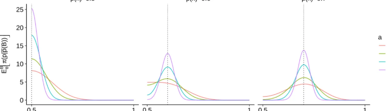
Figure 2.1 shows the theoretical expected posterior density, ˆπ(p;x, a) :=_EB

θ[π(p|p(B))],¯

obtained after averaging the posterior (2.17) with respect toB(x)∼Bin(a, θ(x)) for batch size values a ∈ {50,100,250,500} and locations x > x∗ so that p(x) ∈ {0.5,0.60,0.70}, implementing the test function h1(x) = x∗ −x presented in Section 4.1 which

(42)

Section 2.2 Knowledge States namely shows that posterior is unimodal around the true p(x); furthermore the posterior predictably tightens as a increases locating most of the posterior mass around the true p(x)-value. p(x)=0.5 p(x)=0.6 p(x)=0.7 0.5 1 0.5 1 0.5 1 0 5 10 15 20 25 p Eθ B π (p| p (B ))   a 50 100 250 500

Figure 2.1: Expected posterior pdf ˆπ(p;x) obtained with respect to B(x)∼Bin(a, θ(x)) for locationsx

so thatp(x)∈ {0.50,0.60,0.70} (columns) and batch sizea∈ {50,100,250,500}(lines).

Withπ(·|p(B)) in closed-form, we can obtain a variety of estimators ˆ¯ p_L(¯p) by mini-mizing the Bayesian posterior expected loss for a given loss function L(p,p). Namely,ˆ

(i) posterior mode based on L0(p,p) := 1ˆ {|pˆ−p|>,>0} (taking ↓ 0 as π(p|·) is

uni-modal),

ˆ

p_L₀(¯p) = modeπ(p|p);¯ (2.18)

(ii) posterior median based on the L1 lossL1(p,p) :=ˆ |p−pˆ|:

ˆ

p_L1(¯p) = medianπ(p|p),¯ (2.19)

(iii) and posterior mean based on the L2 lossL2(p,p) := (pˆ −p)ˆ2:

ˆ

p_L2(¯p) = mean π(p|p)¯ (2.20)

Remark 4. Practically, (2.18) and (2.19) have to be computed numerically, whereas (2.20) is computed in closed form as stated in Corollary 2.2.6.

(43)

Section 2.2 Knowledge States Corollary 2.2.6. The posterior mean ˆp_L₂(j/a) :=_Ep_B[p|p(B) =¯ j/a] is computed consid-ering two cases:

(i) If j = 0,1, . . . ,(da/2e −1)/a, then

ˆ p_L₂(j/a) :=β₁−1 ( B(j+ 2, a−j + 1)(1− Z 1/2 0 Beta(p;j+ 2, a−j + 1))dp +B(a−j+ 2, j + 1)(1− Z 1/2 0 Beta(p; (a−j+ 2, j + 1)dp ) .

(ii) If j =a/2, then

ˆ

p_L₂(j/a) =

n

B(a/2 + 2, a/2 + 1)(1−R1/2

0 Beta(p;a/2 + 2, a/2 + 1))dp

o

B(a/2 + 1, a/2 + 1)[1−R1/2

0 Beta(p;a/2 + 1, a/2 + 1)dp]

;

where B(a, b) := R₀1ua−1₍₁₋ _u)b−1_du _{is the Beta function defined for} _{a, b >} _{0; and}

Beta(u;a, b) is the pdf of a Beta random variable evaluated at u∈(0,1).

Remark 5. The above Bayes estimators depend on four different parameters: the

sam-pling location x, realized number of positive responses atxsummarized via the majority proportion ¯p(B(x)); the batch size a and the loss function L. Whenever necessary we denote such dependency explicitly by ˆp_L(¯p(B(x))).

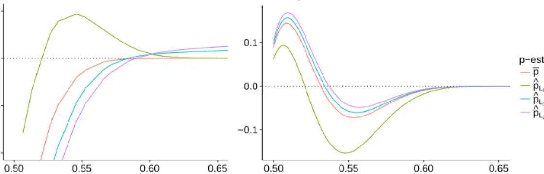
The left panel of Figure 2.2 shows the theoretical expected bias Biasp(ˆp(x)) := EBθ,x[p(x)−p(B(x))] corresponding to the estimators (2.12), (2.18), (2.19) and (2.20);ˆ

for a = 250 and p ∈ (0.5,1). Note that as p ↓ 0.5, all procedures overestimate the true p, highlighting the difficulty to estimate p(x) when x ' x∗. Of course, this issue is mitigated as batch size a increases. The procedures which best approximate p when p'1/2 are the posterior mode, ˆp_L₀, and the empirical majority proportion ¯p. However, as the true p increases, ˆp_L0 underestimates p (the bias increases), whereas the bias in

the empirical majority proportion decays uniformly. Conversely, both the posterior mean ˆ

(44)

Section 2.2 Knowledge States −0.010 −0.005 0.000 0.005 0.50 0.55 0.60 0.65 p(x) Actual − Estimated

Point Estimation Bias

−0.1 0.0 0.1

0.50 0.55 0.60 0.65

p(x) Scaling factor bias

p−estimator p p^L0

p^L1

p^L2

Figure 2.2: Left: Expected bias of ˆp-estimators with respect to the number of positive responsesB ∼

Bin(a, θ). Right: Expected right scaling factor ˆR(a)(f0, x,pˆ) computed givenf0=Unif(0,1) and several

locationsx > x∗ _{so that}_p₍_x₎_∈₍₀_.₅₀_,₀_._{70) (}_x_{-axis). Both panels are for}_a_{= 250.}

2.2.3 Bias in Knowledge States

Recall that the key component about the update fn+a (obtained via the

knowl-edge transition function Ψ) is given by the right-scaling factor (2.9) since it condenses all information needed in order to recover fn+a given fn. The average scaling

fac-tor integrated against the pmf of B is ˆR(a)_(f

0, x; ˆp) := EBθ,x[R(a)(f0, x;B,p(B))], whereˆ

B(x)∼Bin(a, θ(x)). The right panel of Figure 2.2 shows the expected right-scaling factor obtained given a Uniform prior f0 over (0,1) and updating locations x1 > x∗ labeled via

theirp(x1) (x-axis). Sincex1 > x∗, the right-scaling factor is expected to be close to zero

when p(x1) 0.5 (since the updated f1 would have fewer mass to the right of x1) and

conversely ˆR(a)_(f

0, x1) ↑ 1 as p(x1) ↓ 0.5 (i.e., x1 approaches the root x∗). We observe

that in the latter setting, all four statistical procedures for ˆp tend to overestimate the true right-scaling factor (the expected differenceR−Rˆ is negative), meaning that there is “overconfidence” thatx∗ is located to the right of x1 even though in fact p(x1)∼= 1/2.

In particular, the two statistical procedures which seem to best resemble the true right-scaling factor when x1 ' x∗ are the posterior mode, as well as the empirical majority

(45)

Section 2.2 Knowledge States that all procedures provide an accurate description of the updated knowledge state at time n= 1, especially for large values of a.

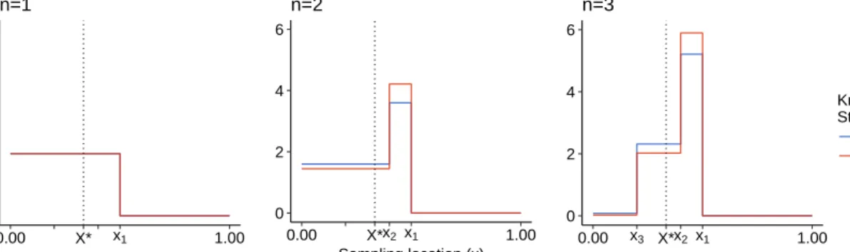
0 2 4 6 0.00 X* x1 1.00 n=1 0 2 4 6 0.00 X*x2 x1 1.00 Sampling location (x) n=2 0 2 4 6 0.00 x3 X*x2 x1 1.00 n=3 Knowledge State fn gn

Figure 2.3: True and approximated knowledge states with the empirical proportion estimator ¯pusing three sampling locationsx1:3 = (0.5,0.4,0.2) anda= 10, using the linear function (4.1) withx∗= 1/3.

The approximated posteriorfn+a differs relative to the true posterior gn+adue to the

fact that fn utilizes the estimated ˆp(xn+1) whereas gn uses the true p(xn+1). Figure 2.3

uses the majority proportion estimator ¯pto illustrate how the bias in ¯pinduces over/under confidence when comparing the knowledge state fn+a vis-a-vis the ground truth gn+a.

Starting with a f0, g0 ∼ Unif(0,1) prior, we compare the true posterior gn+a and its

approximation fn+a for n∈ {1,2,3}and a= 10, updated using the (arbitrary) locations

x1 = 0.5, x2 = 0.4 and x3 = 0.2 our running example (4.1). Note that the first two

sampling locations x1:2 are to the right ofx∗ = 1/3, whereasx3 is leftwards of x∗.

2.2.4 Aggregation of responses

An alternative strategy for updating the knowledge state is to build a subsidiary statistic from the i.i.d. (Yj(x))aj=1’s, whose specificity is boosted thanks to the batching.

In other words, instead of using the a-step update Ψ(·;p, a) with p, we utilize a 1-step update Ψ(·;P,1) with an adjusted probability of correct response P. In this case, we considermajority-vote statisticM(x) := 1{B(x)>da/2e} [37]. Then

(46)

Section 2.2 Knowledge States PM(p) :=Pp(M(x) = 1{x>x∗_}) = a X j=da/2e a j pj(1−p)a−j. (2.21)

Substituting an estimate ˆpin (2.21) then yields P_M(ˆp) =Pa j=da/2e a j ˆ pj₍₁₋_p)_ˆ a−j_{, and}

the boosted update rule

fn+K = Ψ fn, xn+1,M(xn+1);PM(ˆp(xn+1)),1

. (2.22)

Note that sinceM only uses limited information aboutB, it is not sufficient for learning p. Consequently, the resulting knowledge state is not directly comparable to the full Bayesian posterior gn; the hope is that through majority boosting we filter “noise” in B

and hence mitigate the bias in ˆp.

Aggregation of Functional Responses. Assuming that the functional responses (1.1) are available, another possibility for updating the knowledge state fn is to use the actual

functional values (Zj(x))aj=1 via the signal

S(x) := 1{Pa

j=1Zj(x)>0}. (2.23)

By the CLTP_S(h(x), σ(x)) :=_Ph,σ(S(x) = 1{x<x∗_})'Φ(

√

a|h(x)|/σ(x)), where σ2_(x)

is the location-dependent variance of (x). Observe that P_S(h(x), σ(x)) no longer de-pends on p(x) but on the signal-to-noise ratioh(x)/σ(x). A natural estimator forP_S is then PS(ˆha,σˆa) = Φ( √ a|ˆha(x)|/ˆσa(x)); (2.24) where ˆha:= _a1P_ja₌₁Zj and ˆσ2a := 1 a−1 Pa j=1(Zj−ˆha)

2 _{are the sample mean and variance}

obtained for a ≥ 2, respectively . Using the functional responses, the updated fn+a is

thus computed using S via

fn+a= Ψ

fn, xn+1,S(xn+1);PS(ˆha(xn+1),σˆa(xn+1)),1

(47)

Section 2.2 Knowledge States

Table 2.1: Schemes for knowledge state updatingfn+a based on query batches ofaat locationx.

Update Scheme Sufficient Statistic Parameters

p-estimate (2.10) using ¯por ˆp_L(¯p) B =Pa

j=11{Yj=+1} p

Majority Boosting (2.22) with P_M(ˆp) M = 1{B>da/2e} p

Functional Aggregation (2.25) withP_S(ˆha,σˆa) S = 1{Pa

j=1Zj>0} h/σ

TPO Strategy. A different aggregation ofZj’s relies on hypothesis testing,

specifi-callystatistical tests of power one (TPO) [55]. The key idea is to use an adaptive number of replicates aα(x) so as to boost the probability of correct response to levelpα, without

explicitly estimating p(x) [57]. Let S(x) := Pa

j=1Zj(x) and

aα(x) := min{k ∈N:|Sk(x)| ≥ck(α)}; (2.26)

where (ck(α))k∈_N is defined in terms of the distribution of (x) and the significance

parameter α ∈ (0,1). The adaptive batch size is aα and the resulting output is the

aggregated signal which is viewed as a test statistic for inference about the positiv-ity of the drift of the random walk S·(x). The construction of c·(α) guarantees that

˜

p(x) = _P( ˜Z(x) = sign(x∗ −x)) ≥ 1−α/2. To obtain the curved boundary c·(α)

re-quires knowledge of the distribution of Z(x). For example, if Z(x) ∼ N(h(x), σ2_{) then}

ck(α) = σ((n+ 1)[log(n+ 1)−2 logα])1/2.

Table 2.2 shows the average hitting time _Ep[aα(x)] as well as its estimated standard

deviation (in parentheses) for different p(x) (rows) and α (columns) combinations. It illustrates that the expected batch size grows exponentially as p(x) ↓ 1/2, which might be counterproductive in cases where the sampling budget is small. Indeed, instead of trying other locations, TPO will stubbornly sample the same x thousands of times.