APPLICATIONS OF SPIN GLASSES ACROSS DISCIPLINES: FROM COMPLEX SYSTEMS TO QUANTUM COMPUTING AND ALGORITHM
DEVELOPMENT
A Dissertation by ZHENG ZHU
Submitted to the Office of Graduate and Professional Studies of Texas A&M University
in partial fulfillment of the requirements for the degree of DOCTOR OF PHILOSOPHY
Chair of Committee, Helmut G. Katzgraber Committee Members, Stephen A. Fulling
Wolfgang Bangerth Winfried Teizer Head of Department, George R. Welch
August 2015
Major Subject: Physics
ABSTRACT
The main subjects of this dissertation are spin glass applications in other disci-plines and spin glass algorithms. Spin glasses are magnetic systems with disorder and frustration, and the essential physics of spin glasses lies not in the details of their microscopic interactions but rather in the competition between quenched ferromag-netic and antiferromagferromag-netic interactions. Concepts that arose in the study of spin glasses have led to applications in areas as diverse as computer science, biology, and finance, as well as a variety of others.
In the first part of this dissertation I study the equilibrium and non-equilibrium properties of Boolean decision problems with competing interactions on scale-free networks in an external bias (a magnetic field). First, I perform finite-temperature Monte Carlo simulations in a field to test the robustness of the spin-glass phase and I show that the system has a spin-glass phase in a field, i.e., it exhibits a de Almeida– Thouless line. Then I study avalanche distributions when the system is driven by a field at zero temperature to test whether the system displays self-organized critical-ity. The numerical results suggest that avalanches (damage) can spread across the entire system with nonzero probability when the decay exponent of the interaction degree is less than or equal to 2, i.e., that Boolean decision problems on scale-free net-works with competing interactions can be fragile when the system is not in thermal equilibrium.
In the second part of this dissertation I discuss the best-case performance of quantum annealers on native spin-glass benchmarks, i.e., how chaos can affect success probabilities. We perform classical parallel-tempering Monte Carlo simulations of the archetypal benchmark problem, an Ising spin glass, on the native chip topology.
Using realistic uncorrelated noise models for the D-Wave Two quantum annealer, I study the best-case resilience, or the probability that the ground-state configuration is not affected by random fields and random-bond fluctuations found on the chip. We compute the upper-bound success probabilities for different instance classes based on these simple error models, and I present strategies for developing robust and hard benchmark instances.
In the third part of this dissertation I present a cluster algorithm for Ising spin glasses that works in any space dimension and speeds up thermalization by several orders of magnitude at temperatures where thermalization is typically difficult. Our isoenergetic cluster moves are based on the Houdayer cluster algorithm for two-dimensional spin glasses and lead to a speedup over conventional state-of-the-art methods that increases with the system size. We illustrate the benefits (improved thermalization and achievement of more equiprobable sampling of ground states) of the isoenergetic cluster moves in two and three space dimensions, as well as in the nonplanar Chimera topology found in the D-Wave quantum annealing machine.
Finally, I study the thermodynamic properties of the two-dimensional Edwards-Anderson Ising spin-glass model on a square lattice using the tensor renormalization group method based on a higher-order singular-value decomposition. Our estimates of the partition function without a high precision data type lead to negative values at very low temperatures, thus illustrating that the method can not be applied to frustrated magnetic systems.
ACKNOWLEDGEMENTS
First and foremost I would like to thank my advisor, Dr. Helmut G. Katzgraber. It has been an honor to be his first Ph.D. student at Texas A&M University. He has taught me how to effectively communicate with other scientists and how to be efficient. I appreciate all of the time, ideas, and funding that he contributed to make my Ph.D. experience productive and meaningful. His enthusiasm for his research, for teaching, and for making excellent presentations have been motivational for me, and his high standards regarding writing quality, presentation skills, and professionalism have helped me to become more than a scientist and to make this dissertation possible.
The members of the computational physics group at Texas A&M have contributed immensely to my personal and professional development. The group has been a source of friendships as well as good advice and collaboration. I am especially grateful for Andrew Ochoa’s endless help with the English language and for his hospitality, which made office life more enjoyable and relaxed. It was Juan Carlos Andresen’s inspiring idea that allowed me to participate in the discovery of interesting science for the first time in my life. Ruben Andrist’s excellent programming skills set a strong example, showing me that I should study programming languages and become an efficient programmer. Visiting scholar Stefan Schnabel and postdoctoral researcher Oliver Melchert’s low-profile philosophy of life as a physicist earned my admiration. It was a pleasure to meet the great professors, staff, and graduate students at Texas A&M. Thanks to Dr. Stephen A. Fulling, Dr. Wolfgang Bangerth, and Dr. Winfried Teizer for serving as my committee members. Their time and effort were important for my Ph.D. research, not only in reviewing my dissertation, but also
by providing guidance and support for this work. I would like to thank Dr. Siu Chin and Chen Sun for their helpful discussions and suggestions concerning tensor network research. I would also like to thank graduate advisor Dr. Joseph Ross, Jill Lyster, Sandi Smith, and Sherree Kessler for their help with my course and degree plans.
Finally, I am truly and deeply indebted to my wonderful parents for their love, support, and encouragement throughout my entire life, and I am also very grateful to my friends Qi Zhang and Jinghui Wang.
TABLE OF CONTENTS
Page
ABSTRACT . . . ii
DEDICATION . . . iv
ACKNOWLEDGEMENTS . . . v
TABLE OF CONTENTS . . . vii
LIST OF FIGURES . . . x
LIST OF TABLES . . . xix
1. PHASE TRANSITIONS, CRITICAL PHENOMENA, SPIN GLASSES . . 1
1.1 Phase transitions . . . 1
1.2 Critical phenomena . . . 5
1.3 Spin glass . . . 9
1.3.1 Phase transitions in spin glasses . . . 10
1.3.2 Long-range and short-range spin glass model . . . 13
1.3.3 Applications of spin glasses . . . 15
2. NUMERICAL METHODS FOR SPIN GLASSES . . . 16
2.1 Metropolis algorithm . . . 17
2.2 Parallel tempering . . . 19
2.3 Houdayer cluster algorithm . . . 20
2.4 Test for equilibration . . . 22
2.5 Finite size scaling for spin glasses . . . 23
2.6 Optimization algorithms . . . 26
3. BOOLEAN DECISION PROBLEMS WITH COMPETING INTERAC-TIONS ON SCALE-FREE NETWORKS: EQUILIBRIUM AND NONEQUI-LIBRIUM BEHAVIOR IN AN EXTERNAL BIAS . . . 30
3.1 Model . . . 32
3.2 Equilibrium properties in a field . . . 33
3.2.2 Equilibration scheme and simulation parameters . . . 36
3.2.3 Numerical results for λ= 4.50 . . . 39
3.2.4 Numerical results for λ= 3.75 . . . 40
3.3 Nonequilibrium properties in a field . . . 45
3.3.1 Numerical details and measured observables . . . 46
3.3.2 Numerical results for Gaussian disorder . . . 48
3.3.3 Numerical results for bimodal disorder . . . 51
3.4 Summary and conclusions . . . 54
4. BEST-CASE PERFORMANCE OF QUANTUM ANNEALERS ON NA-TIVE SPIN-GLASS BENCHMARKS: HOW CHAOS CAN AFFECT SUC-CESS PROBABILITIES . . . 57
4.1 Model, observables and algorithm . . . 60
4.1.1 Model . . . 60
4.1.2 Instance classes and observables . . . 62
4.1.3 Algorithm details . . . 64
4.2 Results . . . 66
4.2.1 Yield of non-degenerate ground states . . . 66
4.2.2 Resilience to noise . . . 67
4.2.3 Effects of the number of first excited states . . . 69
4.3 Conclusions . . . 71
5. EFFICIENT CLUSTER ALGORITHM FOR SPIN GLASSES IN ANY SPACE DIMENSION . . . 74
5.1 Benchmark model and observables . . . 76
5.1.1 Reminder: Houdayer cluster algorithm . . . 77
5.1.2 Isoenergetic cluster algorithm . . . 79
5.2 Benchmarking results . . . 83
5.3 Summary . . . 87
6. EFFICIENT SAMPLING OF GROUND STATE CONFIGURATIONS FOR QUASI TWO-DIMENSIONAL ISING SPIN GLASSES . . . 89
6.1 Model, algorithm and observables . . . 90
6.2 Numerical results . . . 92
6.3 Conclusions . . . 97
7. LIMITATIONS OF APPLYING TENSOR RENORMALIZATION GROUP METHODS TO GLASSY SYSTEMS . . . 99
7.1 Model . . . 100
7.3 Numerical results . . . 102
7.3.1 Exact method . . . 102
7.3.2 HOTRG . . . 104
7.4 Conclusions . . . 107
8. SUMMARY AND OUTLOOK . . . 108
REFERENCES . . . 112
APPENDIX A. ANALYTICAL FORM OF THE DE ALMEIDA-THOULESS FORHR →0 . . . 133
LIST OF FIGURES
FIGURE Page
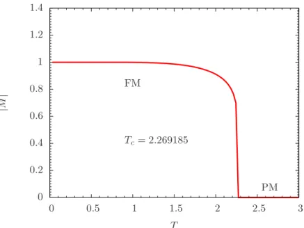
1.1 Sketch of phase diagram for water molecules, the blue curve represents the transition between liquid (water) and solid (ice) states, the red curve represents the transition between gas (vapor) and liquid (water) states, the purple curve represents the transition between solid (ice) and gas (vapor) states. . . 3 1.2 Magnetization as a function of temperature for the 2D Ising model. At
zero temperature, the state stays completely ordered. As we increase temperature, the magnetization starts to drop rapidly until the phase transition occurs. Above the critical temperature Tc = 2.269, the absolute magnetisation is nearly zero. . . 3 1.3 Disorder and frustration in a spin glass. Bonds marked “+”
corre-spond to ferromagnetic couplings, “-” correcorre-sponds to an antiferro-magnetic coupling. For a ferromagnet the energy is minimized by aligning all spins, in the case of spin glass, no spin configuration can simultaneously satisfy all couplings. . . 10 1.4 Sketch of phase diagram for three-dimensional Ising spin glass with
bimodal disorder. The blue curve represents the transition between ferromagnetic (FM) and paramagnetic states (PM), the purple curve represents the transition between spin glass (SG) and ferromagnetic states (FM), the red curve represents the transition between spin glass (SG) and paramagnetic states (PM). T and p are temperature and fraction of antiferromagnetic bonds, respectively. . . 11 1.5 Sketch of Almeida–Thouless (AT) line for the SK model. The AT
line separates a spin glass phase with divergent relaxation times and “replica symmetry breaking” from a paramagnetic “replica symmet-ric” phase with finite relaxation times. . . 15 2.1 Sketch of a rough energy landscape of spin glass. A Monte Carlo move
is unlikely if the height of the energy barrier ∆E is large, especially at low temperatures. In this case, a simple Monte Carlo simulation will stall and the system will be stuck in the metastable state. . . 18
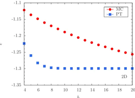
2.2 This figure shows energy per spin eas a function of Monte Carlo time (measured in lattice sweeps) t= 2b with (blue dots) and without (red dots) parallel tempering (system size N = 64, temperature T = 0.21) for a 2D square lattice. The system is in equilibrium whene becomes approximately flat and fluctuates around a mean value. The data show that without parallel tempering (PT), the system does not reach equilibrium even after 220 MCS. In contrast, the system thermalizes much faster with parallel tempering and reaches equilibrium after only a few thousand Monte Carlo sweeps. . . 20 2.3 This figure shows energy per spin e as a function of Monte Carlo
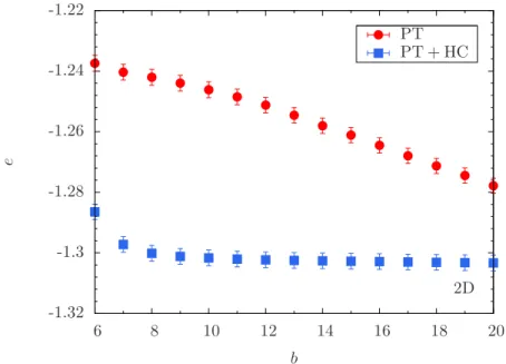
time (measured in lattice sweeps)t= 2b with (blue dots) and without (red dots) Houdayer cluster moves (system size N = 64, temperature T = 0.02) for a 2D square lattice. The system is in equilibrium when e becomes approximately flat and fluctuates around a mean value. The data show that without Houdayer cluster moves (HC), the system does not reach equilibrium even after 220MCS. However, it thermalizes much faster with Houdayer cluster moves and reaches equilibrium after only a few thousand Monte Carlo sweeps. Note temperatures for the simulations here are extremely low (about 1/10 of temperatures in figure 2.2), the simple Monte Carlo method will be useless. . . 22 2.4 Equilibration test for a 2D square lattice with N = 64 spins at T =
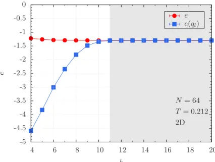
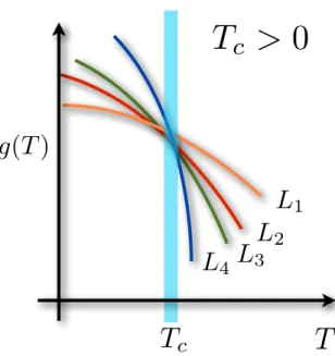
0.212. Once the data for the energye and the energy e(ql) computed from link overlapqlagree, the system is in thermal equilibrium (shaded area). . . 24 2.5 Sketch of Binder ratio g(T) for the Sherrington-Kirkpatrick model
with different system sizesN as a function of temperatureT. The data cross at a point (shaded area) and we obtain the critical temperature Tc. . . 25 2.6 Sketch of finite-size scaling analysis of Binder ratiog(T) for the
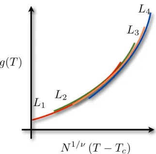
Sherrington-Kirkpatrick model with different system sizes N as a function of N1/ν(T −Tc). Close to the transition the data fall onto a universal curve, showing that ν is the correct value of the critical exponent. . 26
2.7 This figure [65] illustrates the relationships among the three categories: P, NP, and NP-complete. The existence of problems within NP but outside both P and NP-complete, under assumption P 6= NP, was established by Ladner’s theorem [66]. For spin glasses, non-planar model and the planar model with an external field are NP-complete, planar model is P, it is unclear whether there are spin glass problems that are in the complexity class NP but are neither in the class P nor NP-complete. . . 29 3.1 Equilibration test for N = 8192 spins at T = 1.500 (lowest
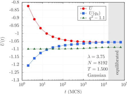
temper-ature simulated) and λ = 3.75. Once the data for the energy U and the energy computed from q4 [U(q4)] agree, the system is in thermal equilibrium (shaded area). At this point data forq2 are also indepen-dent of Monte Carlo time. Note that the data for q2 are shifted by a constant factor of 1.1 for better comparison. Error bars are smaller than the symbols. . . 37 3.2 Extrapolation to the thermodynamic limit for the critical temperature
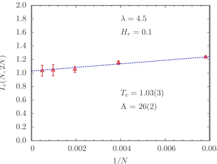
Tc for λ = 4.50 and Hr = 0.1. We determine the crossing points of critical temperatures of the susceptibility expression for pairs of system sizes N and 2N. Using Eq. (3.14) with ω = 1 we extrapolate the data to the thermodynamic limit. This allows us to take into account corrections to scaling in an unbiased way. . . 41 3.3 Field Hr versus temperature T phase diagram for an Ising spin glass
on a scale-free graph with λ = 4.50. The data points separate a paramagnetic (PM) from a spin-glass (SG) state. The shaded area is intended as a guide to the eye. The dotted (blue) line is a calculation of the AT line in theHr →0 limit. . . 42 3.4 Finite-size scaling analysis of χ/N2−η as a function of N1/ν(β −βc)
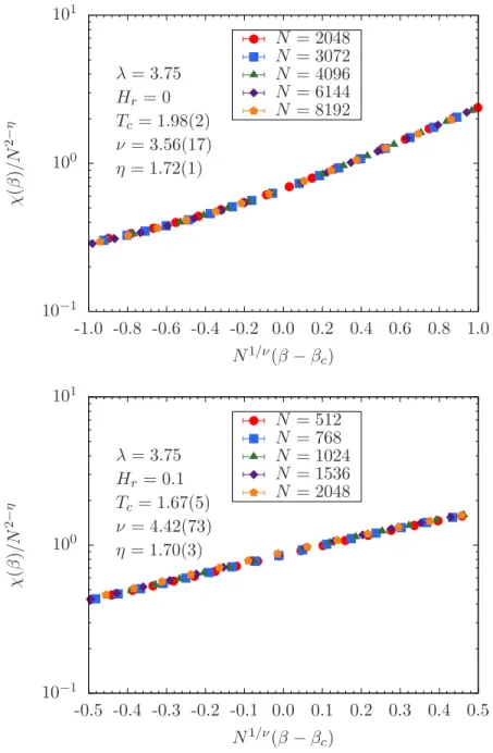
for an Ising spin glass on a scale-free network with Gaussian disorder and λ = 3.75. The data at zero field (top panel) scale very well. The bottom panel shows representative data forHr = 0.1 scaled according to Eq. (3.7). Error bars are smaller than the symbols. . . 44
3.5 Field Hr versus temperature T phase diagram for an Ising spin glass on a scale-free graph with λ = 3.75. The data points separate a paramagnetic (PM) from a spin-glass (SG) state. The shaded area is intended as a guide to the eye. The dotted (blue) line is a calculation of the AT line in theHr →0 limit. Note that estimates for the critical temperature Tc from a finite-size scaling analysis (FSS) according to Eq. (3.7) withTc, η, and ν as free parameters agree within error bars with estimates at finite fields whereη = 19/11 and ν= 11/3 are used as fixed parameters (labeled with “Fixed” in the plot). . . 45 3.6 Top: Avalanche distribution D(n) for the Edwards-Anderson
spin-glass model with Gaussian disorder on scale-free networks with λ = 4.50 recorded across the whole hysteresis loop. The data show no system size dependence. The vertical (black) line marks the extrap-olated value of n∗. Clearly, no signs of SOC are visible in the data. Bottom: Magnetization M = (1/N)P
isi versus field H hysteresis loop forλ= 4.50 and 48000 spins. The data are for one single sample and meant as an illustration for the typical behavior of the system in a field. The inset shows a zoom into the boxed region. The discrete steps due to magnetization jumps in the hysteresis loop are clearly visible. . . 49 3.7 Top: Avalanche distribution D(n) for the Edwards-Anderson
spin-glass model with Gaussian disorder on scale-free networks withλ= 1.5 recorded across the whole hysteresis loop. For λ = 1.5 < 2.0 the number of neighbors diverges. The data show a clear system-size de-pendence with the distributions becoming increasingly power-law-like for increasing system size N. As shown in Fig. 3.8, the extrapolated cutoff value is n∗ = ∞, i.e., the system exhibits true SOC behavior. Bottom: Magnetization M = (1/N)P
isi versus field H hysteresis loop forλ= 1.50 and 48000 spins. The data are for one single sample and meant as an illustration for the typical behavior of the system in a field. The inset shows a zoom into the boxed region. The discrete steps due to magnetization jumps in the hysteresis loop are clearly visible. Qualitatively, the data seem to show larger rearrangements as for λ= 4.50 (Fig. 3.6). . . 50 3.8 Characteristic avalanche size n∗ extrapolated to the thermodynamic
limit for different values ofλ and Gaussian disorder. Plotted are 1/n∗ versus λ. Only when 1/n∗ = 0 (here within error bars) we can expect the system to show SOC behavior. This is only the case for λ ≤ 2, i.e., in the regime where the number of neighbors diverges. . . 51
3.9 Avalanche distributionD(n) for the Edwards-Anderson spin-glass model with bimodal disorder on scale-free networks with λ = 3.5 recorded across the whole hysteresis loop. Top panel: Data for p = 0.63< pc. Here the system displays subcritical behavior, i.e., the characteristic avalanche sizen∗ is finite. Center panel: For p= 0.66≈pcthe system is in the critical regime where the distributions are well described by power laws. Bottom panel: For p = 0.70 > pc the system is in the supercritical regime. A jump in the hysteresis loop occurs, i.e., very large rearrangements are very probable, as can be seen in the bump that develops in the distributions D(n) for largen. . . 52 3.10 Fraction of ferromagnetic bonds p versus λ phase diagram for the
Edwards-Anderson spin-glass model on scale free networks with bi-modal interactions between the spins. For λ > 2 a critical line pc(λ) separates the subcritical regime where avalanches are small, from the supercritical regime where system-spanning avalanches are very com-mon. Along the critical line pc(λ) (triangles, solid line) avalanche sizes are distributed according to power laws. For λ ≤2 the number of neighbors diverges. In this regime for p= 0.5 the system displays avalanches that are power laws, i.e., true SOC. The dotted line repre-sents the spin-glass–to–ferromagnetic phase boundary from Fig. 2 in Ref. [2]. . . 55 4.1 Adjacency matrix of the D-Wave Two chip with 8×8 K4,4 cells and
512 qubits (circles) connected by couplers (lines). . . 61 4.2 Resilience (R) of different instance classes (see text) for a N = 512
qubit system on the Chimera graph as a function of Gaussian random field strength (h). Instance classes are less resilient to noise with increasing field strength and decreasing classical energy gap. The shaded line represents the current field noise strength of approximately 5% in the D-Wave Two system. . . 68 4.3 Resilience (R) of different instance classes (see text) for a N = 512
qubit system on the Chimera graph as a function Gaussian random bond fluctuation strength (∆J). Instance classes are less resilient to noise with increasing bond fluctuation strength and a decreasing classical energy gap. The shaded line represents the current bond noise strength in the D-Wave Two system, i.e., ∼ 3.5%. Note that bond noise has a stronger effect than field noise (Fig.4.2) on the device. 69
4.4 Resilience R of the U5,6,7 instance class as a function of the bond fluctuation strength (∆J) for different system sizesN on the Chimera topology. The resilience clearly decreases for increasing noise and system size. The shaded vertical line represents the current bond-noise strength in the D-Wave Two system, approximately 3.5%. . . . 70 4.5 Resilience R as a function of the number of first excited statesN1 for
N = 512 spins on the Chimera lattice. The data are for the U5,6,7 instance class. The color bar shows approximately how often a given number of first excited states occurs for the 900 instances studied. In this case, between four and eight first excited states are most common. 71 5.1 Fraction of spins pof potential cluster members as a function of
tem-peratureT for different system sizes N in two space dimensions (2D). The horizontal line represents the percolation threshold of a two-dimensional square lattice, i.e., pc ≈ 0.592 [156]. Because p → 0.5 for T → ∞, for all T clusters do not percolate, which is why the HCA is efficient in two-dimensional planar geometries. Error bars are computed via a jackknife analysis over configurations and are smaller than the symbols. . . 80 5.2 Fraction of spinspas a function of temperatureT for different system
sizes N on the Chimera topology. The horizontal line represents the percolation threshold of the nonplanar Chimera topology, namelypc≈ 0.387 computed here using the approach developed in Ref.[157]. For T & J = 1 clusters percolate and cluster updates provide no gain. Error bars are computed via a jackknife analysis over configurations and are smaller than the symbols. . . 81 5.3 Fraction of spinspas a function of temperatureT for different system
sizes N in three space dimensions (3D). The horizontal line repre-sents the percolation threshold of the three-dimensional cubic lattice (pc ≈0.311 [158]). For T &J = 1 clusters percolate. Error bars are computed via a jackknife analysis over configurations and are smaller than the symbols. . . 82 5.4 ∆ [Eq. (5.4)] as a function of simulation time t = 2b measured in
Monte Carlo sweeps in two space dimensions (2D) for N = 1024 and T = 0.212. Simulations using vanilla PT thermalize at at least 225 Monte Carlo sweeps, whereas with the addition of ICMs thermaliza-tion is reduced to approximately 216Monte Carlo sweeps. This means approximately two orders of magnitude improvement. Error bars are computed via a jackknife analysis over configurations. . . 84
5.5 ∆ as a function of simulation time t = 2b measured in Monte Carlo sweeps for an Ising spin glass on Chimera with N = 1152 spins at T = 0.212. Simulations using PT thermalize at approximately 225 Monte Carlo sweeps, whereas the addition of ICMs reduces thermal-ization to 218Monte Carlo sweeps. Again, approximately two orders of magnitude speedup. Error bars are computed via a jackknife analysis over configurations. . . 85 5.6 ∆ as a function of simulation time t = 2b measured in Monte Carlo
sweeps in three space dimensions (3D) for N = 1728 and T = 0.42∼ 0.43Tc. Using standard PT, the system thermalizes approximately after 223 Monte Carlo sweeps. This time is reduced to ∼ 220 Monte Carlo sweeps when ICMs are added. Error bars are computed via a jackknife analysis over configurations. . . 86 5.7 Ratio between theapproximateaverage thermalization time of PT and
PT+ICM for different topologies at the lowest simulation temperature (see Tab. 5.1) as a function of system sizeN. In all cases the speedup increases with increasing system size. Note that thermalization times have been determined by eye. . . 87 6.1 Scatter plot of quantities Qnum√n as a function of the ground state
degeneracyG−1 for different spin glass samples with different system sizesN on a Chimera graph. The data points for ICA (blue color) are closer to the theoretical limit than those for the PT (red color), and this improvement gets better as the system size increases. . . 93 6.2 Median ratioQnum/Qth over different spin glass samples as a function
of the system sizeN on a Chimera graph. The data points show that ICA (blue color) is better than PT (red color) for all system sizes, and the general trend for both algorithms is that the ratio goes up as the system size increases, then it peaks at a certain point, and beyond a certain system size the ratio goes down as the system size continues to increase. Note there is no critical point and phase transition here. 94
6.3 Two examples of ground state configurations with different Hamming distances on a Chimera graph for system sizeN = 512. The Hamming distance denotes the difference between two binary strings (ground state configurations). Each dot in the figure represents a ground state, black lines are 1-bit differences, red lines are 2-bit differences, and anything that is a light color or blue is an even greater difference. In the example on the left, all ground state configurations are related by 1-bit differences, while the example on the right shows that Hamming distances between certain ground state configurations can be large— which means that it will take longer for the system to move from one ground state to another and this will cause larger fluctuations in the ground state frequency. . . 95 6.4 Scatter plot of quantities Qnum√n as a function of the ground state
degeneracyG−1 for different spin glass samples with different system sizes N on a 2D lattice. The data points for ICA (blue color) are closer to the theoretical limit than those for the PT (red color), and this improvement gets better as the system size increases. . . 96 6.5 Median ratioQnum/Qth over different spin glass samples as a function
of the system size N on a 2D lattice. The data points show that ICA (blue color) is better than PT (red color) for all system sizes, and the general trend for both algorithms is that the ratio goes up as the system size increases, then it peaks at a certain point, and beyond a certain system size the ratio goes down as the system size continues to increase. Note there is no critical point and phase transition here. 97 7.1 Failure rate Pf of the partition function for 2D Edwards-Anderson
spin glass as a function of the temperatureT. 960 samples with L= 4 and p= 0.5 were generated to calculate the failure rate and error bars. 102 7.2 Failure rate Pf of the partition function for 2D Edwards-Anderson
spin glass as a function of the number of bits B. 960 samples with L= 4 and p= 0.5 atT = 0.05 were generated to calculate the failure rate and error bars. . . 104 7.3 Example plot for 256 tensor components of 2D Edwards-Anderson
spin glass with p = 0.5, L = 4, and T = 0.05 and components of the ferromagnetic Ising model with L = 4 and T = 0.05. Tf is the tensor element value and If is the tensor element index of the final contracted tensor. . . 105
7.4 Failure ratePf of the partition function for 2D Edwards-Anderson spin glass with HOTRG as a function of the temperature T and number of bits B. 480 samples with L = 4,8,16 and p= 0.5 were generated to calculate the failure rate and error bars. . . 106
LIST OF TABLES
TABLE Page
1.1 Different orders of phase transitions. First-order phase transitions are those that involve a latent heat. Second-order phase transitions are also called continuous phase transitions and characterized by a divergent susceptibility, an infinite correlation length, and a power-law decay of correlations near criticality. . . 5 3.1 Parameters of the simulation: For each exponentλand system sizeN,
we compute Nsa disorder or network instances. Nsw = 2b is the total number of Monte Carlo sweeps for each of the 4NT replicas for a single instance, Tmin [Tmax] is the lowest [highest] temperature simulated, and NT is the number of temperatures used in the parallel tempering method for each system size N. . . 38 3.2 Critical parameters Tc, ν, and η for a spin glass with Gaussian
ran-dom bonds defined on a scale-free graph. The data forλ = 4.50 have been determined using the mean-field finite-size scaling expression in Eq. (3.9). In this case one can, in principle, defineη= 5/3 and ν = 3, although these should be viewed as parameters placed in Eq. (3.7) to obtain Eq. (3.9). For λ = 3.75 we determine the critical param-eters using Eq. (3.7). The starred estimates of Tc for Hr > 0 have been determined by using the zero-field estimates of η = 19/11 and ν = 11/3 as fixed. BothTcand Tc? agree within error bars, except sta-tistical fluctuations are smaller for Tc? because there are fewer fitting parameters. . . 43 3.3 Simulation parameters in the nonequilibrium study with both
Gaus-sian and bimodal-distributed random bonds: For each exponentλ we study systems of N = 500×2m spins with m ∈ {1, . . . , mmax}. For Gaussian disorder, when λ <4, we also simulate systems with 48 000 spins (m= 6 corresponds to 32 000 spins). All distributions are com-puted using Nsa disorder realizations. . . 47
4.1 Simulation parameters: For each instance class and system sizeN, we compute Nsa instances. Nsw = 2b is the total number of Monte Carlo sweeps for each of the 4NT replicas for a single instance,Tmin [Tmax] is the lowest [highest] temperature simulated, and NT is the number of temperatures used in the parallel tempering method. For the lowest Nicm temperatures isoenergetic cluster moves are applied. . . 66 5.1 Parameters of the simulation in two space dimensions (2D), three
space dimensions (3D), and on the Chimera (Ch) topology. For each topology simulated and system sizes N, we compute Nsa disorder in-stances and measure over 2b Monte Carlo sweeps (and isoenergetic cluster moves) for each of the 2NT replicas. Tmin [Tmax] is the low-est [highlow-est] temperature simulated, and NT is the total number of temperatures used in the parallel tempering Monte Carlo method. Isoenergetic cluster moves only occur for the lowest Nc temperatures simulated (determined from figs. 5.1 to 5.3). . . 84 6.1 Parameters of the simulation: For each instance class and system size
N, we compute Nsa instances. Nsw = 2b is the total number of Monte Carlo sweeps for each of the 4NT replicas for a single instance, Tmin [Tmax] is the lowest [highest] temperature simulated, and NT and Nhc are the number of temperatures used in the parallel tempering method and in the isoenergetic cluster algorithm, respectively. . . 92
1. PHASE TRANSITIONS, CRITICAL PHENOMENA, SPIN GLASSES
The analysis of phase transitions and the associated microscopic structures is a well-developed scientific approach in physics. Mathematical and conceptual tools developed from spin glass phase transition have found their way into a variety of ap-plications, including satisfiability problem [1], probability of finding an unsatisfiable instance shows a sharp threshold behavior at some critical ratio between the number of clauses and variables; the robustness of scale free network to local perturbation [2]; the finite-temperature phase space of quantum annealer [3]; percolation theory [4]; etc. In this chapter we provide an overview of phase transition, critical phenomena and spin glass physics.
1.1 Phase transitions
A phase transition is the transformation of a thermodynamic system from one phase to another. A phase is a state of matter in which the macroscopic physical properties of the substance are uniform on the macroscopic scale and usually charac-terized by a thermodynamic function, which is a function of macroscopic parameters such as temperature, pressure, etc. During a phase transition of a thermodynamic system, certain properties of the system change as a result of a change in some macroscopic parameters. For example, a liquid may become gas when heated to the boiling point, resulting in an abrupt change in volume, and a two-dimensional (2D) Ising model [5] may suddenly lose its spontaneous magnetization as its temper-ature exceeds the critical tempertemper-ature. These properties of the system are actually measures of the degree of order across boundaries in the phase transition and are usually called order parameters. From a theoretical point of view, order parameters arise from symmetry breaking; for example, in the case of the 2D Ising model, the
magnetization M is spontaneously broken when the system is cooled to below the Curie temperature.
A phase diagram is a graphical representation of the physical states of matter under different conditions indicated by the macroscopic parameters. A typical phase diagram has macroscopic parameters on the x- and y-axes and several specific fea-tures, including phase boundaries, a critical point, and a triple point. A phase boundary separates different phases. A change in parameters across a phase bound-ary, such as a change in temperature, causes a sudden change in the phase of the substance. A phase boundary sometimes disappears at a critical point, where the two phases become indistinguishable and the substance shows anomalous behavior.
Figure 1.1 below shows a phase diagram for water molecules. Every point in this diagram represents a possible combination of temperature and pressure for the system. The diagram is divided into three areas, which represent the solid, liquid, and gas states of the water molecules.
Figure 1.2 shows a phase diagram for the 2D Ising model using Onsager’s formula for spontaneous magnetization. There is a phase transition at the critical tempera-ture Tc = 2.269J/k: the system stays mostly ordered below the critical temperature and the average magnetization M is one, while the system becomes completely un-ordered above Tc and the average magnetizationM is zero.
In the conventional classification [6], phase transitions are divided into two broad categories by the degree of singularity in the physical quantities (see table 1.1). When the first-order derivative of the free energy (usually either Helmholtz free energyF or Gibbs free energyG) shows a discontinuity, the transition is first-order and typically involves latent heat. The transition is called continuous if the second- or a higher-order derivative of the free energy shows a discontinuity or divergence. Continuous phase transitions are usually characterized by a divergent susceptibility, an infinite
Gas Liquid
Solid
T P
Figure 1.1: Sketch of phase diagram for water molecules, the blue curve represents the transition between liquid (water) and solid (ice) states, the red curve represents the transition between gas (vapor) and liquid (water) states, the purple curve represents the transition between solid (ice) and gas (vapor) states.
0 0.2 0.4 0.6 0.8 1 1.2 1.4 0 0.5 1 1.5 2 2.5 3 | M | T Tc = 2.269185 FM PM
Figure 1.2: Magnetization as a function of temperature for the 2D Ising model. At zero temperature, the state stays completely ordered. As we increase temperature, the magnetization starts to drop rapidly until the phase transition occurs. Above the critical temperature Tc= 2.269, the absolute magnetisation is nearly zero.
correlation length, and a power-law decay of correlations near criticality. Examples of first-order phase transitions are the melting of ice and the boiling of water. The ice–water or water–vapor transition releases latent heat, which means that entropy
S =−∂F
∂T (1.1)
is discontinuous. Alternatively, we can say that volume
V = ∂G
∂P (1.2)
is discontinuous. An example of a second-order phase transition is in the 2D Ising model, where the specific heat
Cv =T( ∂S
∂T)v =−T( ∂2F
∂T2)v (1.3)
and magnetic susceptibility
χ= ∂m ∂H =−
∂2F
∂H2 (1.4)
are divergent at the critical temperature.
In some limited cases, we can derive exact solutions for the phase transitions of a thermodynamic system—for instance, in the case of 1D and 2D Ising models [7, 5]. But in general, we have to resort to approximate methods to understand phase transitions. Mean field theory was introduced by Landau [8, 9] in an attempt to formulate a general theory of continuous phase transitions. Essentially, mean field theory neglects spin fluctuations around the mean and treats spins as behaving statistically independently. In the simplest version, when Weiss mean field theory predicts the existence of a phase transition for the 1D Ising model, it fails even
qualitatively. However, in higher dimensions, spin is coupled with more and more neighbors, whose fluctuations around the mean magnetization will increasingly tend to cancel one another. Thus, mean field theory gives the correct results for an Ising model with a high enough space dimension (D= 4 is the upper critical dimension).
Table 1.1: Different orders of phase transitions. First-order phase transitions are those that involve a latent heat. Second-order phase transitions are also called con-tinuous phase transitions and characterized by a divergent susceptibility, an infinite correlation length, and a power-law decay of correlations near criticality.
Differential of free energy G Corresponding experimental quantities
First S, V S, V Second (∂T∂S)p,(∂V∂T)p,(∂S∂p)T,(∂V∂p)T Cp, β, κ Third ( ∂2S ∂T2)p,(∂ 2V ∂T2)p, ∂ 2S ∂T ∂p ( ∂Cp ∂T )p,( ∂β ∂T)p,( ∂κ ∂T)p (∂∂p2S2)T,( ∂2V ∂p2)T, ∂2V ∂T ∂p ( ∂Cp ∂p )T,( ∂β ∂p)T,( ∂κ ∂p)T 1.2 Critical phenomena
Critical phenomena [10] often refers to continuous phase transitions; it is the collective name associated with the physics of critical points. The critical behavior is usually different from the mean-field approximation that is valid away from the phase transition. This is because the mean-field approximation neglects correlations, which become increasingly important as the system approaches the critical point where the correlation length diverges. The three pillars of modern critical phenomena theory are scaling, universality, and renormalization [10].
The scaling hypothesis [11, 12] has two categories of predictions, both of which have been remarkably well verified by experimental data for diverse systems. The first category is a set of relations, called scaling relations, that serve to relate the various critical-point exponents, which describe the behavior of physical quantities
near continuous phase transitions. For example, the critical exponents of phase transitions in the Ising model, α, β, γ, and ν, describe the behavior of the specific heat Cv, the magnetization M, the susceptibility χ, and the correlation length ξ, respectively:
Cv ∼t−α, (1.5)
M ∼t−β, (1.6)
χ∼t−γ, (1.7)
ξ∼t−ν, (1.8)
wheret is reduced temperature t= (T −Tc)/Tc. These Ising critical exponents obey the scaling relations
α+ 2β+γ = 2, νd= 2−α. (1.9)
These equations imply that there are only two independent exponents. The second scaling hypothesis category is data collapse, which can also be explained using the Ising model. The ratio
ξ/L=t−νL−1 (1.10)
should control the behavior of finite-size data close to Tc. Assume thatχ(t) has the finite-size scaling form
χ(t)∼Lσf(ξ/L) =Lσf(t−νL−1) =Lσg(tL1/ν) (1.11)
for small t, then the infinite L scaling form should be
To reproduce this, the scaling functiong(x) must have the limitg(x)∼xb asx→ ∞. We can determine the exponents as follows:
χ(t)∼Lσg(tL1/ν) =Lσ(tL1/ν)b =tbLσ+b/ν, (1.13)
so b=−γ, σ=γ/ν,and
χ(t)∼Lγ/νC(tL˜ 1/ν). (1.14) Similarly, for the magnetization:
M(t)∼Lβ/νM˜(tL1/ν). (1.15)
Here ˜C and ˜M are unknown scaling functions. Both scaling forms show that when T =Tc, the data forχ(t)/Lγ/ν and M(t)/Lβ/ν simulated for different system sizesL should cross in the large-Llimit at T =Tc.
The concept of a universality class is the centerpiece of the modern theory of critical phenomena. Two systems with the same critical exponent values and scal-ing functions are said to belong to the same universality class. Data collapse onto a scaling function supports the scaling hypotheses, while the fact that the scaling function is the same for different materials is truly remarkable. For example, the critical exponents of the 3D Ising model phase transitions are the same as those at the liquid–gas critical point, and they share the same Ising model universality class with α = 0.110(1), β = 0.3265(3), γ = 1.2372(5), and ν = 0.6301(4). Universality is a prediction of renormalization group theory, which states that the thermody-namic properties of a system near a critical point depend only on dimensionality and symmetry and are insensitive to the underlying microscopic properties of the system. The idea of a renormalization group (RG) stems from Wilson’s [13] essential
idea that the critical point can be mapped onto a fixed point of a suitably chosen transformation on the system’s Hamiltonian. Here is an example of how to develop a real-space RG for the 1D Ising model. The energy E of the 1D Ising model is
H=−JX i
sisi+1 (1.16)
and the partition function is
Z =X {si} e−H/k =X {si} Y i eKsisi+1, (1.17)
whereK =J/kT. One way to reduce the number of degrees of freedom is to describe the system in terms of two-spin cells, where the partition function is written as
Z = Tr(TN) = Tr(T2)N/2 = Tr(T0)N/2 (1.18) with T0 = e2K+e−2K 2 2 e2K+e−2K . (1.19)
If we require T0 to have the same form as T, then
T0 =C eK0 e−K0 e−K0 eK0 . (1.20)
The solution to this matrix equation is recurrence relations
K0 = 1
and
C4 = 4(e4K +e−4K+ 2). (1.22) Suppose we have some initial value of the coupling constant K0 such that 0< K0 < 1. Then iteration of the recurrence relation produces a succession of values that approach K = 0. Accordingly, the point corresponding to K = 0 is called a stable fixed point of the recurrence relations, or a critical point of the 1D Ising model phase transition. This renormalization group description provides a foundation for understanding the scaling and universality, a calculation tool that permits us to obtain numerical estimates for the various critical exponents.
1.3 Spin glass
Spin glasses [14] are magnetic systems with disorder and frustration. The bonds in a spin glass are a mixture of roughly equal numbers of ferromagnetic bonds and antiferromagnetic bonds, and the essential physics of spin glasses lies not in the de-tails of the microscopic interactions but rather in the competition between quenched ferromagnetic and antiferromagnetic interactions shown in Figure 1.3. The Hamil-tonian H for a spin glass can be described as follows:
H=−X
i,j
JijSiSj +X i
hiSi, (1.23)
whereJij denotes the interactions between spins andSi denotes the values of the spin components. If Si has a single component, it’s called an Ising spin glass. If Si has two or three components, it is called anXY or a Heisenberg spin glass, respectively. A characteristic feature of spin glasses is that their dynamics are very slow at low temperatures, due to the development of a complicated “energy landscape” with many valleys separated by barriers.
Disorder Frustration
−
+
+
+
?
+
+
+
+
Spin glass FerromagnetFigure 1.3: Disorder and frustration in a spin glass. Bonds marked “+” correspond to ferromagnetic couplings, “-” corresponds to an antiferromagnetic coupling. For a ferromagnet the energy is minimized by aligning all spins, in the case of spin glass, no spin configuration can simultaneously satisfy all couplings.
1.3.1 Phase transitions in spin glasses
Unlike a ferromagnet, where thermal fluctuations completely eliminate sponta-neous magnetization above the critical temperature, spin glasses intrinsically do not have a visible spatial order. The spins in a spin glass are frozen with random orienta-tions at low temperatures, and a spin overlap comparing two copies of a system with the same disorder rather than magnetization plays the role of the order parameter. We compute the spin overlap via two independent replicas at the same temperature as qαβ = 1 N X i SiαSiβ. (1.24)
Above a spin glass’s critical temperature Tc, the spins fluctuate widely and the overlap parameter tends to be zero. Below the critical temperature Tc, the spins are frozen with random orientations and the overlap parameter is one (or minus one). Spin glasses exhibit continuous phase transitions, and the specific heat Cv has a broad, smooth, and rounded maximum. However, the non-linear susceptibility χnl diverges at the critical temperature Tc. χnl can be measured experimentally and is
SG FM
PM
p T
Figure 1.4: Sketch of phase diagram for three-dimensional Ising spin glass with bi-modal disorder. The blue curve represents the transition between ferromagnetic (FM) and paramagnetic states (PM), the purple curve represents the transition be-tween spin glass (SG) and ferromagnetic states (FM), the red curve represents the transition between spin glass (SG) and paramagnetic states (PM). T and pare tem-perature and fraction of antiferromagnetic bonds, respectively.
defined by the coefficient of h3 in the expansion of the magnetization m:
m =χh−χnlh3. (1.25)
The non-linear susceptibilityχnlis essentially the same as the spin glass susceptibility χSG: χSG = 1 N X i,j [hSiSji2]av. (1.26) where [· · ·]av denotes an average over the quenched disorders. For the Edwards-Anderson model, it can be shown that
T3χnl =χSG−2/3. (1.27)
computed from the spin glass correlation function due to Ornstein-Zernicke approx-imation
[χSG(0)/χSG(k)]−1 ≈1 +ξ2k2, (1.28) where χSG(k) is the vector-dependent spin glass susceptibility
χSG(k) = 1 N X i,j [hSiSji2]aveik·(Ri−Rj) (1.29)
and R is position vector. On a finite lattice the momentum is discretized and one arrives at the expression
ξ= 1 2 sin(kmin/2) χSG(0) χSG(kmin)− 1 !1/2 (1.30) with kmin= 2π L(1,0,0). (1.31)
The phase diagram of the 3D lattice ±J Ising spin glass model is sketched in figure 1.4. p is the fraction of antiferromagnetic bonds, we only consider p ≤ 1/2 because of the symmetry p → 1−p. While the high-temperature phase is always paramagnetic (PM), at low temperatures there is a ferromagnetic (FM) phase for small frustration, and a spin glass phase (SG) with vanishing magnetization for sufficiently large frustration.
The critical exponents of phase transitions in spin glasses,α, β, γ,andν, describe the behavior of the specific heat Cv, overlap parameter q, susceptibility χSG, and correlation length ξL, respectively:
q∼t−β, (1.33)
χSG∼t−γ, (1.34)
ξ∼t−ν. (1.35)
This allows us to study critical properties and universality class in spin glasses via scaling relations.
1.3.2 Long-range and short-range spin glass model
For the Sherrington-Kirkpatrick (SK) model [15], a system ofN Ising spins with zero external fields and the range of each interaction can be infinite (every spin interacts with every other one). the Hamiltonian is described as follows:
H=−√1 N
X
i,j
JijSiSj. (1.36)
The couplings Jij are chosen from a Gaussian distribution with mean zero and vari-ance one; the √1
N rescaling ensures a non-divergent thermodynamic limit for free energy per spin as well as other thermodynamic quantities. The equilibrium solution of the model was found by Giorgio Parisi with the replica method, and subsequent work on the interpretation of the Parisi solution revealed the complex nature of a glassy low temperature phase characterized by ergodicity breaking, ultrametricity, and non-self-averageness [16, 17, 18, 19]. The SK model has a line of transitions, known as the Almeida–Thouless (AT) line (shown in Figure 1.5), in a magnetic field. The AT line separates a spin glass phase with divergent relaxation times and “replica symmetry breaking” from a paramagnetic “replica symmetric” phase with finite re-laxation times. Therefore, the SK model has a finite-temperature spin-glass phase transition in a field.
In the Edwards-Anderson model [20], spins are arranged on a D-dimensional lattice with only nearest neighbor interactions and periodic boundary conditions in all directions. Its Hamiltonian is
H=−X
i,j
JijSiSj, (1.37)
where i, j indicates a sum over nearest neighbors. The coupling constants Jij are independent random variables drawn from a given distribution with mean zero and variance one. In the original version proposed by Edwards and Anderson, the spin was assumed to be the Heisenberg one with three spin components. However, Ising spin glasses have been widely used in numerous simulations because of their sim-plicity. Much of what we know about the Edwards-Anderson model comes from numerical simulations, and there has been a general consensus that for Ising systems with D ≥ 2.5 [21], a spin glass transition occurs in zero field. The upper critical dimension of the Ising spin glass, above which mean field results should apply, is expected to be six [22]. Phase transitions in the magnetic field for the Edwards-Anderson model are controversial, and two main scenarios have been proposed for resolving this issue. In the “droplet picture” [23, 24, 25], there is no AT line in any finite-dimensional spin glass. By contrast, the “replica symmetry breaking” picture [26, 27] predicts that the behavior of short-range Ising spin glasses is similar to that of the infinite-range SK model with an AT line. Many problems can be mapped onto short-range systems. As such, whether having a field term could destroy the spin glass state has far-reaching impact [28]. Most of recent numerical studies point to the absence of an equilibrium transition under finite fields [28, 29], however, there is still no consensus on this issue because there seem to be quite large corrections to finite-size scaling. Therefore, better models such as one-dimensional spin-glass model
with power-law interactions and spin glasses on scale free networks can be used to probe short-range models by tuning the exponent of the power-law interactions or the exponent that describes the decay of the interaction degree in the scale-free graph [30, 31].
T H
SG
PM
Figure 1.5: Sketch of Almeida–Thouless (AT) line for the SK model. The AT line separates a spin glass phase with divergent relaxation times and “replica symme-try breaking” from a paramagnetic “replica symmetric” phase with finite relaxation times.
1.3.3 Applications of spin glasses
The study of spin glasses has led to a variety of applications to problems in neural networks [32], graph theory [33, 2], protein folding [34], self-organized criticality [35], combinatorial optimization [36], quantum information theory [37, 38, 3], economics [39], and many other areas. In this thesis, I attempt to illustrate how the spin glass model can establish fruitful links and contribute new insights to a wide range of interdisciplinary applications.
2. NUMERICAL METHODS FOR SPIN GLASSES
For a spin glass system in equilibrium with a heat bath, the probability Ps of being in a given state s depends only on the energy Es:
Ps = 1 Ze
−Es/kT. (2.1)
wherek is Boltzmann constant,T is the temperature andZ is the partition function of the system. To sample the average of an observable hOi in the system, we sum over all possible configurations analytically:
hOi= 1 Z
X
s
Ose−Es/kT. (2.2)
For a system with N spins, there are a total of 2N possible configurations. Even a small lattice with N = 100 is impossible to study using “brute force”, especially systems with strong interactions between spins. We have no choice but to seek an approximation if we want to correctly estimate the observables without exploring the entire configuration space. Unlike the case of ferromagnets, which display spa-tial symmetries that greatly simplify their physical and mathematical analyses, the absence of symmetries in spin glasses enormously complicates the analysis of their behavior. Mean field theory has almost always served as an invaluable guide to the low-temperature behavior of statistical mechanical systems. However, in the Edwards-Anderson model, there are finite corrections to the mean field (especially large in one or two dimensions). Because of this failure of mean field theory to pro-vide a correct description of the low-temperature phase in any finite dimensional spin glass [14, 40, 41], it is necessary to develop efficient numerical algorithms—especially
for those cases where exact results such as critical temperature, critical exponents, avalanche size distributions, and ground states are not available, due to formidable mathematical difficulties and NP-hard complexity. Over the last few decades, the development of efficient Monte Carlo methods such as parallel tempering [42] and population annealing [43] has helped us understand these systems at a much deeper level. However, most numerical studies are still plagued by corrections to finite-size scaling due to the small system sizes currently available, so more powerful algorithms are needed to overcome the computational limitations. In this chapter I review state-of-the-art numerical methods for spin glass simulations.
2.1 Metropolis algorithm
The Metropolis algorithm [44] constructs an ergodic Markov chain that satisfies the detailed balance property with respect to the stationary Boltzmann distribution. If we generate a Markov chain of successive states s1 → s2 → ..., each new state is generated from the previous state with a carefully-designed transition probability p(s1 →s2). The outline of the algorithm is as follows:
1. Starting from a configuration s1 with known energy Es1, take a random walk
and make a trial change to obtain a new configuration s2. 2. Compute the energyEs2 of trial configurations2.
3. If Es2 ≤ Es1, accept the new configuration; If Es2 > Es1, accept the new configuration with probability
p(s1 →s2) =e−
(Es2−Es1)
kT . (2.3)
The process is repeated until equilibrium is reached for temperature T. To un-derstand how the Metropolis algorithm works, note that at low temperatures the algorithm will almost always drive the system towards a lower energy. However, at
E
Figure 2.1: Sketch of a rough energy landscape of spin glass. A Monte Carlo move is unlikely if the height of the energy barrier ∆Eis large, especially at low temperatures. In this case, a simple Monte Carlo simulation will stall and the system will be stuck in the metastable state.
high temperatures the transition probability is close to one, and the algorithm tends to randomize all of the configurations. The Metropolis algorithm is generally used for sampling multi-dimensional distributions, and its error is independent of the space dimension [45]. However, the disadvantage of this Markov-chain approach is that the new state usually depends on the previous state at low temperatures, and thus they are correlated. To ensure that the measurement of an observable is not biased by correlated configurations, measurements can only be taken after autocorrelation time. However, the dynamics of spin system can be extremely slow at low tempera-ture. Imagine that a simple spin flip can produce a huge change in the energy ∆E of a spin glass system with a rough energy landscape (shown in figure 2.1). The effect of this will be that the probability of new configurations being accepted is very small, so a simple Monte Carlo simulation will stall and the system will be stuck in the metastable state, which result in a long autocorrelation time and large error bars of observables. Therefore, in spin glasses with a rough energy landscape we need to come up with better ideas.
2.2 Parallel tempering
Parallel tempering, also known as replica exchange Markov-Chain Monte Carlo (MCMC) sampling [42], is a simulation method aimed at improving the dynamic properties of Monte Carlo method simulations of physical systems. Essentially, NT replicas of the system, randomly initialized, are run at a range of temperatures
{T1, T2, ..., TNT}. Configurations at different temperatures are exchanged based on
the Metropolis criterion
p(Ei, Ti →Ei+1, Ti+1) = min{1, e∆E∆β}, (2.4)
where ∆β = 1/Ti+1 −1/Ti is the difference between the inverse temperatures and ∆E =Ei+1−Ei is the difference in the energy of the two replicas. The idea behind this method is to make configurations at high temperatures available to the simu-lations at low temperatures, and vice versa. This results in a very robust ensemble that is able to sample both low- and high-energy configurations. An example shown in figure 2.2 demonstrates that parallel tempering outperforms simple Monte Carlo method in a rough energy landscape.
One important aspect of the parallel tempering algorithm is that optimal tem-perature intervals must be carefully chosen [45]. When the temtem-peratures are too far apart, the energy distributions at the individual temperatures will not overlap enough, and many moves will be rejected. If the temperatures are too close, CPU time will be wasted. Usually the most accurate data for a fixed amount of compu-tation are obtained if we ensure that the acceptance probabilities are approximately independent of the temperature, roughly between 20%−80% [46].
In practice, parallel tempering enables us to simulate intermediate size systems, e.g., ∼103 spins, at low temperatures [41].
-1.35 -1.3 -1.25 -1.2 -1.15 -1.1 4 6 8 10 12 14 16 18 20 e b 2D MC PT
Figure 2.2: This figure shows energy per spin e as a function of Monte Carlo time (measured in lattice sweeps) t= 2b with (blue dots) and without (red dots) parallel tempering (system size N = 64, temperature T = 0.21) for a 2D square lattice. The system is in equilibrium whene becomes approximately flat and fluctuates around a mean value. The data show that without parallel tempering (PT), the system does not reach equilibrium even after 220MCS. In contrast, the system thermalizes much faster with parallel tempering and reaches equilibrium after only a few thousand Monte Carlo sweeps.
2.3 Houdayer cluster algorithm
For ferromagnets, the Metropolis algorithm is plagued by large autocorrelation times at criticality. Empirically the autocorrelation time grows proportional to the correlation length τ ∝ ξz, with a dynamical critical exponent z ≈ 2. Since ξ di-verges at critical temperature, the Metropolis algorithm severely suffers from critical slowing down. The problem of critical slowing down can be overcome by cluster algorithms. By comparing thermal phase transitions to percolation transitions and applying Fortuin-Kasteleyn transformation to spin configurations, Swendsen-Wang and Wolff [47, 48] cluster algorithms have been developed to greatly reduce the
dy-namical critical exponent. Although the generalization is even valid for spin glasses. The corresponding algorithm is inefficient when frustration is introduced into Hamil-tonian [49]. Therefore, these cluster algorithms have been most useful for system without frustration.
The Houdayer cluster move is a rejection-free method [50] for 2D spin glasses. The use of clusters makes global updates possible and leads to a speedup of several orders of magnitude. Essentially, M replicas are run at the same temperature, and the q-space between the two random replicas α and β is then defined as
qi =SiαS β
i . (2.5)
There are two domains in theq-space, the sites withqi = 1 and the sites withqi =−1, and clusters are defined to be the connected parts of these domains. One site with qi = −1 in the q-space is randomly chosen, and the cluster to which it belongs is flipped in both configurations. Since the total energy of the two replicas is unchanged by this transformation, acceptance of this cluster move is guaranteed, which allows a much faster thermalization because the two replicas are mixed together very quickly. An example shown in figure 2.3 demonstrates that simulations using Houdayer clus-ter moves are superior to vanilla parallel tempering at very low temperature. The drawback of Houdayer cluster algorithm is that it only works for 2D (site percolation threshold pc = 0.59) Ising spin glass. Usually there are about as many sites with qi = 1 as with qi = 1, flipping one of those big clusters in both replicas is the same as exchanging the replicas as soon as the site percolation threshold is less than 0.5 which essentially forbids all lattices of dimension D > 2 or with more than nearest neighbour connections in D= 2.
-1.32 -1.3 -1.28 -1.26 -1.24 -1.22 6 8 10 12 14 16 18 20 e b 2D PT PT + HC
Figure 2.3: This figure shows energy per spin e as a function of Monte Carlo time (measured in lattice sweeps)t= 2b with (blue dots) and without (red dots) Houdayer cluster moves (system size N = 64, temperature T = 0.02) for a 2D square lattice. The system is in equilibrium when e becomes approximately flat and fluctuates around a mean value. The data show that without Houdayer cluster moves (HC), the system does not reach equilibrium even after 220MCS. However, it thermalizes much faster with Houdayer cluster moves and reaches equilibrium after only a few thousand Monte Carlo sweeps. Note temperatures for the simulations here are extremely low (about 1/10 of temperatures in figure 2.2), the simple Monte Carlo method will be useless.
2.4 Test for equilibration
Spin glass dynamics is slow at low temperatures due to the complicated energy landscape. To speed things up, most spin glass simulations now use the Metropo-lis algorithm and parallel tempering combined with some cluster algorithms. The Metropolis algorithm is widely popular in statistical physics; we start with a random configuration and try to explore the phase space more efficiently, both vertically and horizontally, with parallel tempering and a cluster algorithm. The systems usually have to evolve for many Monte Carlo steps before an equilibrium state at a given
temperature is obtained. Once equilibration time has been reached, the observables become approximately flat and fluctuate around a mean value; the system is in thermal equilibrium and the observables can be measured.
For spin glasses with Gaussian disorder, we can use a strong equilibration test to ensure that the system is in thermal equilibrium. The internal energy per spin is given by U =−1 N X i,j [hJijSiSji]av, (2.6) where h· · · i represents the Monte Carlo average for a given set of bonds and [· · ·]av denotes an average over the Gaussian disorder. We can perform an integration by parts over Jij to relate U to the average link overlap [51]:
U(ql) =− "* z 2 1−ql T +# av , (2.7)
where ql is the link overlap
ql = 1 N d X i,j sαisαjsβisβj (2.8)
and z is the number of neighbors per site. The data for both quantities approach equilibrium from opposite directions. Figure 2.4 shows equilibration test for spin glasses with Gaussian disorder on a 2D square lattice, data for the energy have to equate to data for the energy computed from the link overlap. This equilibration test does not work for spin glasses with bimodal interactions.
2.5 Finite size scaling for spin glasses
Finite size scaling is a method for finding the critical exponents and the critical temperature by observing how the measured quantities change for different system
e b e e(ql) -5 -4.5 -4 -3.5 -3 -2.5 -2 -1.5 -1 -0.5 0 4 6 8 10 12 14 16 18 20 N= 64 T = 0.212 2D
Figure 2.4: Equilibration test for a 2D square lattice withN = 64 spins atT = 0.212. Once the data for the energy e and the energy e(ql) computed from link overlap ql agree, the system is in thermal equilibrium (shaded area).
sizes. Three different useful quantities can be applied with finite size scaling for spin glass: the Binder ratio [52], spin glass susceptibility, and correlation length. These have the following scaling forms:
g(t)∼G(tL˜ 1/ν), (2.9)
χSG(t)∼Lγ/νC(tL˜ 1/ν), (2.10)
ξ(t)/L∼X(tL˜ 1/ν), (2.11)
where g(t) = (1/2)(3− hq4i/hq2i2), ˜G, ˜C, and ˜X are unknown scaling functions, t is reduced temperature t = (T −Tc)/Tc and L is side length. These scaling forms imply that when T =Tc (or t= 0) , the data forg(t),χSG(t)/Lγ/ν, and ξ(t)/L with different system sizesLshould cross in the large-Llimit atT =Tc. Also, they should
collapse onto the same curve if we plotg(t),χSG(t)/Lγ/ν, and ξ(t)/Las a function of tL1/ν. This method is illustrated in figure 2.5 and 2.6 for the Sherrington-Kirkpatrick Ising spin glass model. The figure 2.5 shows the sketch of Binder ratio as a function of temperature for several small system sizes, the vertical dashed line marks the exactly known value of the critical temperature Tc. The figure 2.6 shows a sketch of finite-size scaling analysis of the data for the exact values of the critical exponent ν. Close to the transition the data fall onto a universal curve, showing that ν is the correct value of the critical exponent.
T
L
1L
2L
3L
4T
cT
c
>
0
g
(
T
)
Figure 2.5: Sketch of Binder ratio g(T) for the Sherrington-Kirkpatrick model with different system sizes N as a function of temperature T. The data cross at a point (shaded area) and we obtain the critical temperature Tc.
Generally, use of the correlation length [53] to locate the critical temperature in spin glasses is better than use of the Binder ratio. This is because for the Binder ratio, the data merge but do not clearly splay out in the low temperature region,
L
1L
2L
3L
4N
1/⌫(
T
T
c)
g
(
T
)
Figure 2.6: Sketch of finite-size scaling analysis of Binder ratio g(T) for the Sherrington-Kirkpatrick model with different system sizes N as a function of N1/ν(T −Tc). Close to the transition the data fall onto a universal curve, show-ing that ν is the correct value of the critical exponent.
whereas in the results for the correlation length, the data intersect at the critical temperature and splay out again at lower temperatures. For spin glasses on a graph without geometry, the Binder ratio and susceptibility but not the correlation length can be measured and used to determine the critical temperature and exponents [2].
2.6 Optimization algorithms
Ising spin glasses are prototypical models for disordered systems and have played a central role in statistical physics during the last four decades. In the area of optimization, spin glasses provide a rich class of test problems that are a challenge for most optimizers, mainly because of the large number of local optima and the existence of rough energy landscapes. On the one hand, progress in the theory of combinatorial optimization, and in particular the development of new and more efficient algorithms, contributes to our understanding of spin glass physics. On the other hand, spin glass
physics can also help shed light on some basic, yet unsolved, questions in computer science. Problems that are originally formulated as purely combinatorial tasks can be equivalently rewritten as spin glass models, by identifying the cost function with a Hamiltonian. Applying statistical mechanics tools at a temperature close to T = 0 may thus unveil many properties of the original problem and its cost-function minima [54].
Many generally applicable computational methods have been developed to solve hard combinatorial optimization problems. Exact algorithms that efficiently explore the tree of system states include branch-and-cut algorithms [55], exact algorithms that will terminate and are guaranteed to provide the minimum energy solution, but unfortunately these tend to be slow. Heuristic methods provide good, but not necessarily optimal solutions. They have the advantages of being easy to program and of being very fast, which often allows researchers to quickly tackle relatively large systems with little effort. Widely popular heuristic optimization algorithms include Monte Carlo methods: simulated annealing [36], parallel tempering [56], and population annealing [57]; evolutionary algorithms: genetic algorithms [58], particle swarm optimization [59], ant colony optimization, and extremal optimization [60]; tabu search [61]; hysteretic optimization [62]; and quantum annealing [63].
Usually, heuristic algorithms are used for problems that cannot be easily solved. Classes of time complexity are defined to distinguish problems according to their “hardness” and illustrated in figure 2.7. Class P consists of decision problems solv-able in polynomial time, and class NP consists of decision problems that are “verifi-able” in polynomial time. A major open question in theoretical computer science is whether every problem whose solution can be quickly verified by a computer can also be quickly solved by a computer. It currently appears that P6= NP, meaning that we have plenty of examples of problems for which we can quickly verify potential
answers but which we cannot solve quickly, such as the traveling salesman problem, the Boolean satisfiability problem, and finding spin glass ground states. There is a class of NP problems that are NP-complete, which means that if you can solve one of them, you can use the same method to solve any other NP problem quickly. Finally, the class of NP-hard problems is the class of problems that are NP-complete or harder. NP-hard problems have the same characteristic as NP-complete problems but they do not necessary belong to the class NP, that is, the class of NP-hard prob-lems also includes probprob-lems for which no algorithm at all can be provided. For the spin glass ground states problem, Barahona [64] proved in 1982 that the 3D spin glass model and the planar model with an external field are NP-complete. The complexity result bars algorithms only from solving all instances of the problem in polynomial time. Typical spin glasses are random mixtures of coupling constants, and it’s en-tirely possible that the average spin glass problem can be solved in polynomial time, even though the worst case may be exponential. The ground-state properties cap-ture most of the low temperacap-tures physics, therefore we might be able to study the nature of spin glass state at low temperature without solving the worst problems. A good optimization algorithm is not expected to turn the exponential scaling into a polynomial one, however, smaller scaling constants will potentially give substantial speedup. In the next few chapters we will develop cluster algorithms that speedup thermalization of spin glasses and fair sampling of their ground states.