PRACTICAL APPLICATION OF DRUM-BUFFER-ROPE
TO SYNCHRONIZE A TWO-STAGE SUPPLY CHAIN
W
ILLIAMT. W
ALKER, CFPIM, CIRM
Formerly with Agilent Technologies, 140 Green Pond Road, Rockaway, NJ 07866
This case study outlines the operational aspects of a synchronized supply chain that exemplifies the APICS supply chain management principles “synchronize supply with demand” and “measure performance glo-bally” [13]. In this case the supply chain delivered elec-tronic instrumentation produced at a single factory location in the United States to customers in South Ko-rea, Singapore, Texas, Germany, and Scandinavia. The product line consisted of a product family with nine low-volume models and five highly volatile, medium-volume models. The composite bill of materials (BOM) for the product line included approximately 450 part numbers procured from approximately 105 suppliers. One of the suppliers, the printed circuit assembly (PCA) supplier, was a U.S.-based contract manufacturer. Most of the supplier base was managed by the PCA supplier’s procurement group.
The products were sold into the highly competi-tive market of cell phone component manufacturing, in which missed ship dates meant the loss of market share. Factory management was frustrated by its in-consistent supplier response time (SRT) performance, which had been running from three to five weeks depending on the model. The market demanded a two-week SRT. The factory was tied to a legacy mate-rial requirements planning (MRP) system that al-lowed several weeks between the receipt of a customer order and the release of purchase orders to lower-level suppliers. The production line had been organized as a build-to-stock operation. The factory had tried to compensate for a volatile forecast by overplanning and by making a significant invest-ment in purchased parts inventory, yet it suffered from random backorders and production bottlenecks. Some managers felt that the upcoming corporate implementation of an ERP system would save the day, but this particular factory was not scheduled for ERP implementation anytime soon. While look-ing for other alternatives, factory managers began to explore the trade-offs of switching to a build-to-or-der operation. They soon became attracted to the idea of synchronizing the supply chain as a means of improving and sustaining SRT. However, there were
many questions and practical issues to be resolved be-fore such a synchronized solution could be embraced: • How much could the SRT be improved?
• How much of the supply chain could be synchro-nized?
• What investment in capacity and inventory would be needed to synchronize?
• To what degree would changes in production rate and mix be accommodated?
• How would the cooperation among trading partners have to change?
• How would planning and procurement have to op-erate?
• What performance measures would be needed to keep operations aligned?
The answers to these questions and the solutions to these issues were found in the concepts of drum-buffer-rope from Eli Goldratt’s theory of constraints (TOC) applied across the entire supply chain.
DRUM-BUFFER-ROPE AND APICS ADVANCED SUPPLY CHAIN MANAGEMENT
The drum-buffer-rope concepts were first introduced by Eli Goldratt in The Goal and applied to the context of a manufacturing plant [3]. This foundation of TOC has been refined in the area of financial measures and buffer management by Debra Smith and others [5, 9] and in the simplification of drum-buffer-rope by Schragenheim and Dettmer [6]. Covington documented an early ap-plication of TOC to a textile/apparel supply chain [2], and Walker described the application of drum-buffer-rope to supply chain management [1, 10, 12]. Two APICS advanced supply chain management principles, “syn-chronize supply with demand” and “measure perfor-mance globally,” are grounded largely in Goldratt’s TOC [1, 13].
In the TOC production model the drum is the con-straint that limits the factory’s throughput and its abil-ity to make money. The buffer is the safety time that prevents the statistical variation in a serial process from degrading its throughput. Goldratt describes the need
for both a shipping buffer and a protective buffer. The shipping buffer creates a safety time against statistical variation between the system constraint and the end of the production line. The protective buffer creates a safety time against statistical variation between the start of the production line and the system constraint. The rope is the synchronization signal that ties customer demand to the constraint and the constraint to the starting work center. The rope synchronizes the release of new work to the capability of the drum and to the actual demand of the customer. The throughput of the factory is opti-mized when the drum, buffer, and rope work together. Consider a supply chain defined by a sequential ar-rangement of the trading partners, each with statistical variation in its operations. One of the supply chain trad-ing partners owns the limittrad-ing capacity. This tradtrad-ing partner is the system constraint (drum), and will limit the end-to-end throughput of the entire supply chain [12]. To optimize throughput and system inventory the supply chain must identify and manage a shipping buffer and a protective buffer (buffer) as safety time against statistical variation [12]. The supply chain, in addition, must connect the market demand signal to the system constraint and the starting work centers for each of the trading partners (rope) to send the synchroniza-tion signal [12]. Drum-buffer-rope is applied to “syn-chronize supply with demand.” Finally, equivalent throughput and total system inventory are used to “mea-sure performance globally” to keep the supply chain trad-ing partners in continuous operational alignment [12].
UNDERSTAND MARKET DEMAND AND CUSTOMER REQUIREMENTS
The starting point was a clear understanding of the market demand and the customer’s delivery expecta-tion. Table 1 details a six-month order history period. Customers said they expected immediate shipment of 10 units or less, but were willing to wait up to two weeks for orders of 100 to 200 units. Particular customer or-ders were lumpy with a small order for evaluation units, followed by a two-month lull, followed by one or two very large quantity orders. In addition, the sales force was on commission, and was motivated to maximize sales at the end of each quarter. This superimposed an end of the quarter sales seasonality on top of an already lumpy demand pattern. Each customer expected reli-able, consistent, on-time delivery.
DETERMINE WHERE SYNCHRONIZATION APPLIES
The application of synchronization is limited in two ways. First, synchronization requires that in moving upstream from the customer toward the supplier the value-adding cycle times of each successive trading partner be kept within the customer’s desired order-to-delivery cycle time. A pull system, like synchroniza-tion, breaks down at the point in the supply chain at which cumulative cycle time begins to exceed the de-sired customer order-to-delivery cycle time [11]. Beyond that point upstream trading partners cannot keep up with the rate of production without inventory buffers. It was determined that the factory could receive and pro-cess the order, complete production, propro-cess the prod-uct for shipment, and reliably transport the prodprod-uct by less-than-truckload motor freight in the United States in 8 working days. It was also determined that the fac-tory could reliably receive and process the order, com-plete production, process the product for shipment, transport the product by air freight, and clear customs into South Korea, Singapore, and the European Union in 10 working days. That meant an SRT of 2 weeks was achievable.
Second, the shape of the profile of the BOM working from the top to the bottom determines the applicability of synchronization [11]. The BOM for these products resembled a “head and shoulders” profile. At level 0 and level 1 of the BOM only a few parts and assemblies from a small number of suppliers were required. But by level 2, which defined the loaded printed circuit boards, the width of the BOM exploded into hundreds of parts and dozens of suppliers. Synchronization breaks down
TABLE 1: Demand Historya
Product Mean Standard Deviation Actual SRT/Target SRT
Model A 3 weeks/2 weeks
Model B 3 weeks/2 weeks
Model C 4 weeks/2 weeks
Model D 3 weeks/2 weeks
Model E 5 weeks/2 weeks
Model F 5 weeks/2 weeks
Model G 3 weeks/2 weeks
Model H 4 weeks/2 weeks
Model I 4 weeks/2 weeks
Model J 4 weeks/2 weeks
Model K 5 weeks/2 weeks
Model L 5 weeks/2 weeks
Model M 3 weeks/2 weeks
Model N 4 weeks/2 weeks
Total = 1524 RMSb= 374
a In units per month based on 6 months of actual sales. bRMS = root mean square.
3 4 8 9 11 18 18 19 45 112 129 133 204 219 6 12 26 18 8 5 44 44 61 182 149 166 399 404
at the transition point from the head, with few ers and few parts, to the shoulders, with many suppli-ers and many parts. The traditional push system of MRP must take over through the bottom of the BOM. In this product line the transition in the BOM from the head to the shoulders defines the push/pull boundary for sup-ply chain operations.
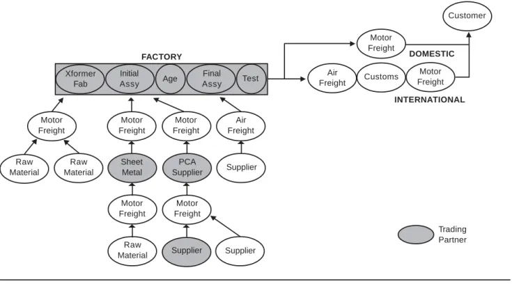
DEFINE THE SUPPLY CHAIN COMMUNITY The architecture of a supply chain is defined through the relationships of its trading partners. “A trading partner is an organization outside the firm that plays an integral role within the supply chain community, and whose financial fortune depends on the success of the supply chain community” [13]. In this supply chain the factory, the sheet metal supplier, the PCA sup-plier, and a custom semiconductor supplier were trading partners. The logistics service providers and most of the lower-level electronic parts suppliers, although essential to the product, were nominal trad-ing partners. This meant their financial success was largely independent of this particular supply chain. A nominal trading partner cannot be expected to par-ticipate in synchronized operations. Figure 1 dia-grams this supply chain and differentiates trading
Customer
PCA Supplier
FIGURE 1: Supply chain
partner nodes from nominal trading partner nodes. Unfortunately, the product design was old, and the individual product models took on their identity early in the upstream flow of the supply chain. If that were not the case, and the upstream flow was generic across the product family, it would have been a good opportu-nity to organize a downstream postponement opera-tion. One of the first components to be manufactured in the factory was the power transformer. The 14 product models required 11 different power transformers. Indi-vidual power transformers were then mounted onto one of three sheet metal chassis, and primary wiring was added. One of 4 front-panel subassemblies and 1 of 14 printed circuit assemblies were joined to the chassis in the factory at the initial assembly work center. At this point the product was turned on, and put into an aging rack to drive out any early component failures. Once the age process was successfully completed, the covers and a handle were added in final assembly. The prod-uct then completed an electrical safety test and final electrical performance tests in the factory before being packaged on the production line for shipment. When a product failed any of the testing, it was returned to a repair work center, then recycled through age and retested. In summary, a few raw materials became 11 transformers, 1 type of raw material plus hardware became 3 chassis,
Sheet Metal Raw Material Raw Material Motor Freight Motor Freight Motor Freight Air Freight Supplier Motor Freight Motor Freight Supplier Supplier Raw Material Air Freight Motor Freight Customs Motor Freight Xformer Fab Initial Assy Age Final Assy Test FACTORY INTERNATIONAL Trading Partner DOMESTIC
hundreds of purchased parts became 14 PCAs and, with a few additional purchased parts, became 14 products. DECIDE WHICH OF THE TRADING PARTNERS TO SYNCHRONIZE
Determining where to synchronize can be difficult. The reorder cycle time plus the manufacturing cycle time plus the outbound logistics transit time between inventory points in the supply chain must be compared against the customer order-to-delivery cycle time goal [12]. This is similar to, but different from, line balancing in a factory. The question to ask is, can the reorder be placed and the replenishment done reliably in the al-lotted time? In this supply chain the aging process was a natural inventory point. The head to shoulders tran-sition at the beginning of the PCA supplier’s process was a second natural inventory point. Table 2 analyzes the reorder-to-replenishment cycle time elements ver-sus the customer order-to-delivery goal.
The cycle time analysis shows that the trading part-ners to be included in the synchronization are the fac-tory (final assembly and test, initial assembly, and transformer fabrication), sheet metal fabricator, and PCA supplier. Notice that the inventory point at aging splits the factory into two different order-to-delivery loops. In addition, the factory aging process and initial assembly times are included as part of the total
TABLE 2: Supply Chain Cycle Time Analysis Customer order-to-delivery goal = SRT of 10 days
Supply Chain Path Cycle Time Remarks
1. Order + final assembly and test + transportation 10 days Okay to synchronize.
This sets the goal.
Factory Aging Process Inventory Point
2. Xformer + intial assembly reorder-to-replenishment Less than 10 days Okay to synchronize.
Includes the aging cycle time.
3. Sheet metal reorder-to-replenishment Less than 10 days Okay to synchronize.
Includes part of cycle time #2.
4. Galvanized sheet reorder-to-replenishment Less than 10 days Not synchronized. Nominal
trading partner. Use MRP.
5. PCA assembly reorder-to-replenishment Less than 10 days Okay to synchronize.
Includes part of cycle time #2.
6. Custom semiconductor reorder-to-replenishment More than 10 days Not synchronized.
Manage with MRP.
PCA Push/Pull Boundary Inventory Point
7. Purchased part reorder-to-replenishment More than 10 days Not synchronized. Cycle time
too long. Use MRP.
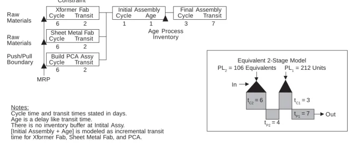
reorder-to-replenishment cycle times for transformer fabrication, sheet metal fabrication, and PCA assembly. The reason is that one transformer, one sheet metal chas-sis, and one printed circuit assembly flow together to become one product without any additional inventory buffering. Figure 2 shows how the synchronized por-tion of this supply chain can be represented by a two-stage supply chain model. The aging process can be viewed as a time delay in the flow, much like transit time. The custom semiconductor trading partner is cluded from synchronization because its cycle time ex-ceeds the required 10 days. The raw material distributor of galvanized sheet metal is also excluded from the syn-chronization because it is a nominal trading partner. SET THE CAPACITY FOR A CAPABLE SUPPLY CHAIN (THE DRUM)
In a synchronized supply chain every node, or trad-ing partner, that is included in the synchronized opera-tion must be capable. Capable means that the trading partner is willing to invest in sufficient capacity to meet the maximum daily throughput requirement [12]. The three factors used to determine capable capacity are the required customer service level, the minimum to maxi-mum range of daily production, and the potential to grow beyond the maximum range. The 14 products in this supply chain example varied from a mean of 5 units
FIGURE 2: Two-stage supply chain model System Constraint Raw Materials Raw Materials Push/Pull Boundary Age Process Inventory Notes:
Cycle time and transit times stated in days. Age is a delay like transit time.
There is no inventory buffer at Intital Assy.
[Initial Assembly + Age] is modeled as incremental transit time for Xformer Fab, Sheet Metal Fab, and PCA.
Xformer Fab
Cycle Transit
Sheet Metal Fab
Cycle Transit
Initial Assembly
Cycle Age
Final Assembly
Cycle Transit
Build PCA Assy
Cycle Transit MRP 6 6 6 2 2 2 1 1 3 7
Equivalent 2-Stage Model PL2 = 106 Equivalents PL1 = 212 Units In Out tC1 = 3 tP1 = 7 tP2 = 4 tC2 = 6
per month with a standard deviation of 11 units per month to a mean of 404 units per month with a stan-dard deviation of 219 units per month. When the his-torical market demand for all 14 products was combined statistically, the total mean was 1,524 units per month with a root mean squared (RMS) combined standard deviation of 374 units per month. It is valid to approxi-mate the combined standard deviation using an RMS calculation because the market demand for each prod-uct was independent of the market demand for the other products; there was little autocorrelation between prod-uct demands. Using an average of 21.5 work days per month, this supply chain needed to be capable of mixed-model production with a combined mean of 71 units per day and a combined RMS standard deviation of 17.4 units per day.
To achieve a 95% confidence level so that the target 10-day SRT could be maintained, each of the trading partners had to agree to a capable capacity investment equal to the mean plus two standard deviations of the historical market demand, or 106 units per day. This meant that 19 out of 20 days the supply chain would be able to deliver to a 10-day SRT no matter what the market demanded. There were four con-tenders for the system constraint: the capacity of the final test set, capacity of the aging process, capacity of a welding machine in magnetics fabrication, and capacity of the surface mount line at PCA assembly. It was determined by careful measurement that the welding machine in transformer fabrication was the
most constraining of the four; welding was the system constraint.
The minimum operating capacity is a second factor to consider in a synchronized operation. The rate of the market demand fluctuated day to day. One day a month, or 5% of the time, the demand for product would go as low as the mean minus two standard deviations or 36 units per day. That is only one-third of the maximum capacity for this line. It meant that culturally the workforce had to be willing and able to cross train, work on quality projects, or work for a day on another production line. Therefore, culturally, management had to understand that to achieve a 95% or higher service level some capacity would be idle part of the time. The return on investment of such capacity is driven by end-to-end supply chain throughput, not by machine utilization. It may be pru-dent for part of the workforce to be hired as temporary workers to add flexibility in managing capacity.
The probability of growth in market share is the third capacity consideration. The system constraint must be sized to achieve the customer service level while main-taining surge capacity at each of the other supply chain nodes. If the product line is expected to grow, by say 20% during the next year, then either today’s loading on the system constraint must be reduced by 20%, or 20% incremental capacity must be purchased and added to the system constraint in the necessary time frame. As the system constraint capacity is adjusted, a check must be made to ensure that the real system constraint has not shifted to another trading partner.
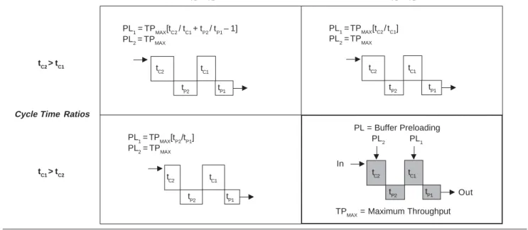
FIGURE 3: Calculating the buffer preloads for the two-stage supply chain PL = Buffer Preloading PL2 PL1 In Out tC2 tC1 tP1 tP2
TPMAX = Maximum Throughput PL1 = TPMAX[tC2/ tC1] PL2 = TPMAX tC2 tC1 tP1 tP2 PL1 = TPMAX[tC2/ tC1+ tP2/ tP1– 1] PL2 = TPMAX tC2 tC1 tP1 tP2 PL1 = TPMAX[tP2/tP1] PL2 = TPMAX tC2 tC1 tP1 tP2
tP2> tP1 Transit Time Ratios tP1> tP2
Cycle Time Ratios tC2> tC1
tC1> tC2
LEARN SYNCHRONIZED INVENTORY DYNAMICS (THE BUFFER)
Think of a synchronized supply chain as a sequence of trading partners arranged serially. The output of each upstream trading partner is connected by an outbound pipeline to the input of the next downstream trading partner. The last outbound pipeline connects directly with the end customer. Each stage of the supply chain network consists then of a trading partner node with its outbound pipeline. In a synchronized supply chain each node must be preloaded with inventory before operations can begin. This preload inventory makes each node capable of supporting the maximum through-put set by the system constraint. When the market de-mand is high, inventory transfers out of the node and into the pipeline. When market demand is low, inven-tory transfers out of the pipeline back into the node.
In the interest of not creating any more inventory than absolutely necessary, the quantity of inventory held in the aging process also functioned as the shipping buffer. This provided about two days of time buffer to solve any upstream issues, while still shipping on time. This was practical only when the process of final assembly and test had been shown to be predictable and reliable. Two different problems caused great variability in this portion of the line at start-up. The final test set would fail at random times, and the line would run out of packaging materials. Packaging was ordered weekly
by the MRP system. A second test set was built with duplicate capability and new protection circuitry that dramatically increased its uptime. And the test super-visor began ordering packaging direct from the sup-plier on the basis of the actual daily demand.
Likewise, the level of raw materials held in trans-former fabrication also functioned as the protective buffer for the welding machine, which was the system constraint. This was practical only after the winding, terminating, and stacking process between the raw material inventory and the welding machine had been shown to be predictable and reliable. Because this was not the case with a constantly changing transformer mix, two days of work-in-process inventory was com-pleted through the stacking operation and physically stored beside the welding machine. Of course, there was also purchased material inventory at the PCA supplier push/pull boundary, and there was raw material at the sheet metal fabricator.
The preload buffer inventory quantities are calculated from the equations presented in figure 3. A two-stage synchronized supply chain reference model is shown in the lower right portion of the figure. Each node has an associated cycle time and outbound pipeline transit time. The preload buffer inventory quantities for each node are calculated on the basis of the maximum throughput of the system constraint and the ratios of cycle times and pipeline transit times. The quadrant with the appropriate pair of equations is determined
on the basis of whether the cycle time for node2 is larger or smaller than for node1, and whether the transit time for node2 is larger or smaller than for node1. The equa-tions found in the upper-right quadrant were used for this example. The preload inventory for final assembly was 212 units at aging. The preload inventory for node2 included 106 transformers in magnetics fabrication, 106 chassis in sheet metal fabrication, and 106 printed cir-cuit assemblies at the PCA supplier. Once synchronized operations began, these quantities naturally split be-tween inventory at the node and inventory in the pipe-line.
BROADCAST THE CUSTOMER’S DEMAND (THE ROPE)
It is common knowledge that a long serial supply chain will exhibit the “bullwhip effect” [4, 7, 8]. That means the replenishment signal for a small change in customer demand becomes distorted and amplified as it propagates upstream toward the supplier. As a re-sult, the supplier is bullwhipped from periods of over-production to periods of no over-production. The bullwhip effect is caused by the combination of an upstream se-rial transmission of demand information between pairs of trading partners and a downstream delay in logis-tics transit time between pairs of trading partners. The bullwhip effect must be eliminated for a synchronized supply chain to be effective.
The proper way to minimize the bullwhip effect is to connect every trading partner in parallel to two demand signals. One demand signal, the actual demand, origi-nates from the point of sale at the customer. The second demand signal, the broadcast demand, originates from the system constraint. The actual demand signal is used to synchronize the shipping buffer with the system con-straint and with the rate of inbound materials flowing into the push/pull boundary. The broadcast demand is used to synchronize all the other pull trading part-ners [12]. In this supply chain the actual demand was routed in parallel to the aging process (shipping buffer), to the welding operation in transformer fabrication (sys-tem constraint), and to the PCA supplier’s materials planning system (push/pull boundary). The welding operation (system constraint) then forwarded the broad-cast demand in parallel to the first operation in final assembly, initial assembly, magnetics fabrication, sheet metal fabrication, and PCA assembly.
A set of daily operating rules determines the action to be taken by each of the trading partners downstream from the push/pull boundary. Should the system con-straint move to another trading partner, every trading
partner already has simultaneous access to both de-mand signals. Should the system constraint shift, an orderly changeover of system constraint roles and re-sponsibilities can take place.
Supply chain synchronization requires adherence to the following operational rules:
• “Rule 1: The customer end of the supply chain ships the actual demand rate and mix from its shipping buffer.
• Rule 2A: If the system constraint can meet the actual demand rate and mix, then it broadcasts the actual demand rate and mix as the broadcast demand. • Rule 2B: If the system constraint cannot meet the
ac-tual demand rate or mix, then it broadcasts a con-strained rate or mix as the broadcast demand, and it alone manages the customer order backlog, until throughput is caught up.
• Rule 3: Each day all other pull trading partners pro-duce the equivalent number of products or assem-blies required by the rate and mix of the broadcast demand.
• Rule 4: The push/pull boundary replenishes raw materials and purchased parts at the accumulated rate and mix of the actual demand” [11].
PLAN AT THE PUSH / PULL BOUNDARY
A pull system expects all the required material to be immediately available as needed. The buffer inventory that defines the push/pull boundary at the PCA sup-plier is replenished using the traditional production and inventory control methods of forecasting, sales and operations planning, master production scheduling (MPS), and MRP. It is essential that the rate and mix of market demand be forecast in units at least monthly. Forecast error is tracked against the rate and mix of the actual demand. In this supply chain raw materials and lower-level components for transformer fabrication, sheet metal fabrication, and PCA assembly were each replenished using MRP.
The push/pull boundary inventory at the PCA sup-plier contained component parts that were both com-mon across the 14 end products and unique to only one product. The part levels maintained in this inventory buffer were key to the supply chain’s ability to meet dynamic changes in product mix. When a part is com-mon, it requires less safety stock because of the risk-pooling effect [8]. Risk risk-pooling takes into account the statistical probability that with independently de-manded products an increase in demand of one prod-uct is likely to be counterbalanced by a decrease in demand of another product that uses the same part.
This looks like a smaller standard deviation in the part’s demand relative to the demand for a unique part. But when a part is unique, the standard deviation in that part’s demand appears to be larger relative to that of a common part. To guarantee a 95% service level, the part safety stock must be planned to cover the mean plus two standard deviations of the historical product de-mand times quantity usage per end product.
The MPS was managed to maximize the upside po-tential in a competitive, growing market. The plan for the first six weeks of the MPS was to build the maxi-mum throughput per day, or 530 units/week. The re-maining plan through the end of the MPS planning horizon was to build at a rate and mix equal to the mean of the historical data, or 355 units/week. Follow-ing rule 4, discussed above, actual daily orders were accumulated Monday through Friday of the current week. Every Friday the MPS plan for the following week was adjusted down to match the previous week’s ac-tual demand. And every Friday the sixth week’s plan was raised to the maximum throughput of 530 units/ week. By overdriving the front end of the MPS in this fashion, the planner could push out unnecessary pro-duction starts of PCAs, and the buyer could push out or cancel unnecessary purchases. Yet, the rate of incom-ing material would sustain the maximum throughput with 6 weeks of lead time for suppliers to react. The cost for this inventory shock absorber was 6 weeks x [530 units/week – 355 units/week] equaling 1,050 sets of lower-level parts. This was about 15 days supply of lower-level inventory on the basis of historical demand held by the PCA supplier.
KEEP THE SUPPLY CHAIN IN ALIGNMENT WITH EQUIVALENT THROUGHPUT AND TOTAL SYSTEM INVENTORY PERFORMANCE MEASURES
A pair of global performance measures, equivalent throughput and total system inventory, are used to keep the daily operations at each of the trading partners in alignment with the product line business strategy. These are global measures in that they serve to globally opti-mize the end-to-end supply chain, rather that just lo-cally optimizing the operations of one trading partner [10]. Go back for a moment to the idea of an idealized synchronized supply chain that has just one stockkeeping unit (SKU) moving through a series of downstream trading partners before reaching the end customer. Suppose that this SKU is not modified in any way as it is pulled downstream through the supply chain. If all the trading partners are in alignment, the
throughput of product entering each section of out-bound pipeline will be the same. And the sum of each trading partner’s node inventory and its outbound pipe-line inventory will be constant and equal to the preload inventory for each of the middle nodes. In fact, the total system inventory will be the number of nodes times the preload inventory. But if one of the trading partners begins to fall out of alignment, its throughput and re-sidual node inventory will deviate from the other trad-ing partners.
In the real world this idealized model must be ad-justed to account for three factors. First, not one SKU, but many SKUs, are being produced. Second, the prod-uct exists only as equivalent sets of lower-level parts, as one moves upstream toward the supplier. And third, different trading partners have different manufactur-ing cycle times and different outbound pipeline transit times. Some adjustments must be made to account for these differences.
“A synchronized supply chain is in alignment when the units per day of throughput for one trading partner, offset in time by that trading partner’s fixed cycle time, is equivalent to the units per day of throughput for each of the synchronized trading partners. This is the equiva-lent throughput performance measure.
• Throughput is measured in units entering the out-bound pipeline.
• Throughput at the trading partner node is offset by the amount of fixed cycle time in days that this node requires to convert an order into a shipment. • Throughput is independent of transit time.
• The bill of material defines the equivalency of part sets to the end product.
• Alignment is lost upstream from the push/pull boundary.” (Written by the author for the APICS Advanced Supply Chain Management (ASCM) courseware, © 2000 APICS.)
A supply chain is synchronized when…
the daily equivalent throughput at each node = the daily broadcast demand.
“A synchronized supply chain is in alignment when the units per day of inventory at one trading partner, adjusted for transit time ratios and cycle time ratios, is equivalent to the units per day of inventory for each of the synchronized trading partners. This is the Total Sys-tem Inventory performance measure.
• Inventory is measured in units remaining at the node and entering the pipeline.
• The most downstream node (closest to the customer) is the reference node.
• The preload inventory level for each synchronized trading partner is adjusted by the ratios of transit times and cycle times to the reference node.
• The bill of material defines the equivalency of part sets to the end product.
• Alignment is lost upstream from the push/pull boundary.” (Written by the author for the APICS ASCM courseware, © 2000 APICS.)
A supply chain is synchronized when… For the last supply chain stage1:
daily ending inventory1 [node + pipeline] = daily starting inventory1 [node + pipeline] + current broadcast demand – last broadcast demand.
For the next to last supply chain stage2:
daily equivalent end inventory2 = preload equivalent inventory2 – current broadcast demand.
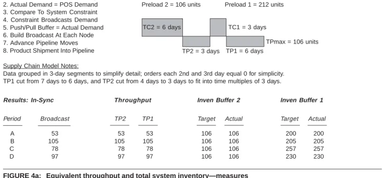
FIGURE 4a: Equivalent throughput and total system inventory—measures
Process Steps: Two-Stage Supply Chain Model:
1. Receive Inbound Into Inventory TC2 = Constraint
2. Actual Demand = POS Demand Preload 2 = 106 units Preload 1 = 212 units
3. Compare To System Constraint 4. Constraint Broadcasts Demand 5. Push/Pull Buffer = Actual Demand 6. Build Broadcast At Each Node 7. Advance Pipeline Moves 8. Product Shipment Into Pipeline Supply Chain Model Notes:
Data grouped in 3-day segments to simplify detail; orders each 2nd and 3rd day equal 0 for simplicity. TP1 cut from 7 days to 6 days, and TP2 cut from 4 days to 3 days to fit into time multiples of 3 days.
Results: In-Sync Throughput Inven Buffer 2 Inven Buffer 1
Period Broadcast TP2 TP1 Target Actual Target Actual
TC2 = 6 days TC1 = 3 days
TP2 = 3 days TP1 = 6 days
TPmax = 106 units
Figure 4 shows simulation results for this example and illustrates the dynamics of the daily equivalent throughput and total system inventory performance measures when the supply chain is synchronized. Fig-ure 4a details the model’s setup and resulting perfor-mance measures. Figure 4b shows simulated data for four periods at each node and in each pipeline. MANAGE THE DYNAMICS OF DEMAND RAMPING UP AND RAMPING DOWN
Over time the operating levels of any supply chain will change. Market conditions might improve or they might worsen. A particular product might suddenly become more popular and radically change the prod-uct mix. The key to managing such up and down dy-namics is the ability to know when the supply chain operating point falls outside the dynamic range for which it has been designed. Once a month the mean and RMS standard deviation are recomputed for the entire product family on the basis of the past six months of actual demand. The new month 6 demand data are added, and the old month 1 demand data are subtracted to arrive at a new six-month history. Product mix safety stock levels for each of the inventory buffers are recom-puted monthly using these revised historical demand data.
The supply chain capacity was designed to sustain
A B C D 53 105 78 97 53 105 78 97 53 105 78 97 106 106 106 106 200 205 257 230 106 106 106 106 200 205 257 230
a 95% service level over the range of the mean demand
+2 standard deviations of the demand. The supply
chain buffer inventory has been sized to sustain this maximum throughput rate over the six-month his-torical product mix. In a steadily rising market, in-cremental inventory must be added to each node and incremental capacity added to the system constraint before actual daily throughput can consistently ex-ceed the maximum throughput. Otherwise, the syn-chronization will be broken. Likewise, in a steadily falling market some inventory must be subtracted from each node and some capacity taken away from the system constraint to maintain a reasonable re-turn on inventory and capacity investments.
Once a month the past 20-day actual mean throughput is computed across all 14 product mod-els. This is checked against upper and lower control limits with an eye on the sales forecast. As the 20-day actual mean throughput approaches either con-trol limit, the operating design of the synchronized supply chain must change. The control limits should take into account both underlying trends in the ac-tual demand and the calendar time it will take to implement the required changes to capacity and in-ventory. On the one hand these triggers should not cause volatility in planning capacity and inventory, but on the other hand they should catch significant upward and downward trends in time to adjust capacity and inventory.
Upper control limit = trigger to buy some node capacity and inventory
Upper control limit = mean capacity + 25% = 89 average units/day
Lower control limit = trigger to sell some node capacity and inventory
Lower control limit = mean capacity – 25% = 53 average units/day
SUMMARY
This case study presented a detailed description of the synchronization of the final two stages of an international supply chain for an electronics instru-mentation manufacturer. The product line was trans-formed from a traditional MRP-driven build-to-stock manufacturing operation into a build-to-order syn-chronized supply chain. That transformation suc-cessfully reduced the supplier response time from an inconsistent 3–5 weeks to a consistent 10 days across all products. The practical application of Eli Goldratt’s drum-buffer-rope TOC concepts to syn-chronize the supply chain resulted in excellent de-livery performance for a medium investment in capacity, inventory, and information management. The supply chain redesign objective was accom-plished, and synchronization was sustained dur-ing many months of volatile demand.
FIGURE 4b: Equivalent throughput and total system inventory—simulation
Days Demand Broadcast Push/Pull Buffer Stage 2 Stage 1 Delivery
Starting Condition 48 58 0 48 104 48 60
Node + Pipeline Inventory 106 212
A: 1–> 3 53 + 0 + 0 53
53 53 0 53 99 53 48 Prior
Throughput 53 53 Demand
Node + Pipeline Inventory 106 + 53 – 53 = 106 212 + 48 – 60 = 200 0 + 0 + 60
B: 4–> 6 105 + 0 + 0 105
105 1 0 105 47 105 53 Prior
Throughput 105 105 Demand
Node + Pipeline Inventory 106 + 105 – 105 = 106 200 + 53 – 48 = 205 0 + 0 + 48
C: 7–> 9 78 + 0 + 0 78
78 28 0 78 74 78 105
Throughput 78 78
Node + Pipeline Inventory 106 + 78 – 78 = 106 205 + 105 – 53 = 257 0 + 0 + 53
D: 10 –> 12 97 + 0 + 0 97
97 9 0 97 55 97 78
Throughput 97 97
The following is a summary of the practical lessons learned from this case:
• Drum: Define capacity in daily equivalent units. Use historical statistical demand information to determine the capacity required by each node to maintain a 95% service level. The capacity investment was described in terms of every trading partner being capable of the maximum daily throughput. This means some ex-cess capacity at most trading partner sites and the need to maintain a flexible workforce. The process downstream from the system constraint must be to-tally reliable. Be prepared to adjust the constraint capacity up or down as the average rate of actual demand shifts.
• Buffer: Define inventory in daily equivalent units. Equations to calculate the levels of buffer preload inventory were presented for a two-stage synchro-nized supply chain. The inventory investment was described in terms of preload inventory plus safety stock held at the push/pull boundary plus inven-tory risk pools for unique materials at the point of consumption. Overdrive the front end of the MPS to maintain the upside potential for throughput, and adjust node inventory up or down as the average rate of actual demand shifts.
• Rope: Pull to customer demand. Broadcast demand daily throughout the supply chain in a way that eliminates serial communications and delay, thereby defeating the bullwhip effect. Let the system con-straint trading partner manage order backlog. • Performance measures: A new description of equivalent
throughput and total system inventory as two global performance measures was presented as a primary means of keeping a synchronized supply chain in alignment.
REFERENCES
1. Alber, K.L., and W.T. Walker. Supply Chain Management Prin-ciples and Techniques for the Practitioner. Falls Church, Va.: APICS Educational and Research Foundation, 1998.
2. Covington, J.W. Tough Fabric: The Domestic Apparel and Textile Chain Regains Market Share. Severna Park, Md.: Chesapeake Consulting, 1996.
3. Goldratt, E.M., and J. Cox. The Goal: Excellence In Manufactur-ing. Croton-on-Hudson, N.Y.: North River Press, 1984. 4. Lee, H.L., V. Padmanabhan, and S. Whang, “The Bullwhip
Effect in Supply Chains.” Sloan Management Review (spring 1997): 93–102.
5. Noreen, E., D. Smith, and J.T. Mackey. The Theory of Con-straints and its Implications for Management Accounting. Great Barrington, Mass.: North River Press, 1995.
6. Schragenheim, E., and H.W. Dettmer. Manufacturing at Warp Speed: Optimizing Supply Chain Financial Performance.
Boca Raton, Fla.: St. Lucie Press, 2001.
7. Senge, P.M. The Fifth Discipline: The Art and Practice of the Learning Organization. N.Y.: Doubleday/Currency, 1990. 8. Simchi-Levi, D., P. Kaminsky, and E. Simchi-Levi. Designing
and Managing the Supply Chain. Boston, Mass.: Irwin McGraw-Hill, 2000.
9. Smith, D. The Measurement Nightmare: How the Theory of Con-straints Can Resolve Conflicting Strategies, Policies, and Measures. Boca Raton, Fla.: St. Lucie Press, 2000.
10. Walker, W.T. “Defining Supply Chain Management.” 1999 APICS Educational and Research Foundation Summer Academic/ Practitioner Workshop Proceedings. Alexandria, Va.: APICS Edu-cational & Research Foundation, 1999, 115–120.
11. Walker, W.T. “Synchronized for Growth.” APICS The Perfor-mance Advantage (April 2001): 26–29.
12. Walker, W.T. “Synchronizing Supply Chain Operations.” 2000 APICS International Conference Proceedings. Alexandria, Va.: APICS, 2000, 8–15.
13. Walker, W.T. and K.L. Alber. “Understanding Supply Chain Management.”APICS—The Performance Advantage (January 1999): 38–43.
About the Author—
WILLIAM T. WALKER, CFPIM, CIRM, is a Sup-ply Chain Architect. He spent over 30 years work-ing both sides of the interface between supply chain management and new product development for Hewlett-Packard, now Agilent Technologies. He is accomplished in developing and optimizing inter-national supply chains, has firsthand experience in worldwide product transfer logistics, and has personally developed successful new products. He is a Logistics Forum 2000 “Top 20 Logistics Ex-ecutive” award winner. Mr. Walker co-developed the principles of supply chain management taught by APICS and is a co-author of the book Supply Chain Management: Principles and Techniques for the Practitioner. Mr. Walker is a past president of the APICS Educational and Research Foundation, where he collaborated on setting education strategy; and a past APICS Vice President of Education-Specific Industry Groups, where he had oversight responsibility for education de-veloped for Aerospace and Defense, Process In-dustry, Repetitive, Remanufacturing, Small Manufacturing, and Textile/Apparel SIGs. He is APICS certified at the Fellow level, and holds BSEE and MSIE degrees from Lehigh University. He can be reached at [email protected].