B-spline neural network based digital baseband predistorter
solution using the inverse of De Boor algorithm
Xia Hong, Yu Gong and Sheng Chen
Abstract— In this paper a new nonlinear digital baseband predistorter design is introduced based on direct learning, together with a new Wiener system modeling approach for the high power amplifiers (HPA) based on the B-spline neural network. The contribution is twofold. Firstly, by assuming that the nonlinearity in the HPA is mainly dependent on the input signal amplitude the complex valued nonlinear static function is represented by two real valued B-spline neural networks, one for the amplitude distortion and another for the phase shift. The Gauss-Newton algorithm is applied for the parameter estimation, in which the De Boor recursion is employed to calculate both the B-spline curve and the first order derivatives. Secondly, we derive the predistorter algorithm calculating the inverse of the complex valued nonlinear static function according to B-spline neural network based Wiener models. The inverse of the amplitude and phase shift distortion are then computed and compensated using the identified phase shift model. Numerical examples have been employed to demonstrate the efficacy of the proposed approaches.
I. INTRODUCTION
The operation of high power amplifiers (HPA) in modern wireless communication systems introduces serious nonlin-earities, potentially leading to the deterioration in system performance. The digital baseband predistorter is a functional device precedes the HPA. It acts as the inverse function of the HPA and predistorts the HPA input signal. The modeling of high power amplifiers (HPA) is crucial in any linearisation techniques of broadband communication systems employing power-efficient nonlinear HPA transmitter [1], [2]. Various HPA models and the associated predistorter (PD) design have been researched [3], [4], [5], [6]. The available digital baseband PD can be classified as indirect learning or direct learning. The indirect learning approaches are realised by initially identifying a post-inverse filter for the HPA followed by copying it into the PD [7], [8], [9]. The direct learning PD is obtained by initially identifying the input-output relation of the HPA, followed by designing the PD based on the identified HPA model [10], [11], [2], [12]. The indirect learning PD is simpler to implement but it may suffer from modelling bias due to error propagation from noise, thus the deterioration in performance. Thus it is highly desirable to develop highly efficient PD approaches based on direct learning.
The Wiener model has been used as a model for some industrial/biological systems [13], [14], [15], [16], and no-tably the HPA in broadband communication transmitters [17]. Xia Hong and Yu Gong are with School of Systems Engineering, University of Reading,UK (email: [email protected]), Sheng Chen is with School of Electronics and Computer Science, University of Southamp-ton,UK
Various approaches have been developed [18], [19], [20], [14], [21]. The model characterization/representation of the unknown nonlinear static function in the Wiener model is fundamental to its identification, control and/or other signal processing applications. Based on the approximation theory, the polynomial functions are appropriate in approximating the unknown nonlinear static functions. The B-spline curves consist of many polynomial pieces, offering versatility. The early work on the construction of B-spline curve is math-ematically involved and numerically unstable [22]. The De Boor algorithm uses recurrence relations and is numerically stable [22]. The B-spline basis functions for nonlinear sys-tems modelling have been widely applied [23].
In this work a new digital baseband predistorter solution is introduced based on direct learning. We initially consider HPA as complex valued Wiener system. Without losing generality it is assumed that the nonlinearity in the Wiener model is mainly dependent on the input signal amplitude. Consequently the complex valued nonlinear static function is represented by two real valued B-spline neural networks, one for the amplitude distortion and another for the phase shift, respectively. By minimizing the mean square error (MSE) between the model output and the system output, the Gauss-Newton algorithm is readily applicable for the parameter estimation in the proposed model. The Gauss-Newton algorithm is applied, which incorporates with the De Boor algorithm, including both the B-spline curve and the first order derivatives recursion. The proposed model based on B-spline functions is advantageous as this offers modeling versatility as well as enables stable and efficient evaluations of functional and derivative values, as required in nonlinear optimization algorithm. The Wiener model for memory HPAs is described in Section II, followed by the proposed new B-spline Wiener system modeling approach that is introduced in Section III.
Because the predistorter acts as the inverse function of the HPA and predistorts the HPA input signal, clearly the resultant PD is a Hammerstein model that is the inverse of the complex valued nonlinear static function, followed by the inverse of the linearity filter in the Wiener system. In Section IV a new PD design is introduced, including the efficient algorithm to calculate the inverse of the nonlinear static func-tion based on the proposed Wiener models. The inverse of the amplitude distortion is computed using the Newton-Raphson formula combining with De Boor algorithms, referred as the inverse of De Boor algorithm, followed by the calculation of the phase distortion using the identified phase shift model. Numerical examples have been employed to demonstrate the
efficacy of the proposed approaches.
II. THEWIENER MODEL FOR MEMORYHPAS The general complex valued Wiener system consists of a cascade of two subsystems, a linear filter of order 𝑛 representing the memory effect on the input signal as the first subsystem, followed by a nonlinear memoryless function Ψ(∙) :𝒞 → 𝒞 as the second subsystem. The system can be represented by
𝑤(𝑡) = 𝐻(𝑧)𝑦(𝑡)
= 𝑦(𝑡) +ℎ1𝑦(𝑡−1)...+ℎ𝑛𝑦(𝑡−𝑛) (1)
𝑑(𝑡) = Ψ (𝑤(𝑡)) +𝜉(𝑡) (2) with𝑧 transfer function𝐻(𝑧)defined by
𝐻(𝑧) =∑𝑛 𝑖=0
ℎ𝑖𝑧−𝑖, ℎ0= 1 (3)
where 𝑑(𝑡) = 𝑑𝑅(𝑡) +𝑗⋅𝑑𝐼(𝑡) ∈ 𝒞 is the system output and 𝑦(𝑡) = 𝑦𝑅(𝑡) +𝑗 ⋅𝑦𝐼(𝑡) ∈ 𝒞 is the system input.
𝑗 = √−1. 𝜉(𝑡) = 𝜉𝑅(𝑡) +𝑗𝜉𝐼(𝑡) ∈ 𝒞 is assumed to be a white complex valued noise sequence independent of𝑦(𝑡). Both𝜉𝑅(𝑡)and𝜉𝐼(𝑡)are zero mean and have a variance of
𝜎2. 𝑤(𝑡) = 𝑤
𝑅(𝑡) +𝑗 ⋅𝑤𝐼(𝑡) ∈ 𝒞 is the output of linear filter subsystem and the input to the nonlinear subsystem.
ℎ𝑖 = ℎ𝑖,𝑅 +𝑗 ⋅ℎ𝑖,𝐼, (𝑖 = 1,⋅ ⋅ ⋅ , 𝑛) are complex valued coefficients of the linear filter.𝑛is assumed known. Denote h= [ℎ1, ..., ℎ𝑛]𝑇 ∈ 𝒞𝑛.
For the baseband HPA model, Ψ (𝑤(𝑡))can be specified by a nonlinearity of the traveling wave tube (TWT) [17]. The input to the TWT nonlinearity can be expressed as
𝑤(𝑡) =∣𝑤(𝑡)∣exp(𝑗∠𝑤(𝑡)) =𝑟(𝑡) exp(𝑗⋅𝜙(𝑡)) (4) where 𝑟(𝑡) = √𝑤2𝑅(𝑡) +𝑤2𝐼(𝑡) and 𝜙(𝑡) = arctan(𝑤𝐼(𝑡)/𝑤𝑅(𝑡)), denoting the amplitude and phase of
𝑤(𝑡)respectively. The output of TWT,Ψ (𝑤(𝑡)), is distorted in both the amplitude and the phase, with the distortion dependent mainly on the input signal amplitude, i.e. 𝑟(𝑡). SoΨ (𝑤(𝑡))can be expressed by [17]
Ψ (𝑤(𝑡)) = ∣Ψ (𝑤(𝑡))∣exp(𝑗⋅∠Ψ (𝑤(𝑡))) = 𝑟Ψ(𝑡) exp(𝑗⋅[𝜙Ψ(𝑡) +𝜙(𝑡)]) (5) where𝑟Ψ(𝑡)and𝜙Ψ(𝑡)denote the amplitude and phase shift byΨ (𝑤(𝑡))respectively, and these are given by
𝑟Ψ(𝑡) = { 𝛼1𝑟(𝑡) 1+𝛼2𝑟2(𝑡), 0≤𝑟(𝑡)≤𝑟𝑆𝑎𝑡 Ψ𝑚𝑎𝑥, 𝑟(𝑡)> 𝑟𝑆𝑎𝑡 (6) 𝜙Ψ(𝑡) = 𝛽1𝑟 2(𝑡) 1 +𝛽2𝑟2(𝑡). (7)
where 𝛼1, 𝛼2, 𝛽1, 𝛽2 are unknown parameters. 𝑟𝑆𝑎𝑡=
√
1 𝛼2 and Ψ𝑚𝑎𝑥 = 𝛼1
2√𝛼1. Our aim is the system identification for the above HPA model, i.e. given an observational in-put/output data set 𝐷𝑁 = {𝑦(𝑡), 𝑑(𝑡)}𝐾𝑡=1, to identify the underlying nonlinear function Ψ(∙) and to estimate the parametersℎ𝑖’s of the linear filter simultaneously. Note that
the signal𝑤(𝑡)between the two subsystems are unavailable. In this work we propose to model Ψ(∙) by using B-spline curves. Specifically, 𝑟Ψ(𝑡) and 𝜙Ψ(𝑡) are modeled by two univariate B-spline networks (B-spline curves) respectively as described in the following.
III. THE SYSTEM IDENTIFICATION ALGORITHM
A. Modelling ofΨ(∙)using B-spline function approximation Univariate B-spline basis functions are parameterized by the order of a piecewise polynomial of order𝑘, and also by a knot vector which is a set of values defined on the real line that break it up into a number of intervals. Supposing that there are𝑑basis functions, the knot vector is specified by(𝑀+𝑘)knot values,{𝑅1, 𝑅2,⋅ ⋅ ⋅, 𝑅𝑀+𝑘}. At each end there are 𝑘 knots satisfying the condition of being external to the input region, and as a result the number of internal knots is(𝑀−𝑘). Specifically
𝑅1< 𝑅2< 𝑅𝑘=𝑅𝑚𝑖𝑛< 𝑅𝑘+1< 𝑅𝑘+2< ⋅ ⋅ ⋅< 𝑅𝑀 < 𝑅𝑚𝑎𝑥=𝑅𝑀+1<⋅ ⋅ ⋅< 𝑅𝑀+𝑘. (8) Given these predetermined knots, a set of𝑀 B-spline basis functions can be formed by using the De Boor recursion [22], given by ℬ(0)𝑙 (𝑟) = { 1 if𝑅𝑙≤𝑟 < 𝑅𝑙+1 0 otherwise (9) 𝑙= 1,⋅ ⋅ ⋅,(𝑀 +𝑘) ℬ(𝑙𝑖)(𝑟) = 𝑟−𝑅𝑙 𝑅𝑖+𝑙−𝑅𝑙ℬ (𝑖−1) 𝑙 (𝑟) + 𝑅𝑖+𝑙+1−𝑟 𝑅𝑖+𝑙+1−𝑅𝑙+1ℬ (𝑖−1) 𝑙+1 (𝑟), 𝑙= 1,⋅ ⋅ ⋅,(𝑀+𝑘−𝑖) ⎫ ⎬ ⎭ 𝑖= 1,⋅ ⋅ ⋅, 𝑘 (10)
The derivative of B-spline basis function ℬ𝑙(𝑘)(𝑟) can be readily computed as 𝑑 𝑑𝑟[ℬ𝑙(𝑘)(𝑟)] = 𝑅 𝑘 𝑘+𝑙−𝑅𝑙ℬ (𝑘−1) 𝑙 (𝑟) −𝑅 𝑘 𝑘+𝑙+1−𝑅𝑙+1ℬ (𝑘−1) 𝑙+1 (𝑟) 𝑙= 1,⋅ ⋅ ⋅, 𝑀 (11) We model Ψ(∙) as two univariate B-spline neural net-works [23], one for the amplitude and another for the phase shift, in the form of
𝑟Ψ(𝑡) = 𝑀 ∑ 𝑙=1 ℬ𝑙(𝑘)(𝑟(𝑡))𝜔𝑙 (12) 𝜙Ψ(𝑡) = 𝑀 ∑ 𝑙=1 ℬ𝑙(𝑘)(𝑟(𝑡))𝜗𝑙 (13) and their derivatives are in the form of
𝑟′ Ψ(𝑡) = 𝑀 ∑ 𝑙=1 𝑑 𝑑𝑟(𝑡)ℬ𝑙(𝑘)(𝑟(𝑡))𝜔𝑙 (14) 𝜙′ Ψ(𝑡) = 𝑀 ∑ 𝑙=1 𝑑 𝑑𝑟(𝑡)ℬ𝑙(𝑘)(𝑟(𝑡))𝜗𝑙 (15)
where 𝜔𝑙’s and 𝜗𝑙’s are weights to be determined. Denote
𝝎 = [𝜔1,⋅ ⋅ ⋅, 𝜔𝑀]𝑇 ∈ ℜ𝑀 and 𝝑 = [𝜗1,⋅ ⋅ ⋅, 𝜗𝑀]𝑇 ∈ ℜ𝑀. Note that due to the piecewise nature of B-spline functions, there are only(𝑘+1)basis functions with nonzero functional/derivative values at any point 𝑟. Hence the com-putational cost of the De Boor algorithm is determined by the polynomial order𝑘, rather than the number of knots, and this is in the order of𝑂(𝑘2).
B. The main algorithm
The complex valued B-spline network output is denoted by𝑑ˆ(𝑡) = ˆ𝑑𝑅(𝑡) +𝑗⋅𝑑ˆ𝐼(𝑡)in which
ˆ
𝑑𝑅(𝑡) = 𝑟Ψ(𝑡) cos[𝜙Ψ(𝑡) +𝜙(𝑡)] ˆ
𝑑𝐼(𝑡) = 𝑟Ψ(𝑡) sin[𝜙Ψ(𝑡) +𝜙(𝑡)]
Let the error between the Wiener system output𝑑(𝑡)and the B-spline network output 𝑑ˆ(𝑡)be denoted by 𝑒(𝑡) = 𝑑(𝑡)−
ˆ
𝑑(𝑡) =𝑒𝑅(𝑡) +𝑗⋅𝑒𝐼(𝑡)∈ 𝒞. Our task is to estimate h, 𝝎 and𝝑. This could be achieved by minimizing
𝐽 = 𝐾 ∑ 𝑡=1 [𝑒𝑅(𝑡)]2+∑𝐾 𝑡=1 [𝑒𝐼(𝑡)]2 (16) Denote 𝝐 = [𝜖1, 𝜖2,⋅ ⋅ ⋅, 𝜖2𝐾]𝑇 = [𝑒𝑅(1),⋅ ⋅ ⋅, 𝑒𝑅(𝐾), 𝑒𝐼(1),⋅ ⋅ ⋅, 𝑒𝐼(𝐾)]𝑇 ∈ ℜ2𝐾, 𝜽 = [𝜃1 , 𝜃2, ⋅ ⋅ ⋅, 𝜃2(𝑑+𝑛)]𝑇 = [𝜔1, 𝜔2,⋅ ⋅ ⋅ , 𝜔𝑀, 𝜗1, 𝜗2,⋅ ⋅ ⋅, 𝜗𝑀, ℎ1,𝑅, ⋅ ⋅ ⋅ , ℎ𝑛,𝑅, ℎ1,𝐼, ⋅ ⋅ ⋅ , ℎ𝑛,𝐼]𝑇 ∈ ℜ2(𝑀+𝑛). Note that from (1) { 𝑤𝑅(𝑡) = 𝑦𝑅(𝑡) +∑𝑛𝑖=1(ℎ𝑖,𝑅𝑦𝑅(𝑡−𝑖)−ℎ𝑖,𝐼𝑦𝐼(𝑡−𝑖)) 𝑤𝐼(𝑡) = 𝑦𝐼(𝑡) +∑𝑛𝑖=1(ℎ𝑖,𝐼𝑦𝑅(𝑡−𝑖) +ℎ𝑖,𝑅𝑦𝐼(𝑡−𝑖)) (17) and for𝑖= 1,⋅ ⋅ ⋅, 𝑛, we have
⎧ ⎨ ⎩ ∂𝑤𝑅(𝑡) ∂ℎ𝑖,𝑅 = 𝑦𝑅(𝑡−𝑖) ∂𝑤𝑅(𝑡) ∂ℎ𝑖,𝐼 = −𝑦𝐼(𝑡−𝑖) ∂𝑤𝐼(𝑡) ∂ℎ𝑖,𝑅 = 𝑦𝐼(𝑡−𝑖) ∂𝑤𝐼(𝑡) ∂ℎ𝑖,𝐼 = 𝑦𝑅(𝑡−𝑖) (18)
Thus it can be shown that
{ ∂𝑟(𝑡) ∂ℎ𝑖,𝑅 = 1 𝑟(𝑡)[𝑤𝑅(𝑡)𝑦𝑅(𝑡−𝑖) +𝑤𝐼(𝑡)𝑦𝐼(𝑡−𝑖)] ∂𝑟(𝑡) ∂ℎ𝑖,𝐼 = 1 𝑟(𝑡)[𝑤𝐼(𝑡)𝑦𝑅(𝑡−𝑖)−𝑤𝑅(𝑡)𝑦𝐼(𝑡−𝑖)] (19) and { ∂𝜙(𝑡) ∂ℎ𝑖,𝑅 = 1 𝑟2(𝑡)[𝑤𝑅(𝑡)𝑦𝐼(𝑡−𝑖)−𝑤𝐼(𝑡)𝑦𝑅(𝑡−𝑖)] ∂𝜙(𝑡) ∂ℎ𝑖,𝐼 = 1 𝑟2(𝑡)[𝑤𝑅(𝑡)𝑦𝑅(𝑡−𝑖) +𝑤𝐼(𝑡)𝑦𝐼(𝑡−𝑖)] (20) We denote an iteration step variable by a superscript(𝜏), and apply the Gauss Newton algorithm as follows.
The Gauss Newton algorithm combined with the De Boor algorithm: With an initial𝜽(0), the iteration formula is given by
𝜽(𝜏)=𝜽(𝜏−1)−𝛼{[J(𝜏)]𝑇J(𝜏)}−1[J(𝜏)]𝑇𝝐(𝜽(𝜏−1)) (21)
where 𝛼 > 0 is a small positive step size. J denotes the Jacobian of 𝝐(𝜽) and is given by J = {∂𝜖∂𝜃𝑝
𝑞}, where for 𝑝= 1,⋅ ⋅ ⋅, 𝐾, and𝑡=𝑝. ∂𝜖𝑝 ∂𝜃𝑞 = ⎧ ⎨ ⎩ ∂𝑒𝑅(𝑡) ∂𝜔𝑙 =−ℬ (𝑘) 𝑙 (𝑟(𝑡)) cos[𝜙Ψ(𝑡) +𝜙(𝑡)], for 𝑞= 1,⋅ ⋅ ⋅ , 𝑀, (𝑙=𝑞) ∂𝑒𝑅(𝑡) ∂𝜗𝑙 =𝑟Ψ(𝑡) sin[𝜙Ψ(𝑡) +𝜙(𝑡)]ℬ (𝑘) 𝑙 (𝑟(𝑡)), for 𝑞=𝑀+ 1,⋅ ⋅ ⋅ ,2𝑀, (𝑙=𝑞−𝑀) ∂𝑒𝑅(𝑡) ∂ℎ𝑖,𝑅 =− {𝑟 ′ Ψ(𝑡) cos[𝜙Ψ(𝑡) +𝜙(𝑡)] −𝑟Ψ(𝑡) sin[𝜙Ψ(𝑡) +𝜙(𝑡)]𝜙′Ψ(𝑡)}∂ℎ∂𝑟(𝑖,𝑅𝑡) +𝑟Ψ(𝑡) sin[𝜙Ψ(𝑡) +𝜙(𝑡)]∂ℎ∂𝜙𝑖,𝑅(𝑡), for 𝑞= 2𝑀 + 1,⋅ ⋅ ⋅,2𝑀+𝑛, (𝑖=𝑞−2𝑀) ∂𝑒𝑅(𝑡) ∂ℎ𝑖,𝐼 =− {𝑟 ′ Ψ(𝑡) cos[𝜙Ψ(𝑡) +𝜙(𝑡)] −𝑟Ψ(𝑡) sin[𝜙Ψ(𝑡) +𝜙(𝑡)]𝜙′Ψ(𝑡)}∂𝑟∂ℎ(𝑖,𝐼𝑡) +𝑟Ψ(𝑡) sin[𝜙Ψ(𝑡) +𝜙(𝑡)]∂𝜙∂ℎ(𝑖,𝐼𝑡), for 𝑞= 2𝑀 +𝑛+ 1,⋅ ⋅ ⋅,2(𝑀 +𝑛), (𝑖=𝑞−2𝑀 −𝑛) (22) and for 𝑝=𝐾+ 1,⋅ ⋅ ⋅ ,2𝐾, and𝑡= (𝑝−𝐾)
∂𝜖𝑝 ∂𝜃𝑞 = ⎧ ⎨ ⎩ ∂𝑒𝐼(𝑡) ∂𝜔𝑙 =−ℬ (𝑘) 𝑙 (𝑟(𝑡)) sin[𝜙Ψ(𝑡) +𝜙(𝑡)], for 𝑞= 1,⋅ ⋅ ⋅ , 𝑀, (𝑙=𝑞) ∂𝑒𝐼(𝑡) ∂𝜗𝑙 =−𝑟Ψ(𝑡) cos[𝜙Ψ(𝑡) +𝜙(𝑡)]ℬ (𝑘) 𝑙 (𝑟(𝑡)), for 𝑞=𝑀+ 1,⋅ ⋅ ⋅ ,2𝑀, (𝑙=𝑞−𝑀) ∂𝑒𝐼(𝑡) ∂ℎ𝑖,𝑅 =− {𝑟′Ψ(𝑡) sin[𝜙Ψ(𝑡) +𝜙(𝑡)] +𝑟Ψ(𝑡) cos[𝜙Ψ(𝑡) +𝜙(𝑡)]𝜙′Ψ(𝑡)}∂ℎ∂𝑟(𝑖,𝑅𝑡) −𝑟Ψ(𝑡) cos[𝜙Ψ(𝑡) +𝜙(𝑡)]∂ℎ∂𝜙𝑖,𝑅(𝑡), for 𝑞= 2𝑀 + 1,⋅ ⋅ ⋅,2𝑀+𝑛, (𝑖=𝑞−2𝑀) ∂𝑒𝐼(𝑡) ∂ℎ𝑖,𝐼 =− {𝑟 ′ Ψ(𝑡) sin[𝜙Ψ(𝑡) +𝜙(𝑡)] +𝑟Ψ(𝑡) cos[𝜙Ψ(𝑡) +𝜙(𝑡)]𝜙′Ψ(𝑡)}∂𝑟∂ℎ(𝑖,𝐼𝑡) −𝑟Ψ(𝑡) cos[𝜙Ψ(𝑡) +𝜙(𝑡)]∂𝜙∂ℎ(𝑖,𝐼𝑡) for 𝑞= 2𝑀 +𝑛+ 1,⋅ ⋅ ⋅ ,2(𝑀+𝑛) (𝑖=𝑞−2𝑀−𝑛) (23) Note that we propose that the De Boor algorithm (9)-(11) are utilized for evaluating (12)-(15), which are then applied in evaluating the entries for (22)-(23). In addition (19)-(20) are also used to calculating the entries for (22)-(23). The iterative equation (21) can be terminated when 𝜽(𝜏) converges, or by predetermining a sufficiently large number of iterations. Using the final model parameters it is straightforward to produce estimated value of ˆ𝑟𝑆𝑎𝑡 and ˆΨ𝑚𝑎𝑥using numerical search that will then be used in PD design in Section IV.
As the objective function of (16) is highly nonlinear, the solution of Gauss Newton algorithm is dependent on the initial condition. It is important that 𝜽(0) is properly initialized so that it is as closer as possible to optimal solution, and it is also desirable the parameter initialization is simple to implement.
C. A simple parameter initialization using least squares algorithm
Initially a set of (𝑀 +𝑘) knot vector is predetermined that breaks the domain of 𝑟(𝑡) up, with𝑘 knots satisfying the condition of being external to the regions for𝑟(𝑡)at each end. In this work, the parameter𝜽(0)is initialized as follows. 1) Initialize ℎ(0)𝑖 = 0, i.e. ℎ(0)𝑖,𝑅 = 0, ℎ(0)𝑖,𝐼 = 0, for 𝑖 =
1, ..., 𝑛.
2) Generate a sequence 𝑟(0)(𝑡) = √𝑦2𝑅(𝑡) +𝑦𝐼2(𝑡), for
𝑡= 1, ..., 𝐾.
3) Generate a sequence 𝑟(0)𝑑 (𝑡) = √𝑑𝑅2(𝑡) +𝑑2𝐼(𝑡), for
𝑡= 1, ..., 𝐾. Denoter𝑑= [𝑟𝑑(0)(1), ..., 𝑟(0)𝑑 (𝐾)]𝑇. 4) Generate a sequence 𝜙(0)Ψ (𝑡) = arctan(𝑑𝑑𝐼(𝑡)
𝑅(𝑡)) −
arctan(𝑦𝐼(𝑡)
𝑦𝑅(𝑡)), and then limit the values within [
𝜋 2,𝜋2] as appropriate (by adding a multiple of ±2𝜋 if out of range), for 𝑡 = 1, ..., 𝐾. Denote 𝝓Ψ = [𝜙(0)Ψ (1), ..., 𝜙(0)Ψ (𝐾)]𝑇.
5) Form a regression matrix
B= ⎡ ⎢ ⎢ ⎢ ⎢ ⎢ ⎢ ⎢ ⎢ ⎣ ℬ(𝑘) 1 (𝑟(0)(1)) ⋅ ⋅ ⋅ ℬ𝑀(𝑘)(𝑟(0)(1)) .. . . .. ... .. . ℬ(𝑘)𝑙 (𝑟(0)(𝑡)) ... .. . . .. ... ℬ(𝑘)1 (𝑟(0)(𝐾)) ⋅ ⋅ ⋅ ℬ𝑀(𝑘)(𝑟(0)(𝐾)) ⎤ ⎥ ⎥ ⎥ ⎥ ⎥ ⎥ ⎥ ⎥ ⎦ ∈ ℜ𝐾×𝑀 (24)
6) Compute the least square estimate 𝝎(0) = (B𝑇B)−1B𝑇r𝑑, and𝝑(0)= (B𝑇B)−1B𝑇𝝓
Ψ. 7) Finally set𝜽(0)= [0 , ...,0
2𝑛
, [𝝎(0)]𝑇, [𝝑(0)]𝑇]𝑇. IV. NEW PREDISTORTER SOLUTION USING THE INVERSE
OFDEBOOR ALGORITHM
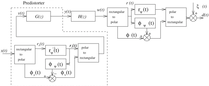
In Section III, the models of the amplitude distortion and the phase shift of the HPA have been constructed as two univariate B-spline curves respectively. The proposed PD to the Wiener HPA, as shown in Figure 1, is a Hammerstein model with a nonlinear static function followed by a linear filter, which is obtained as the inverse of the identified Wiener model. Specifically the Hammerstein model consists ofΨ−1(∙), the inverse of the nonlinearity in Wiener system Ψ(∙), followed by the linear filter𝐺(𝑧)that is the inverse of the linearity filter in Wiener system𝐻(𝑧).
Without losing generality we make the following assump-tion.
Assumption 1:For0≤𝑟(𝑡)≤𝑟𝑆𝑎𝑡, both𝑟Ψ(𝑡)are𝜙Ψ(𝑡) are one to one mappings. That is, these can be regarded as invertible and continuous functions for our PD design problem.
Initially denote the input signal to the PD as 𝑥(𝑡) =
𝑥𝑅(𝑡) +𝑗⋅𝑥𝐼(𝑡)∈ 𝒞 and in polar form,
𝑥(𝑡) =∣𝑥(𝑡)∣exp(𝑗∠𝑥(𝑡)) =𝑟𝑥(𝑡) exp(𝑗⋅𝜙𝑥(𝑡)) (25)
where 𝑟𝑥(𝑡) = √𝑥2𝑅(𝑡) +𝑥2𝐼(𝑡) and 𝜙𝑥(𝑡) = arctan(𝑥𝐼(𝑡)/𝑥𝑅(𝑡)), denoting the amplitude and phase of 𝑥(𝑡) respectively. Let the output Ψ−1(∙) be
𝑣(𝑡) =𝑣𝑅(𝑡) +𝑗⋅𝑣𝐼(𝑡)∈ 𝒞, and in polar form,
𝑣(𝑡) =∣𝑣(𝑡)∣exp(𝑗∠𝑣(𝑡)) =𝑟𝑣(𝑡) exp(𝑗⋅𝜙𝑣(𝑡)) (26) where 𝑟𝑣(𝑡) = √𝑣𝑅2(𝑡) +𝑣2𝐼(𝑡) and 𝜙𝑣(𝑡) = arctan(𝑣𝐼(𝑡)/𝑣𝑅(𝑡)), denoting the amplitude and phase of
𝑣(𝑡)respectively.
Assumption 2: For 𝑟𝑥(𝑡)> ˆΨ𝑚𝑎𝑥, 𝑟Ψ−1(𝑡) in Figure 1 is defined as𝑟ˆ𝑆𝑎𝑡.
The procedure of calculatingΨ−1(∙):
1) Calculate the inverse of the amplitude distortion
𝑟𝑣(𝑡) =𝑟−1
Ψ (𝑟𝑥(𝑡))for 𝑟𝑥(𝑡) using the inverse of De Boor algorithm (see Section IV-A) if0≤𝑟(𝑡)≤𝑟𝑆𝑎𝑡. Otherwise return 𝑟𝑣(𝑡) = ˆ𝑟𝑆𝑎𝑡.
2) Calculate the phase distortion as𝜙Ψ(𝑟𝑣(𝑡))using (13). 3) Calculate the inverse of the phase distortion by𝜙𝑣(𝑡) =
𝜙𝑥(𝑡)−𝜙Ψ(𝑟𝑣(𝑡)).
The linear filter𝐺(𝑧) = 𝐻1(𝑧) is given by
𝐺(𝑧) = 1 +𝑔1𝑧−1+...+𝑔𝑛𝑔𝑧−𝑛𝑔, (27)
in which 𝑛𝑔 is predetermined as a sufficiently large integer, and𝑔𝑖’s are obtained using long division. Clearly the signal
𝑣(𝑡)acts as the input to 𝐺(𝑧), and the output of𝐺(𝑧) acts as the input of HPA system,𝑦(𝑡).
A. The inverse of De Boor algorithm
In Section III, the parameters 𝜔𝑗 have been found and can be used in (12) to calculate the amplitude distortion
𝑟Ψ(𝑡). In this section we consider the problem of finding its inverse,𝑟𝑣=𝑟Ψ−1(𝑟𝑥)(i.e. Step 1 of Procedure of calculating Ψ−1(∙)). Or given that 𝑟
𝑥 lies in the region between two points, 𝑟Ψ(𝑅𝑚𝑖𝑛) and 𝑟Ψ(𝑅𝑚𝑎𝑥), we aim to find the root of the polynomial equation of 𝑟𝑥 = ∑𝑀𝑙=1ℬ𝑙(𝑘)(𝑟𝑣)𝜔𝑙. We propose to solve the problem using the inverse of De Boor algorithm described below. This algorithm effectively builds the De Boor algorithms including the B-spline curve and the first order derivatives recursion, into the Newton-Raphson formula that is modified to handle the constraint that 𝑟𝑣 must be positive. Note that from Assumption 1, 𝑟Ψ(𝑡) is monotonic, and this means the inverse of De Boor algorithm converges to the unique solution.
The algorithm:
1) Initialize𝑟(0)𝑣 as a random number with𝑅𝑚𝑖𝑛< 𝑟(0)𝑣 <
𝑅𝑚𝑎𝑥.
2) The(𝜏+ 1)th step is given by
𝑟(𝜏+1) 𝑣 = 𝑟(𝑣𝜏)+ Δ𝑟𝑣(𝜏) = 𝑟(𝜏) 𝑣 +𝜂⋅ ( 𝑟𝑥−𝑟Ψ(𝑟𝑣(𝜏)) ) 𝑟′ Ψ(𝑟(𝑣𝜏)) (28) 𝑟(𝜏+1) 𝑣 = max{𝑟(𝑣𝜏+1),0} (29) where 0 < 𝜂 ≪ 1 is the learning rate, that is preset empirically.𝑟Ψ(𝑟𝑣(𝜏))and𝑟Ψ′ (𝑟(𝑣𝜏))are calculated using
x
(t)
ψr (t)
r (t)
ψ ξ (t) G(z) ψ ψ r (t)vφ
(t)
(t)
φ
polar to rectangular rectangular to polar rectangular to polar x r (t) v −1 + + − + rectangular to polar w(t) Predistorter H(z) x(t) y(t) + d(t) r (t)φ
v(t) r (t)φ
(t)
(t)
φ
Fig. 1. The predistorter design using the Hammerstein model.
(12) and (14), in which the De Boor recursions (9)-(11) are utilized.
3) Set 𝜏 =𝜏+ 1, repeat Step 3 and 4, until ∣Δ𝑟(𝑣𝜏)∣ <
𝜀, where 𝜀 > 0 is a predetermined small number in order to achieve the required precision, e.g.𝜀= 10−3. Or the iteration can be terminated when 𝜏 reaches a predetermined maximum value.
The computational cost of procedure of calculatingΨ−1(∙) is due to the cost of the inverse of De-Boor algorithm. This is very low is at𝑂(𝑘2), scaled by the number of iterations.
V. EXPERIMENTAL RESULTS
In this section, numerical examples are given to verify the proposed PD approach. We first show the performance of the HPA model identification with the B-spline approach, and then show some of the numerical results for the PD design with the inverse De Boor algorithm. The HPA is assumed to be Wiener model in the simulation.
A. HPA model identification
The approach described in Section III is used to iden-tify the HPA model. 2000 training data samples and 500 validations data samples 𝑑(𝑡) were generated by using (1) and (2) (via (6) & (7)), where 𝐻(𝑧) = 1 + 0.7692𝑧−1+ 0.1538𝑧−2 + 0.0769𝑧−3, in which the TWT nonlinearity is used to generate the training data set and specified by
𝛼1= 2.1587,𝛼2= 1.15,𝛽1= 4 and𝛽2= 2.1respectively.
𝑦(𝑡) was uniformly distributed complex random variable with 𝑦𝑅(𝑡) ∈ [−0.85,0.85] and 𝑦𝐼(𝑡) ∈ [−0.85,0.85]. The variances of the additive noise to the system output are set
𝜎2= 0. The polynomial degree of the B-spline basis function was set as three (i.e.𝑘= 4, piecewise cubic). The following predetermined knot sequence
[−0.00002,−0.00001,−1𝑒−6,0.01,
0.2,0.6,0.8,1.5,1.9,3,5]
is initially set for 𝑟(𝑡) in order to generate basis func-tions. The system identification algorithm as described in Section III-B was carried out followed by the parameter initialization as described in Section III-C. The modelling results are shown in Table I for the linear subsystem. It is shown that the proposed system identification method is very effective in capturing the true model parameters. In order to demonstrate the the nonlinear approximation capability. The model predictions of the two B-spline models 𝑟Ψ(𝑡) and 𝜙Ψ(𝑡) were reconstructed over the validation data set, and this is compared with the true model used to generate the data set in Figure 2 (a) and (b). It is shown that the proposed approaches have excellent approximation results for modeling the complex valued nonlinear static function.
TABLE I
RESULTS OF LINEAR SUBSYSTEM PARAMETER ESTIMATION.
ℎ1 ℎ2 ℎ3 True 0.7692 0.1538 0.0769 parameters Initial 0 0 0 estimates Final 0.7692− 0.1537+ 0.0769+ estimates 𝑗1.7×10⁻⁵ 𝑗1.5×10⁻⁵ 𝑗8.2×10⁻⁶ B. PD design
With the HPA model identified as above, experiments are performed to verify the proposed PD design as described in Section IV . The symbol modulation is 16-QAM and the pulse shaping is achieved with the square root raise cosine with roll-off factor of 0.02. For comparison, the numerical results without predistortion, along with that of the indirect learning approach [1] are also shown, where the memory order𝑄 and nonlinearity order𝐾 denoted in [1] are set as
0 0.2 0.4 0.6 0.8 1 1.2 1.4 1.6 1.8 0 0.2 0.4 0.6 0.8 1 1.2 r(t) r ψ (t) model predictions true function (a) 0 0.2 0.4 0.6 0.8 1 1.2 1.4 1.6 1.8 0 0.2 0.4 0.6 0.8 1 1.2 1.4 1.6 1.8 r(t) φ ψ (t) (rad) model predictions true function (b)
Fig. 2. The TWT nonlinearity modeling results; (a) Amplitude distortion with respect to the amplitude of the input; and (b) Phase shift with respect to the amplitude of the input.
10 and 6 respectively (we found that further increasing 𝑄 and𝐾 doesn’t significantly improve the performance).
Figure 3 compares the power spectrum density (PSD) of the original input signal, the HPA output without any pre-distorter (PD), the HPA output with the indirect PD and the HPA output with the B-spline PD respectively. It is clearly shown that the PSD for the proposed approach is almost identical to that of the original input. On the other hand, the PSD for the indirect learning approach is mixed with that without a PD, indicating that the indirect learning PD approach is not effective in suppressing the spectrum re-growth of the HPA with the Wiener model.
Figure 4 compares the mean square error (MSE) perfor-mance against the output back-off (OBO) power. The MSE is defined as
MSE(dB) = 10 log10E∣𝑑(𝑡)−𝑥(𝑡)∣2, (30) where 𝑥(𝑡) and𝑑(𝑡)are the original input and HPA output
−1 −0.5 0 0.5 1 −60 −50 −40 −30 −20 −10 0 Normalized Frequencies PSD (dB) Original input Without PD B−spline approach Indirect approach
Fig. 3. Power spectrum density of the HPA output.
7 8 9 10 11 12 13 14 15 16 −60 −50 −40 −30 −20 −10 0 OBO (dB) MSE (dB) B−spline Indirect learning
Fig. 4. MSE vs OBO performance.
signals respectively. The OBO is obtained as OBO(dB) = 10 log10𝑃max
𝑃av , (31)
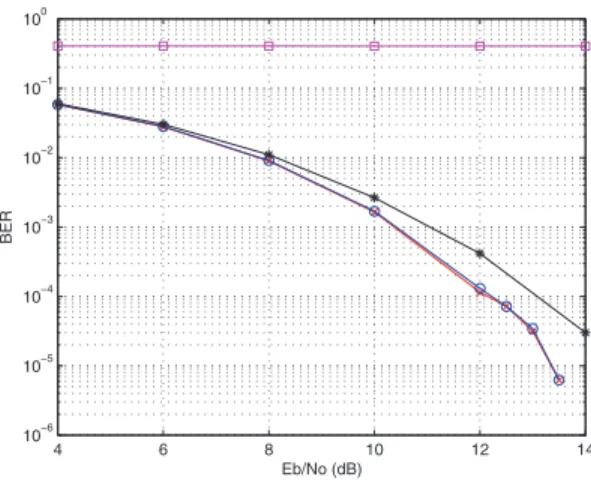
where 𝑃max is the HPA saturation output power and𝑃av is the HPA average output power which is obtained as 𝑃av= E∣𝑑(𝑡)∣2 in the simulation. It is clearly shown in Figure 4 that, while the indirect learning approach can effectively achieve an MSE gain about 30dB, the proposed B-spline approach significantly improves the MSE performance by another 25 ∼ 30dB. This is a significant improvement, indicating that the B-spline approach can almost correct all of the non-linearity effect of the HPA with the Wiener model. Figure 5 shows the bit error rate (BER) performance for the additive white Gaussian noise (AWGN) channel. For comparison, we also show the best possible BER perfor-mance for the ideal case that the HPA introduces no distortion at all (denoted as “Perfect linear HPA” in the figure). It is clearly shown in Figure 5 that the BER performance of the proposed B-spline approach is almost identical to that for the ideal case, and is significantly better than that of the indirect
4 6 8 10 12 14 10−6 10−5 10−4 10−3 10−2 10−1 100 Eb/No (dB) BER
Fig. 5. BER performance for the AWGN channel.
approach. Note that only a single user AWGN channel is considered here as the details of more specific channels are beyond the scope of this paper.
VI. CONCLUSIONS
Based on a new B-spline based Wiener system modeling approach for HPA, a novel nonlinear digital baseband predis-torter design has been introduced using direct learning. The complex valued nonlinear static function in the Wiener HPA model has been identified as the two real valued B-spline neural networks, for the amplitude distortion and the phase shift, respectively. The Gauss-Newton algorithm is applied for the parameter estimation, in which the De Boor recursion has been applied to calculate both the B-spline curve and the first order derivatives. The predistorter, acting as the inverse of Wiener system, is derived by calculating the inverse of the complex valued nonlinear static function based the identified Wiener models. The excellent performance and efficiency of the proposed approaches have been demonstrated using numerical simulations.
REFERENCES
[1] L. Ding, G. T. Zhou, D. R. Morgan, Z. Ma, J.S. Kenney, J. Kim, and C. R. Giardina, “A robust digital baseband predistorter constructed using memory polynomials,” IEEE Trans. Communications, vol. 52, pp. 159–165, 2004.
[2] D. Zhou and V. E. DeBrunner, “Novel adaptive nonlinear predistorters based on the direct learning algorithm,” IEEE Trans. Signal Process-ing, vol. 55, pp. 120–133, 2007.
[3] C. H. Lin, H. H. Chen, Y. Y. Yang, and J. J. Chen, “Dynamically optimum lookup table spacing for power amplifier predistortion lin-earisation,” IEEE Trans. Microwave Theory and Techniques, vol. 54, pp. 2118–2127, 2006.
[4] B. Ai, Z. Y. Yang, C. P. Pan, S. G. Tang, and T. T. Zhang, “Ananysis on lut based predistorting method for HPA with memory,”IEEE Trans. Broadcasting, vol. 53, pp. 127–131, 2007.
[5] R. Raich, H. Qian, and G. T. Zhou, “Orthogonal polynomials for power amplifier modeling and predistorter design,” IEEE Trans. Vehicular Technology, vol. 53, pp. 1468–1479, 2004.
[6] D. R. Morgan, Z. X. Ma, J. Kim, M. G. Zierdt, and J. Pastalan, “A generalized memory polynomial model for digital predistortion of RF power amplifiers,”IEEE Trans. Signal Processing, vol. 54, pp. 3852– 3860, 2006.
[7] L. J. Xu, X. G. Wu, M. Zhang, G. Gang, and P. Zhang, “A stable recursive algorithm for memory polynomial predistorter,” in Proc. MILCOM, Orlando, USA, 2007, vol. 5 pages.
[8] E. Abd-Elrady, L. Gan, and G. Kubin, “Distortion compensation of nonlinear systems based on indirect learning architecture,” in Proc 3rd Int. Symp. Communications, Control and Signal Processing, ST. Julians, Malta, 2008, pp. 184–187.
[9] M. C. Chiu abd C. H. Zeng and M. C. Liu, “Predistorter based on frequency domain estimation for compensation of nonlinear distortion in OFDM systems,” IEEE Trans. on Vehicular Technology, vol. 57, pp. 882–892, 2008.
[10] Y. H. Lim, Y. S. Cho, I. W. Cha, and D. H. Youn, “An adaptive non-linear prefilter for compensation of distortion in nonnon-linear systems,” IEEE Trans. Signal Processing, vol. 46, pp. 1726–1730, 2006. [11] Y. Qian and T. Yao, “Structure for adaptive predistortion suitable for
efficient adaptive algorithm application,” Electronic Letters, vol. 38, pp. 1282–1283, 2002.
[12] S. Choi, E. R. Jeong, and Y. H. Lee, “Adaptive predistortion with direct learning based on piecewise linear approximation of amplifier nonlinearity,” IEEE J. Selected Topics in Signal Processing, vol. 55, pp. 397–404, 2009.
[13] A. Hagenblad, L. Ljung, and A. Wills, “Maximum likelihood iden-tification of Wiener models,” Automatica, vol. 44, pp. 2697–2705, 2008.
[14] A. D. Kalafatis, L. Wang, and W. R. Cluett, “Identification of Wiener-type nonlinear systems in a noisy environment,”International Journal of Control, vol. 66, pp. 923–941, 1997.
[15] I. W. Hunter and M. J. Korenberg, “The identification of nonlinear biological systems: Wiener and Hammerstein cascade models,” Bio-logical Cybernetics, vol. 55, pp. 135–144, 1986.
[16] J. C. Gomez, A. Jutan, and E. Baeyens, “Wiener model identification and predictive control of a ph neutralisation process,” IEE Proc. -Control Theory and Applications, vol. 151, no. 3, pp. 329–338, 2004. [17] C. J. Clark, G. Chrisikos, M.S. Muha, A. A. Moulthrop, and C. P. Silva, “Time-domain envelop measurement technique with application to wideband power amplifier modeling,” IEEE Trans. Microwave Theory and Techniques, vol. 46, pp. 2531–2540, 1998.
[18] W. Greblicki, “Nonparametric identification of Wiener systems,”IEEE Transactions on Information Theory, vol. 38, no. 5, pp. 1487–1493, 1992.
[19] D. Westwick, “Identifying MIMO Wiener systems using subspace model identification model identification methods,”Signal Processing, vol. 52, pp. 235–258, 1996.
[20] A. D. Kalafatis, N. Arifinand L. Wang, and W. R. Cluett, “A new approach to the identification of pH processes on the Wiener model,” Chemical Engineering Science, vol. 50, no. 23, pp. 3693–3701, 1995. [21] Y. Zhu, “Distillution column identification for control using wiener model,” inProc. the American Control Conference, San Diego, CA, USA, 1999, pp. 3462–3466.
[22] de Boor, A Practical Guide to Splines, New York: Spring Verlag, 1978.
[23] C. J. Harris, X. Hong, and Q. Gan, Adaptive Modelling, Estimation and Fusion from Data: A Neurofuzzy Approach, Springer-Verlag, 2002.