A Primal-Dual Augmented Lagrangian Penalty-Interior-Point Algorithm for Nonlinear Programming

(1)

Center for Industrial Mathematics (ZeTeM)

A Primal-Dual Augmented Lagrangian

Penalty-Interior-Point Algorithm for

Nonlinear Programming

Dissertation

submitted to University of Bremen for the degree of Dr. rer. nat.

by

Renke Kuhlmann

August 31, 2018

1st Reviewer: Prof. Dr. Christof Büskens, University of Bremen 2nd Reviewer: Prof. Dr. Philip E. Gill, University of California Date of Defense: December 6, 2018

(2)

(3)

iii

Abstract

This thesis treats a new numerical solution method for large-scale nonlinear optimization prob-lems. Nonlinear programs occur in a wide range of engineering and academic applications like discretized optimal control processes and parameter identification of physical systems. The most efficient and robust solution approaches for this problem class have been shown to be sequential quadratic programming and primal-dual interior-point methods.

The proposed algorithm combines a variant of the latter with a special penalty function to increase its robustness due to an automatic regularization of the nonlinear constraints caused by the penalty term. In detail, a modified barrier function and a primal-dual augmented La-grangian approach with an exactℓ2-penalty is used. Both share the property that for certain Lagrangian multiplier estimates the barrier and penalty parameter do not have to converge to zero or diverge, respectively. This improves the conditioning of the internal linear equation systems near the optimal solution, handles rank-deficiency of the constraint derivatives for all non-feasible iterates and helps with identifying infeasible problem formulations. Although the resulting merit function is non-smooth, a certain step direction is a guaranteed descent. The algorithm includes an adaptive update strategy for the barrier and penalty parameters as well as the Lagrangian multiplier estimates based on a sensitivity analysis. Global convergence is proven to yield a first-order optimal solution, a certificate of infeasibility or a Fritz-John point and is maintained by combining the merit function with a filter or piecewise linear penalty function. Unlike the majority of filter methods, no separate feasibility restoration phase is re-quired. For a fixed barrier parameter the method has a quadratic order of convergence. Furthermore, a sensitivity based iterative refinement strategy is developed to approximate the optimal solution of a parameter dependent nonlinear program under parameter changes. It exploits special sensitivity derivative approximations and converges locally with a linear convergence order to a feasible point that further satisfies the perturbed complementarity condition of the modified barrier method. Thereby, active-set changes from active to inactive can be handled. Due to a certain update of the Lagrangian multiplier estimate, the refinement is suitable in the context of warmstarting the penalty-interior-point approach.

A special focus of the thesis is the development of an algorithm with excellent performance in practice. Details on an implementation of the proposed primal-dual penalty-interior-point algorithm in the nonlinear programming solverWORHP and a numerical study based on the CUTEsttest collection is provided. The efficiency and robustness of the algorithm is further compared to state-of-the-art nonlinear programming solvers, in particular the interior-point solversIPOPTandKNITROas well as the sequential quadratic programming solversSNOPTand WORHP.

Keywords Nonlinear Programming·Large-Scale Optimization·Primal-Dual

Penalty-Interior-Point Algorithm_·Augmented Lagrangian Method_·Modified Barrier Method_·Parametric Sensitivity Analysis_·WORHP

(4)

(5)

v

Zusammenfassung

Diese Arbeit behandelt eine neue numerische Lösungsmethode für hochdimensionale nicht-lineare Optimierungsprobleme. Nichtnicht-lineare Optimierung tritt in einem weiten Spektrum an technischen und akademischen Anwendungen auf, wie beispielsweise in diskretisierten Op-timalsteuerungsprozessen oder in der Parameteridentifikation von physikalischen Systemen. Als die effizientesten und robustesten Lösungsansätze für diese Problemklasse haben sich die Sequentielle-Quadratische-Programmierung und der primär-duale Innere-Punkte-Ansatz ergeben.

Der vorgeschlagene Algorithmus kombiniert eine Variante des Letzteren mit einer speziellen Bestrafungsfunktion, um seine Robustheit mittels der automatischen Regularisierung der nichtlinearen Nebenbedingungen durch den Bestrafungsterm zu erhöhen. Im Detail wird eine modifizierte Barrierefunktion und ein sogenannter primär-dualer erweiterter Lagrange Ansatz mit einer exaktenℓ2-Bestrafungsfunktion genutzt. Beide teilen die Eigenschaft, dass für bestimmte Lagrange-Multiplikator-Abschätzungen der Barriere- und der Bestrafungspram-eter nicht gegen Null konvergieren, bzw. divergieren, müssen. Dies verbessert die Kondition des internen linearen Gleichungssystems nahe der optimalen Lösung, handhabt unzureichen-den Rang der Ableitungen der Nebenbedingungen für alle nicht zulässigen Iterierten und hilft unzulässige Problemformulierungen zu identifizieren. Obwohl die resultierende Bewertungs-funktion nicht differenzierbar ist, führt eine spezielle Suchrichtung zu einem garantiertem Abstieg. Der Algorithmus verfügt über adaptive Aktualisierungsstrategien für den Barriere-und Bestrafungsparameter sowie die Lagrange-Multiplikator-Abschätzungen basierend auf einer Sensitivitätsanalyse. Globale Konvergenz zu einer optimalen Lösung ersten Grades, einer Garantie der Unzulässigkeit oder einem Fritz-John-Punkt wird erzeugt durch die Kombination der Bewertungsfunktion mit einem Filter oder einer stückweise linearen Bestrafungsfunktion. Anders als die Mehrzahl der Filtermethoden wird keine zusätzliche Zulässigkeitskorrektur-phase benötigt. Für einen fixierten Barriereparameter ist die Methode lokal quadratisch kon-vergent.

Des Weiteren wird eine iterative sensitivitätsbasierte Verbesserungsstrategie entwickelt, um die optimale Lösung eines parameterabhängigen nichtlinearen Problems bei Änderungen des Parameters zu approximieren. Diese nutzt dabei spezielle Approximationen der Sensitivitäts-ableitungen aus und konvergiert lokal mit einer linearen Konvergenzordnung zu einem zuläs-sigen Punkt, der zusätzlich die gestörte Komplementaritätsbedingung der modifizierten Bar-rieremethode erfüllt. Dabei können Änderungen der aktiven Menge in Form von aktiv zu in-aktiv gehandhabt werden. Aufgrund besonderer Aktualisierungen der Lagrange-Multiplikator-Abschätzungen ist die iterative Verbesserungsstratgie bestens geeignet für den Warmstart des Bestrafungs-Innere-Punkte-Algorithmus.

Ein besonderer Fokus der Arbeit liegt auf der Entwicklung eines Algorithmus mit beson-derer praktischer Performanz. Details einer Implementierung des vorgeschlagenen primär-dualen Bestrafungs-Innere-Punkte-Algorithmus in dem nichtlinearen Optimierungsproblem-löserWORHPund eine numerische Studie basierend auf derCUTEstTestkollektion werden aus-geführt. Die Effizienz und Robustheit des Algorithmus wird weiterhin verglichen mit hochmo-dernen nichtlinearen Lösungsroutinen, im Besonderen mit dem Innere-Punkte-LöserIPOPT

(6)

und KNITRO sowie mit dem Sequentielle-Quadratische-Programmierungs-Löser SNOPT und WORHP.

Schlüsselwörter Nichtlineare Optimierung·Hochdimensionale Optimierung·Primär-Dualer

Bestrafungs-Innere-Punkte-Algorithmus _· Erweiterte Lagrange-Methode _· Modifizierte Barriere-Methode·Parametrische Sensitivitätsanalyse·WORHP

(7)

vii

Danksagung

Die vorliegende Arbeit entstand im Rahmen eines Promotionsstipendiums der Stiftung der Deutschen Wirtschaft (sdw) sowie meiner Tätigkeit als wissenschaftlicher Mitarbeiter am Zen-trum für Technomathematik der Universität Bremen. Ich blicke auf eine intensive und sehr schöne Zeit in der AG Optimierung und optimale Steuerung zurück, während der ich stets von anregenden Diskussionen, einer vertrauensvollen Atmosphäre und kritischen Rückfragen profitieren konnte. Letztlich hat das einen nicht unerheblichen Einfluss auf den Erfolg meiner Dissertation, wofür ich sehr dankbar bin.

Zunächst möchte ich mich bei meinem Doktorvater Christof Büskens bedanken, der mich bereits während des Bachelorstudiums für den Bereich der numerischen nichtlinearen Opti-mierung begeisterte und mir schon früh die Chance gab in die Entwicklung der SoftwareWORHP einzusteigen. Er garantierte stets einen idealen Rahmen für die Promotion, der unter anderem viel Freiraum bei der Umsetzung eigener Ideen bot. Weiterhin danke ich Christoph Buchheim und Christian Meyer, die mich persönlich und wissenschaftlich sehr unterstützt haben. Von ihnen konnte ich viele nutzbringende Kenntnisse über das wissenschaftliche Arbeiten und Publizieren erlernen und Erfahrungen sammeln. Mein Dank gilt ferner Philip E. Gill für das Interesse an meiner Arbeit und die Übernahme des Zweitgutachtens.

Ich danke allen Kolleginnen und Kollegen der AG Optimierung und optimale Steuerung für die hervorragende Arbeitsatmosphäre, insbesondere aber natürlich den weiterenWORHP Ent-wicklern Matthias Knauer, Jan Niklas Hasse, Marcel Jacobse und Sören Geffken für die tolle Zusammenarbeit. Den beiden letztgenannten bin ich darüber hinaus im Besonderen zu Dank verpflichtet, da sie die vorliegende Arbeit Korrektur lasen.

Am allermeisten aber möchte ich mich bei meiner Familie bedanken. Die Unterstützung und Förderung meiner Eltern Margot und Erhard Schäfer ist unermesslich und legte den Grund-stein für ein erfolgreiches Studium. Ich danke meiner Schwester Rieke Trimçev, die für mich ein akademisches Vorbild ist und mich letztlich auf die Idee brachte Technomathematik zu studieren. Außerdem danke ich meiner Partnerin Nele Kuhlmann für die Ermutigungen, den Rückhalt und das Verständnis besonders in den intensiven und frustrierenden Phasen der Dis-sertation sowie für ihre Initiative Fiete bei uns aufzunehmen. Dieser Hund ist einfach der ideale Gefährte für einen Wissenschaftler wie mich.

(8)

(9)

List of Acronyms

BLAS Basic Linear Algebra Subroutines . . . 173

CQ Constraint Qualification . . . 14

FJ Fritz-John[conditions] . . . 16

KKT Karush-Kuhn-Tucker[conditions] . . . 15

LICQ Linear Independence Constraint Qualification . . . 14

MFCQ Mangasarian-Fromovitz Constraint Qualification . . . 14

MPEC Mathematical Program with Equilibrium Constraints . . . 31

NLP Nonlinear Problem, Nonlinear Program or Nonlinear Programming . . . . 9

PDE Partial Differential Equation . . . 4

PLPF Piecewise Linear Penalty Function . . . 44

QP Quadratic Program or Quadratic Programming . . . 32

SCC Strict Complementarity Condition . . . 18

SLP Sequential Linear Programming . . . 34

SOSC Second-Order Sufficient Condition . . . 18

SQP Sequential Quadratic Programming . . . 32

(14)

(15)

List of Figures

2.1 Local and global optimal solution and global certificate of infeasibility of

Exam-ple 2.3. . . 11

2.2 Geometric interpretation of optimality conditions for Example 2.4. . . 13

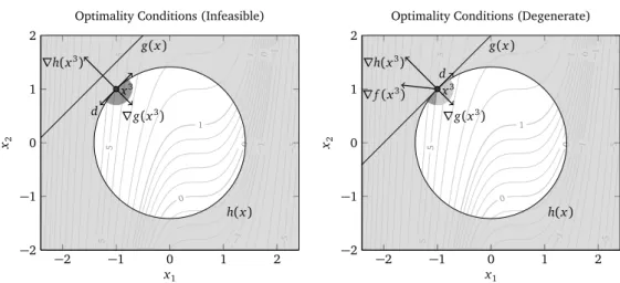
2.3 Geometric interpretation of optimality conditions for the infeasible and degen-erate case of Example 2.19. . . 17

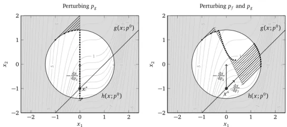
2.4 Sensitivities and first-order approximations for perturbations of Example 2.32. . 26

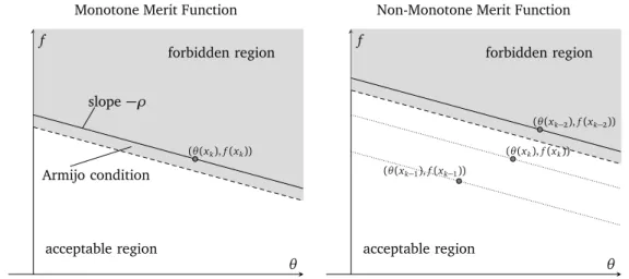
3.1 Monotone and non-monotone merit function. . . 39

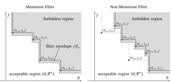
3.2 Monotone and non-monotone filter. . . 41

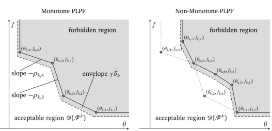
3.3 Monotone and non-monotone PLPF. . . 45

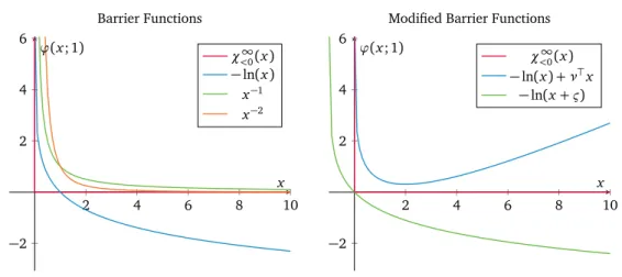
3.4 Different barrier functions and modified barrier functions. . . 51

3.5 Central path for Example 2.3 based on log-barrier function. . . 52

3.6 Penalty function path for Example 2.3 based onℓ2-penalty function. . . 57

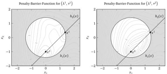
4.1 Optimal solution of Example 4.1 with corresponding penalty-interior-point ob-jective function. . . 70

4.2 Non-monotone filter and non-monotone PLPF combined with non-monotone merit function. . . 81

4.3 Perturbed central path for Example 2.3 based on log-barrier function. . . 135

4.4 Optimal solution and sensitivity derivatives of the nonlinear program of Exam-ple 4.42. . . 148

4.5 Approximation of the nonlinear program of Example 4.42 generated by warm-start based on iterative real-time updates. . . 148

5.1 Performance profile for numerical study of the initialization strategies. . . 158

5.2 Individual performance profiles for numerical study of the initialization strategies.158 5.3 Performance profile for the numerical study of the linear equation system solu-tion strategies. . . 162

(16)

5.4 Individual performance profiles for the numerical study of the linear equation system solution strategies. . . 162 5.5 Performance profile for the numerical study of the line search strategies. . . 166 5.6 Individual performance profiles for numerical study of the line search strategies. 167 5.7 Performance profile for the numerical study of the modified and classic barrier

function and adaptive parameter updates. . . 171 5.8 Individual performance profiles for the numerical study of the modified and

classic barrier function and adaptive parameter updates. . . 171 5.9 Performance profile for the numerical study of the modified and classic barrier

function when warmstarting. . . 172 5.10 Individual performance profiles comparing the altered performance of NLP

solversIPOPT,KNITROandWORHP SQPdue to configuration changes. . . 174 5.11 Performance profile for the numerical study of the nonlinear programming

solversIPOPT,KNITRO,SNOPT,WORHP IP,WORHP IPmandWORHP SQP. . . 175 5.12 Individual performance profiles for the numerical study of the nonlinear

pro-gramming solversIPOPT,KNITRO,SNOPT,WORHP IP,WORHP IPmandWORHP SQP. 176 5.13 Performance profile for the numerical study of the nonlinear programming

solversIPOPT,KNITRO,SNOPT,WORHP IP,WORHP IPmandWORHP SQP. . . 178 5.14 Individual performance profiles for the numerical study of the nonlinear

pro-gramming solversIPOPT,KNITRO,SNOPT,WORHP IP,WORHP IPmandWORHP SQP. 179 5.15 Performance profile for the numerical study of the crossover. . . 181 5.16 Individual performance profiles for the numerical study of the crossover. . . 181

(17)

List of Tables

4.1 Iterations of feasibility and complementarity refinement for Example 4.42 with active set change from active to inactive. . . 146 4.2 Iterations of feasibility and complementarity refinement for Example 4.42 with

active set change from inactive to active. . . 147 5.1 Numbers of termination statuses for the numerical study of the initialization

strategies. . . 157 5.2 Numbers of termination statuses for the numerical study of the linear equation

system solution strategies. . . 161 5.3 Numbers of termination statuses for the numerical study of the line search

strategies. . . 165 5.4 Numbers of termination statuses for the numerical study of the modified and

classic barrier function and adaptive parameter updates. . . 170 5.5 Numbers of termination statuses for the numerical study of the modified and

classic barrier function when warmstarting. . . 172 5.7 Numbers of termination statuses for the numerical study of the nonlinear

pro-gramming solversIPOPT,KNITRO,SNOPT,WORHP IP,WORHP IPmandWORHP SQP. 173 5.6 Altered parameter configuration of NLP solvers IPOPT, KNITRO, SNOPT and

WORHP SQP. . . 174 5.8 Numbers of termination statuses for the numerical study of the nonlinear

pro-gramming solversIPOPT,KNITRO,SNOPT,WORHP IP,WORHP IPmandWORHP SQP on infeasibleCUTEstversion. . . 177 5.9 Numbers of termination statuses for the numerical study of the crossover. . . 180 B.1 Overview of solver status outcomes of the nonlinear programming solvers

IPOPT,KNITRO,WORHP IP,WORHP IPmandWORHP SQPon theCUTEsttest set. . . 192 B.2 Comparison of the nonlinear programming solversIPOPT,KNITRO, WORHP IP,

WORHP IPmandWORHP SQPon theCUTEsttest set. . . 293

(18)

(19)

List of Algorithms

A Locally Convergent Lagrange-Newton Method for Equality Constrained Programs 29

B Locally Convergent SQP Method . . . 33

C Locally Convergent Sensitivity Based Recursive Algorithm . . . 34

D Globally Convergent SQP Method (Merit Function) . . . 40

E Globally Convergent SQP Method (Filter) . . . 43

F Locally Convergent Active-Set Method . . . 49

G Locally Convergent Primal-Dual Interior-Point Method . . . 54

H Locally Convergent Primal-Dual Penalty Method for Equality Constrained Pro-grams . . . 58

I Real-Time Approximation with Feasibility Corrections . . . 62

J Second-Order-Correction Steps . . . 64

K Locally Convergent Modified Lagrange-Newton Method . . . 65

L Primal-Dual Augmented Lagrangian Penalty-Interior-Point Algorithm . . . 90

M One Iteration of Adaptive Updates for the Primal-Dual Penalty-Interior-Point Algorithm . . . 134

N Iterative Real-Time Update Based Warmstart . . . 138

O Primal Regularization . . . 161

(20)

(21)

Chapter 1

Introduction

«Roughly speaking, local optimization methods are more art than technology. Local optimization is well developed art, and often very effective, but it is nevertheless an art.»

Boyd and Vandenberghe_[23, p. 9_] Optimization can be found almost everywhere. It is a fundamental principle in nature and a valuable tool for humans to improve their actions and making. No matter if an engineering application considers an automotive, a robot or a space rocket for example, they often share the endeavor to minimize energy consumption and environmental influences – which is often directly linked to the minimization of costs. If these costs can be specified or modeled as a func-tion of decision variables, a mathematical optimizafunc-tion problem is defined. It usually contains some kind of restrictions for the decision variables, which are mathematically expressed as constraint functions. While it is the task of practitioners to model their real-world application as a set of these usually nonlinear cost and constraint functions, it is the goal of mathematical optimization to find the optimal decision variables that minimize the cost or objective function. A subsequent scientific research question is how this optimal solution changes under pertur-bations of model parameters. These parameters appear in almost every optimization problem with a value that could be uncertain or for which different configurations need to be consid-ered. A sensitivity analysis[60, 61]provides these insights and thus enables to approximate

the optimal solution of the perturbed optimization problem.

Solving optimization problems with arbitrary nonlinear functions can be difficult both in the-ory and in practice. Complexity occurs due to non-convexity of functions, which implies ex-istence of multiple solutions with different quality or – in other words – many local minima, and due to inequality constraints (cf.,[172]). In particular the former may have motivated

some researches (cf.,[23]) to see nonlinear optimizers as artists because of the challenging

task to compose practical algorithms to find good quality local solutions. Inequality constraints could be handled efficiently as equality constraints if the active set, i.e., the set of inequality constraints that are satisfied with equality, would be known for the optimal solution. Since

(22)

this is usually not the case, numerical solution strategies like active-set[47, 58, 108],

interior-point[37, 64, 77, 79], penalty[64, 116, 164]and sequential quadratic programming methods [19, 90, 192]have been developed, where the given references are just a very limited

selec-tion. While active-set approaches iteratively estimate the optimal active set when progressing towards the optimal solution and setting variables that are considered to be active to their bound value, interior-point methods add a sequentially decreasing barrier to the objective function to prevent constraints from becoming active during the process. Penalty methods are similar in the sense that they add a penalty to the objective function, but only if constraints are violated. Sequential quadratic programming is a different concept as it sequentially approxi-mates the optimization problem using a quadratic model that is solved by either of the other methods – mainly active-set.

When comparing state-of-the-art nonlinear programming solvers, interior-point methods turn out to be the most efficient[13, 142, 143].1However, despite the development of many

differ-ent practical interior-point algorithms[29, 185, 202]within the last two decades, some aspects

still leave room for improvements: How to handle degeneracy of constraint functions, i.e., lin-ear dependent gradients? How to quickly detect if a problem formulation is infeasible? And, how to warmstart an interior-point algorithm to solve a sequence of similar optimization prob-lems efficiently? These research questions are of particular interest if interior-point algorithms shall serve as local solvers within global (mixed-integer) nonlinear programming methods, a field that is usually dominated by sequential quadratic programming methods[89, 144].

1.1 Thesis Aims and Contribution

The thesis firstly aims to survey the theory and existing numerical methods of derivative based optimization techniques to solve smooth nonlinear optimization problems. The main goal, however, is the design and development of a new primal-dual augmented Lagrangian penalty-interior-point algorithm that addresses the above research questions and is efficient in practice. A practical implementation of that algorithm within the nonlinear programming solverWORHP

[36]is provided. The method is thoroughly studied theoretically and numerically.

The primal-dual augmented Lagrangian penalty-interior-point algorithm combines a modified barrier function[46, 97, 162]with an augmented Lagrangian penalty[116, 164]to solve the

constrained nonlinear optimization problem as an unconstrained one. While the interior-point approach guarantees the high efficiency of the method, the additional penalty increases its robustness. This is due to an automatic dual regularization that handles degenerate constraint gradients similar to_[2, 40, 43, 95, 97_]. Unlike the majority of augmented Lagrangian based methods, an exact and non-smooth ℓ2-penalty is used [40, 42, 43] that includes a natural

adaptive penalty parameter update strategy. A further penalty parameter multiplying the ob-jective function follows[31, 67]and improves the quick detection of infeasibility. The special

barrier-penalty combination benefits from barrier and penalty parameters that do not require

1_{The referenced benchmarks consider the one-time optimization of feasible nonlinear programs exploiting first}

and second-order derivatives when possible for a solver. The statement may change in favor of sequential quadratic programming methods if these assumptions are modified, cf.,_[92_].

(23)

1.1. Thesis Aims and Contribution 3

converging to zero. Whereas recent research trends[101, 136]try to avoid a merit function or

filter approach as line search globalization, the proposed method combines the two. The merit function is essential for theoretical convergence and the filter, originally developed by[69],

massively increases the step acceptance rates and thus improves the practical performance. However, most filter algorithms (e.g., [183, 202]) require a separate feasibility restoration

phase. Due to the combination with the merit function, this is not required for the proposed method, which results in faster detection of infeasibility. A further advantage of the proposed filter is the independence on any of the involved barrier or penalty parameters.

A global convergence analysis proves that the algorithm converges for an arbitrary initial guess to either an optimal solution, a certificate of infeasibility or a Fritz-John point under standard assumptions. A vital element is the proof of a guaranteed descent direction for the non-smooth barrier-penalty merit function for a modified Newton step. Proofs for fast local convergence of the underlying penalty approach and asymptotic convergence orders when approaching an optimal solution or certificate of infeasibility conclude the theoretical analysis. Most of these proofs follow the presentations of similarℓ2[6, 40, 42, 43]or augmented Lagrangian[2, 3,

155_] based penalty-interior-point algorithms, but are translated or extended to the barrier-penalty combination considered in this thesis.

Furthermore, the thesis provides an extensive study of applying sensitivity analysis as an in-ternal tool to improve efficiency besides showing how to calculate sensitivity derivatives for classic post-optimality sensitivity analysis at low computational cost. Among them are comple-mentarity refinement steps and adaptive barrier and penalty parameter updates. For the latter, sensitivity derivatives can indicate in every iteration of the algorithm which parameter update provides best progress towards an optimal solution and by that offers a highly flexible update scheme. This is similar to[48, 153], but has not been studied for a modified barrier function

before, which requires further considerations.

A new warmstart approach for modified barrier based interior-point algorithms is proposed. It uses sensitivity derivatives in an iterative feasibility and complementarity refinement to ap-proximate the optimal solution of the new perturbed optimization problem. It is proven that the method convergences to a point that satisfies the perturbed feasibility and complementar-ity condition of the barrier-penalty subproblem with a linear convergence order. This approach is a great advancement over classic real-time updates as it features certain active set changes. It can therefore be seen as the interior-point perspective on a task that is usually addressed by active-set approaches[123, 161, 193, 205]. Sensitivity information can be transferred to

the Lagrangian multiplier estimates in the modified barrier function with a suitable projec-tion to provide a good starting point for warmstarting a modified barrier based interior-point algorithm.

The aim of the numerical study is to provide insights that determine the algorithm components with the highest impact on the practical performance and to prove the high efficiency and ro-bustness of the developed method by comparing it to the state-of-the-art interior-point and sequential quadratic programming solversIPOPT_[202_],KNITRO_[29_],SNOPT_[91_]andWORHP

[36] on theCUTEsttest set_[107_]. A special emphasis is also put on a performance compari-son on infeasible problem formulations showing the superiority of the proposed method over the other interior-point solvers. Finally, a crossover is designed that offers the possibility to

(24)

switch from the penalty-interior-point algorithm toWORHP’s sequential quadratic programming method at an arbitrary iteration of the optimization process.

Contributions to Publications

During the creation of this thesis, the author contributed to five publications, of which three are directly connected to the content of this work. A brief overview is given in the following.

[25] C. Buchheim, R. Kuhlmann, and C. Meyer. Combinatorial optimal control of

semilin-ear elliptic PDEs. Computational Optimization and Applications, 70(3):641–675, 2018. doi:10.1007/s10589-018-9993-2

The paper considers a novel outer approximation approach for the efficient solution of optimal control problems with semilinear elliptic partial differential equations (PDEs) and static inte-ger controls over arbitrary combinatorial structures. This problem class is difficult in practice and is usually addressed by a domain discretization, which leads to very large-scale mixed-integer nonlinear programs. The proposed algorithm, however, is based on a decomposition of the optimal control problem into an efficiently solvable integer linear programming master problem and a cutting plane generating subproblem. The latter relies on a pointwise concavity or submodularity of the PDE solution with respect to the integer controls. Such a sequential framework allows exploiting reoptimization techniques for solving the PDE. The paper includes a numerical study that shows the efficiency of the proposed approach.

Kuhlmann’s main contribution is the development of reoptimization strategies for an efficient PDE solution, aMatlabimplementation of the proposed algorithm and the numerical study in the paper. Although the publication is not directly linked to this thesis, it motivated many algo-rithmic considerations. Following the generic domain discretization approach for the solution of a PDE with inequality state constraints, an interior-point method would probably be the best choice for the resulting large-scale nonlinear program. The inclusion into a mixed-integer solution framework would then require certain features like fast detection of infeasibility and ability to warmstart that are usually considered to be a weakness of interior-point methods.

[129] R. Kuhlmann and C. Büskens. A primal–dual augmented Lagrangian

penalty-interior-point filter line search algorithm. Mathematical Methods of Operations Research, 87(3): 451–483, 2018. doi:10.1007/s00186-017-0625-x

In this journal article a primal-dual penalty-interior-point algorithm based on the combination of a classic log-barrier and an augmented Lagrangian approach with an exactℓ2-penalty is considered to solve generic nonlinear programs. Special emphasis is placed on the practical performance of the detection of infeasibility and of the line search strategy that combines a filter with a merit function. Unlike the majority of filter methods, this does not require a separate feasibility restoration phase. This publication is closely linked to this work, as one part of this thesis is the extension of the algorithm – among many smaller improvements – by a modified barrier function.

(25)

1.1. Thesis Aims and Contribution 5

[130] R. Kuhlmann, S. Geffken, and C. Büskens. WORHP Zen: Parametric sensitivity

anal-ysis for the nonlinear programming solver WORHP. In N. Kliewer, J. F. Ehmke, and R. Borndörfer, editors, Operations Research Proceedings 2017, pages 649–654. Springer International Publishing, 2018. doi:10.1007/978-3-319-89920-6_86

The conference paper presents the practical parametric sensitivity analysis moduleWORHP Zen of the nonlinear programming solverWORHP. Sensitivity derivatives with respect to parameter data are of high interest because they improve the understanding of the optimal solution and allow the formulation of real-time capable update algorithms. Besides showing implementa-tion details for the efficient calculaimplementa-tion as well as sparse storage of parametric sensitivities and the real-time updates, the paper illustrates the application ofWORHP Zen in the field of parameter identification.

As the development ofWORHP Zenbegan with Schäfer _[174_] the author’s main contribution was the efficientFortranimplementation inWORHPand the presentation of implementation details.

[144] B. Müller, R. Kuhlmann, and S. Vigerske. On the performance of NLP solvers within

global MINLP solvers. In N. Kliewer, J. F. Ehmke, and R. Borndörfer, editors, Oper-ations Research Proceedings 2017, pages 633–639. Springer International Publishing, 2018. doi:10.1007/978-3-319-89920-6_84

In this conference paper the performance of nonlinear programming solvers are studied when applied to the internal subproblems of the mixed-integer nonlinear programming solverSCIP. Among them are primal heuristics, convex relaxations and bound tightening methods. Kuhlmann contributed in the development of theWORHPinterface inSCIP, which included an adaptation of the warmstarting interface ofWORHP, and extended the interior-point algorithm ofWORHPwith different warmstarting strategies.

[173] M. Schweinoch, R. Schäfer, A. Sacharow, D. Biermann, and C. Buchheim. A non-rigid

reg-istration method for the efficient analysis of shape deviations in production engineering applications. Production Engineering, 10(2):137–146, 2016. doi:10.1007/

s11740-016-0660-0

The paper studies a new non-rigid registration method for the efficient calculation of corre-spondences of designed and as-built parts in production engineering applications. Non-rigid registration methods are based on a deformation of the one geometry onto the other. The proposed method combines an error-adaptive segmentation with rigid alignments of each seg-ment and a restoration of connectivity by minimizing a mesh energy functional. The paper includes a numerical study where the method is applied to the problem of springback in sheet metal forming.

Kuhlmann’s main contribution was the development and implementation of the energy func-tional optimization for restoring mesh connectivity.

(26)

1.2 Thesis Overview

The thesis is partitioned into four main chapters.

The Chapter 2 gives an overview of the theoretical foundations in nonlinear programming. After the definition of the problem task and its optimal solution, necessary and sufficient con-ditions for the characterization of an optimal solution are derived in Section 2.1 with a special emphasis on the first-order necessary conditions as these are extensively used by numerical algorithms. On this basis, the chapter continues with the theory of parametric sensitivity analy-sis in Section 2.2. This includes the derivation of first- and second-order sensitivity derivatives and the approximation of perturbed nonlinear programs.

Chapter 3 treats the question of how to solve nonlinear optimization problems numerically by studying the proposed approaches in the literature. The focus is on derivative based methods that apply Newton’s method to the first-order necessary conditions as motivated in Section 3.1. This requires developing schemes for the globalization (Section 3.3) and regularization (Sec-tion 3.4) of this special variant of Newton’s method. Nevertheless, inequality constraints cannot be handled by this approach directly and strategies to simplify these and to solve optimization problems with inequality constraints are presented in Section 3.2 and Section 3.5, respectively. Among them are active-set, interior-point or barrier and exterior-point or penalty methods. The final Section 3.6 of this chapter considers sensitivity analysis based techniques to increase the efficiency or robustness of numerical optimization algorithms.

The Chapter 4 presents the proposed primal-dual augmented Lagrangian penalty-interior-point algorithm. After a brief theoretical study of the combined penalty-barrier function in Section 4.1, the main ingredients of the algorithm, i.e., step computation, line search, pa-rameter updates and a so called magic step, are introduced and discussed in Section 4.2. A convergence analysis studies the theoretical properties of the algorithm far away from the optimal solution (global convergence, Section 4.3) and very close to it (local convergence, Section 4.4). In the remainder of the chapter, the sensitivity analysis is widely applied to the proposed penalty-interior-point algorithm. In Section 4.5 sensitivity derivatives of optimiza-tion variables with respect to the original, the barrier sub- and the barrier-penalty subproblem are derived. Sensitivity derivatives of the step direction are the basis for adaptive barrier and penalty parameter updates in Section 4.6. Finally, Section 4.7 proposes an iterative refinement strategy using sensitivity information for an improved warmstart of a modified barrier function based interior-point algorithm.

In Chapter 5 a description of a practical implementation of the proposed penalty-interior-point algorithm within the nonlinear programming solver WORHP and numerical results are provided. After a brief introduction of the solverWORHPand theCUTEsttest collection as well as benchmark metrics (Section 5.1), detailed algorithmic considerations and enhancements for a good practical performance are studied in Section 5.2. A comparison to state-of-the-art nonlinear programming solvers completes the chapter in Section 5.3.

(27)

1.3. Notation 7

1.3 Notation

Scalars and vectors are written in lowercase and matrices in uppercase. The letters are either Roman or Greek and squared brackets are used for its definition, e.g.,A:=1 2 3∈N1×3.

For a given vectorb_∈Rnwithn∈Nthe uppercase version Bis defined as a square diagonal

matrix withbon its diagonal, i.e.,B:=diag(b)∈Rn×n. Theith element of the vector bisbi and, thus, theith unit vector of appropriate size iseiwhereej=1 ifi= jandej=0 otherwise. Following this approach,eis defined as a vector of ones andE:=diag(e)is the identity matrix.

As for the unit vector and the identity matrix the size is not specified for the zero vector or zero matrix 0, but will be evident from the context. A comparison of two vectors – e.g., lesser, greater or equal – is always defined to be element-wise, i.e.,a_≤ bwith two vectorsa,b_∈Rn

is equivalent toa_i _≤ b_i for all i₌ 1, . . . ,n. A tuple of vectors c_{= (}a,b₎_∈Rn×Rm will also

be accessed as the vectorc ₌a⊤ _b⊤⊤ _∈

Rn+m. The norm of a vector or matrix is∥·∥ and

may be any of the possible vector or matrix norms unless specified, e.g.,_∥·∥2for the Euclidean norm and_∥·∥_∞for the maximum norm. Analogously,_|·|is the absolute value of a scalar. Sets are written in calligraphic font and are defined using curly brackets, e.g.,A :={1, 2, 3}.

The only exception to this rule are the number sets. The most important ones areN andN0 for natural numbers without or with zero as well asR,R0+andR+ for real, non-negative real

and strictly positive real numbers. The empty set is_; and the number of elements of _A is |A |. A ball around a point b_∈Rn with radiusϵ >0 is defined asBϵ(b). If the radius is of

no further relevance and just assumed to be sufficiently small or the shape is not necessarily a ball, a neighborhood written as_N(b)is used. To simplify notation, the neighborhood around

a tuple(a,b)is equivalently referred to asN((a,b)) =N(a,b)and analogously for a ball.

Sequences of scalars are written as{a_k_}_k_∈_N₀_⊆R, of vectors as

ak

k∈N0⊆R

n _{and of matrices} as_{A_k_}_k_∈_N₀_⊆Rn×m to avoid confusion with theith element of a vector. If the index set isN0 the definition is abbreviated to{a_k_}_k and similar for vectors and matrices. For a given index set_K the notation is also simplified to_{a_k_}_K. Furthermore, the Landau notation is utilized.

Definition 1.1 (Landau Notation). Let_{a_k_}_k_⊆R0+ and {bk}k⊆ R0+ be two sequences with non-negative elements. The Landau notation is defined as:

– a_k₌_O₍b_k₎if a_k is bounded above by b_k asymptotically, i.e.,lim sup_k_→∞|ak|

|bk| <∞or –

in other words – if there exists c>0such that ak≤c bkfor k∈Nlarge enough. – ak=Ω(bk)if akis bounded below by bkasymptotically, i.e., bk=O(ak).

– a_k₌Θ(bk)if ak is bounded both above and below by bk asymptotically, i.e., ak=O(bk) and ak=Ω(bk).

– ak=o(bk)if ak is dominated by bk asymptotically, i.e.,limk→∞||abkk|| =0or if there exists

a sequence_{c_k_}_k_∈_N_⊆Rthat converges to zero such that ak=ckbkfor k∈Nlarge enough.

Special cases of the Landau notation are ak = Θ(1)and ak = o(1)to state that a sequence {a_k_}_k_⊆R0+is bounded away from zero – at least for large indicesk– and bounded above or

(28)

Derivatives of sufficiently smooth functions f :Rn×Rm→Randg:Rn→Rm– also referred

to as g_i :Rn →Rwithi=1, . . . ,m– for x ∈Rn and y ∈Rm evaluated at the points ¯x ∈Rn

and ¯y _∈Rmare defined as

∇xf(¯x, ¯y):= _∂_f ∂x1(¯x, ¯y) . . . ∂f ∂xn(¯x, ¯y) _⊤ ∈Rn ∇xg(x¯):= ⎡ ⎢ ⎣ ∂g1 ∂x1(x¯) . . . ∂gm ∂x1 (x¯) ... ... ... ∂g1 ∂xn(x¯) . . . ∂gm ∂xn (x¯) ⎤ ⎥ ⎦∈Rn×m and consequently ∇2x yf(¯x, ¯y):=∇y ∂f ∂x1(x¯, ¯y) . . . ∂f ∂xn(¯x, ¯y) _⊤ = ⎡ ⎢ ⎢ ⎣ ∂2f ∂x1∂y1(¯x, ¯y) . . . ∂2f ∂xn∂y1(¯x, ¯y) ... ... ... ∂2f ∂x1∂ym(¯x, ¯y) . . . ∂2f ∂xn∂ym(¯x, ¯y) ⎤ ⎥ ⎥ ⎦, where ∂

∂xi are partial derivatives with respect to xi,i=1, . . . ,n. The short notation∇g(x¯)is

used for the Jacobian matrix∇xg(¯x), because it is the only derivable variable in this case. For a function gi(x)withi =1, . . . ,mthe derivative∇gi(¯x) is called the gradient and∇2gi(¯x) the Hessian matrix. For a non-smooth but convex function h : Rn → R the subdifferential

evaluated at ¯x_∈Rn is∂xh(¯x).2

Finally,(·)+is a short notation for max{0,·}. A list of all symbols defined throughout the thesis

is provided at the end of the work.

(29)

Chapter 2

Nonlinear Programming

The focus of attention in mathematical optimization is the minimization of anobjective function f₍x₎subject toequality constraints g₍x_{) =}0 andinequality constraints h₍x₎_≤0, wherex are the so calledoptimization variables. In nonlinear programming the three functions f₍x₎, g₍x₎

orh(x)may be nonlinear and possibly non-convex1. This work uses the formal definition of a

nonlinear optimization problem ornonlinear program(NLP) min x∈Rnx f(x) subject to g(x) =0 h(x)≤0 (NLP)

with twice continuously differentiable functions f : Rnx → R, g : Rnx → Rng and h:Rnx →Rnh.2 The term large-scale optimization refers to nonlinear programs (NLP) with

a large number of optimization variablesn_x or number of constraintsn_g orn_h. It is possible to maximize a function f(x)by considering the minimization of−f(x).

For further expositions, the following basic definitions are necessary. A point x that satisfies the constraints g(x) = 0 and h(x) ≤ 0 is called feasible and the feasible set is defined as D:= {x ∈Rnx |g(x) =0 andh(x)≤0}. Accordingly, a point x is said to beinfeasibleif it is

not feasible, i.e.,x _{̸∈ D}. Furthermore, an inequality constraint is defined to beactive, if it takes the value of its bound andinactiveif it is bounded away from it. Consequently, theactive set

is defined asA(x):={i|hi(x) =0}and theinactive setasI(x):={1, . . . ,nh} \ A(x). The goal of the optimization is to find theoptimal solutionof (NLP) defined as follows.

Definition 2.1 (Optimal Solution). A feasible point x∗∈ D is called i. global optimal solution, if f₍x∗₎_≤ _f₍_x₎_{for all x}_{∈ D}_.

ii. local optimal solution, if there existsϵ >0such that f(x∗)≤ f(x)for all x∈ D ∩Bϵ(x∗).

1_{For a formal definition of non-convexity of a function, see Definition A.11.}

2_{The twice continuously differentiable condition of the functions}_f₍_x₎_,_g₍_x₎_and_h₍_x₎_{will be assumed}

through-out the presentation. Although it will not be stated at all times, it will be clear from the usage of derivatives that this condition must hold.

(30)

If the condition is satisfied with f₍x∗₎_< _f₍_x₎_{for x}_̸₌_x∗_{, the point is called strict global or strict} local optimal solution, respectively.

Finding the global optimal solution of the nonlinear program (NLP) is in general extremely difficult. In fact, it is NP-hard. This means that if P̸=NP3, the problem cannot be solved

effi-ciently in polynomial time on a deterministic Turing machine. Sahni[172, Theorem 2.5.4], for

example, proved this result for the special case of non-convex quadratic programming, which is a subset of nonlinear programming. Therefore, and because global solution algorithms of-ten require an efficient local solver, this thesis aims to find local optimal solutions of (NLP). For surveys on global optimization, the reader is referred to Floudas[74], Hansen and

Wal-ster[115]and Pardalos and Rosen[158]. In the special case of convex functions f(x), g(x)

andh(x), local optimal solutions are always global optimal solutions (cf., Geiger and Kanzow

[84, Theorem 2.46]). For convenience, the shorter term optimal solutionis used to refer to

a local optimal solution x∗ _{and the definitions} _f∗ _:₌ _f₍_x∗₎_, _g∗ _:₌ _g₍_x∗₎_, _h∗_:₌ _h₍_x∗₎ _{– and}

analogously for variables and functions defined later on – are utilized.

It may not always be possible to find an optimal solution x∗ _{of (NLP) since the equality}

con-straints g(x) =0 could be violated for allx satisfying the inequality constraintsh(x)≤0 and thus _D = ;.4 _{In these cases it is desirable to find at least the point for which the}_constraint

violation _∥g₍x₎_∥ is minimized, i.e., finding the optimal solution of the following feasibility problem:

min x∈Rnx ∥

g₍x₎_∥2

subject to h(x)≤0 (FeasNLP)

It has to be noted, that this definition does not satisfy the definition of the nonlinear op-timization problem (NLP) since its objective function is not differentiable on the whole domain. However, the definition of the feasibility problem is only applied for infeasible points x with _∥g₍x₎_∥>0 where the twice continuously differentiability condition holds. It is of course possible to formulate different feasibility problems, e.g., the smooth adaptation min_x_∈_Rnx_,_h₍_x₎_≤₀∥g(x)∥2₂, but (FeasNLP) will harmonize well with the algorithm proposed in

Chapter 4. Furthermore, for a definition of (FeasNLP) to make sense, the existence of a neigh-borhood has to be assumed for which the inequality constraintsh(x) ≤ 0 can be satisfied –

actually an assumption of the just mentioned algorithm. In analogy to the optimal solution of (NLP), acertificate of infeasibilityis defined.

Definition 2.2 (Certificate of Infeasibility). A point x∗ with∥g(x∗)∥>0and h(x∗) ≤0is called

i. global certificate of infeasibility, if_∥g(x∗)∥ ≤ ∥g(x)∥for all x_∈Rnx with h(x)≤0.

3_{P and NP are complexity classes and if P equals NP is an open question of complexity theory, but for this}

presentation just the following is relevant. If it was true, the difficult problems contained in NP would be solvable efficiently in polynomial time (similar to problems in P).

4_{It is of course also possible that there is no point}_x_{that satisfies the inequality constraints, i.e.,}_h₍_x₎_>_{0 for all}

x. That case will however not be considered in the presentation since it does not occur for the proposed algorithm due to a reformulation (cf., Section 3.2.1).

(31)

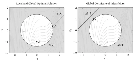
2.1. Optimality Conditions 11 5 5 5 5 1 1 1 0 0 0 0 −1 −1 −1 −1 −5 − 5 −5 −5 g(x) h(x) x1 x2 −2 −1 0 1 2 −2 −1 0 1 2 x1 x2

Local and Global Optimal Solution

5 5 5 5 1 1 1 0 0 0 0 −1 −1 −1 −1 − 5 − 5 − 5 −5 g(x) h(x) x3 −2 −1 0 1 2 −2 −1 0 1 2 x1 x2

Global Certificate of Infeasibility

Figure 2.1:Local and global optimal solution and global certificate of infeasibility of Example 2.3. The objective

function is plotted as level set. Left: Optimal solution forpg=1; Right: Certificate of infeasibility forpg=2.5. The

infeasible region with respect to the inequality constraint is the light gray area.

ii. local certificate of infeasibility, if there existsϵ > 0such that _∥g(x∗)∥ ≤ ∥g(x)∥ for all x_∈Rnx with h(x)≤0and x∈ Bϵ(x∗).

This section is closed by giving an illustrative example, which will further be studied through-out the thesis.

Example 2.3. Consider the nonlinear program

min x∈R2 f(x) =− x₁₋ 1 2 3 +3₄(x2+1) subject to g(x) =x1−x2−pg=0 h(x) =x21+x22−2≤0

with a parameter p_g _∈ R. For the choice of pg = 1, the problem has the local optimal solu-tion x1₌1+p3 2 ,−1+ p 3 2

with an objective value f x1 ₌ 3

8 and the global optimal solution

x2_{= (}_0,₋₁₎_{with f x}2₌ 1

8. For pg=−2.5, the problem is infeasible and the global certificate of infeasibility is x3

= (−1, 1)with a minimal constraint violation of g x3 = 12. All three

points are plotted in Figure 2.1.

2.1 Optimality Conditions

In order to check if a given point x∗_is_optimal_{, i.e., it is an optimal solution of (NLP),}

first-order and second-first-order optimality conditions will be derived in this section. While the former utilizes first-order derivatives only and yields necessary conditions for an optimal solution, the latter also considers second-order derivatives and will be sufficient.

To motivate the first-order optimality conditions, first consider the special case ofn_g=1 and

(32)

feasible and, thus, g₍x∗_{) =}_{0 holds, because otherwise} _x∗_{cannot be optimal. Now, one would}

like to check if for all sufficiently small stepsd _∈Rnxthe pointx∗+dis still feasible and does not

improve the objective function, i.e., g(x+d) =0 and f(x∗+d)≥ f(x∗). Because otherwise,

i.e., if there is a step such that x∗₊_d _{is feasible but decreases the objective function value,} x∗ _{again cannot be optimal. Applying a first-order Taylor approximation}5 _{to both conditions} yields

0=g(x∗+d)≈g(x∗) +∇g(x∗)⊤d=∇g(x∗)⊤d (2.1a)

0≤ f₍x∗₊_d₎₋_f₍_x∗₎_{≈ ∇}_f₍_x∗₎⊤_d_. _(2.1b)

Consequently, if for all sufficiently small directionsd the conditions

∇f(x∗)⊤d≥0 and _∇g(x∗)⊤d=0 (2.2)

are satisfied, it is likely that x∗ _{is indeed an optimal solution.}6 _{If an inequality constraint is} considered instead of an equality constraint, i.e.,n_g=0 andnh=1, (2.1a) changes to

0_≥h(x∗+d)≈h(x∗) +∇h(x∗)⊤d (2.3)

and the situation gets slightly more complex since one has to distinguish between two cases: Either the constraint is active (h(x∗) =0) or it is inactive (h(x∗) <0). In the latter case x∗ lies strictly inside the feasible region and one can find a sufficiently small stepdsuch that this also holds forh(x∗+d). If the constraint is active, (2.3) again simplifies to ∇h(x∗)⊤d ≤ 0. Together with the condition for the objective function (2.1b), one ends up with an analogue to (2.2):

∇f₍x∗₎⊤_d_≥_{0 and} _∇_h

(x∗)⊤d≤0, if 1∈ A(x∗). (2.4)

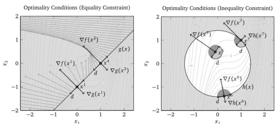
Example 2.4. Consider the nonlinear program of Example 2.3 with just the equality or just the inequality constraint, i.e.,

min x∈R2 f(x) =− x1−1₂ 3 +3₄(x2+1) subject to g(x) =x1−x2−pg=0, (2.5) or min x∈R2 f(x) =− x₁₋1 2 3 +3₄(x2+1) subject to h(x) =x21+x22−2≤0. (2.6)

Problem (2.5)with pg = 1has a local optimal solution x1 = (0,−1) and is globally seen un-bounded. The optimality condition(2.2)is illustrated in Figure 2.2 (left). Note, that the constraint gradient _∇g₍x₎is orthogonal to the constraint g₍x_{) =}0and, thus, possible directions d point in the direction of_{x _∈Rnx |g(x) =0}. In other words, d is tangential to{x∈Rnx |g(x) =0}. For just two points x1 _{and x}4_{= (}_{1, 0}₎_{the condition}_(2.2)_{is satisfied for all directions d. Because}

x4 _{is actually a maximum of} _(2.5)_{, the condition}_(2.2)_{cannot be sufficient. Further note, that}

5_{See Theorem A.14.}

(33)

2.1. Optimality Conditions 13 5 5 5 5 1 1 1 0 0 0 0 −1 −1 −1 −1 −5 − 5 −5 −5 g(x) ∇f(x1) ∇f(x2) ∇g(x1) ∇g(x2₎ d d x1 x4 −2 −1 0 1 2 −2 −1 0 1 2 x1 x2

Optimality Conditions (Equality Constraint)

5 5 5 5 1 1 1 0 0 0 0 −1 − 1 −1 −1 − 5 − 5 −5 −5 h(x) d d d ∇f(x5) ∇f(x6₎ ∇f(x7) ∇h(x6₎ ∇h(x7₎ x5 x6 x7 −2 −1 0 1 2 −2 −1 0 1 2 x1 x2

Optimality Conditions (Inequality Constraint)

Figure 2.2: Geometric interpretation of optimality conditions for Example 2.4. Left: Conditions for one equality

constraint (objective gradients are light gray; gradients and directionsd for which (2.2) is satisfied are black; constraint gradients are scaled by 0.3); Right: Conditions for one inequality constraints (directionsdsatisfying the tangential inequality are contained in the dark gray sectors and those additionally are a descent direction for the objective function in the light gray sectors; constraint gradients are scaled by 0.1).

for these two points, the objective gradient_∇f(x)is parallel or – in other words – proportional

to the constraint gradient_∇g₍x₎, i.e.,_∇f₍x_{) =}₋λ_∇g₍x₎for someλ_∈Rand x∈

x1_,_x4 _.

Problem(2.6) has the local and global optimal solution x6 _≈ ₍_0.277,₋_1.387₎_{. For this point,}

Figure 2.2 (right) reveals the same properties discussed above for problem(2.5). In particular, it holds that_∇f x6

=−ν∇h x6for someν∈R0+. For all other points x there exist descent directions d with ∇h(x)⊤d ≤ 0 if 1 ∈ A(x), i.e., points violating ∇f(x)⊤d ≥ 0, which is

indicated by the light gray sectors around x5 _{and x}7_{in Figure 2.2 (right).}

First-Order Necessary Optimality Conditions

Summarizing the above motivation, inactive inequality constraints can be neglected for the optimality conditions and only active inequality and equality constraints are of interest. These form the boundary of the feasible region_D. The motivation looked for vectors d _∈Rnx with

two properties (cf., Figure 2.2): i. d is tangential to_D.

ii. d is not a descent direction for the objective function f(x).

While property (i) was easy to check for the case of just one constraint (cf., (2.1a) and (2.3)), the union of several constraints to formD requires special care. First, one has to define what it means for a vector to be tangent to the feasible region_Dof a general (NLP).

Definition 2.5 (Tangent Cone). Let_{D ̸}₌_;. A vector d_∈Rnx is called tangent toD at a point x_{∈ D}, if there exist sequencesxk _{⊆ D}_and_{_t

k} ⊆R+ such that lim k→∞x k =x, lim k→∞tk=0, and klim→∞ xk₋_x t_k =d.

(34)

The set of all tangents to_Dat x is called the tangent cone_T_D₍x₎.

It can be shown that the tangent cone _T_D(x) is a closed set (cf., Geiger and Kanzow [84,

Lemma 2.29]). Using it, one can generalize the motivation at the beginning of this section to

formulate a necessary optimality condition.

Theorem 2.6 (Optimality Condition). Let x∗ be a local optimal solution of (NLP). Then,

∇f(x∗)⊤d≥0for all d_{∈ T}_D(x∗).

Proof. See, for example, Fletcher_[68, Lemma 9.2.3_]or Spellucci_[181, Theorem 2.1.1’_]. Unfortunately, the optimality condition of Theorem 2.6 is impractical, since it is difficult to determine the tangent cone_T_D(x∗)in general. Instead, one aims for a condition that resembles

the motivation. Therefore, thelinearized tangent cone is defined and its basic relation to the tangent cone is presented.

Definition 2.7 (Linearized Tangent Cone). For a feasible point x∈ D, the linearized tangent cone is defined as

Tlin(x):=

d_∈Rnx | ∇g(x)⊤d=0and∇hi(x)⊤d≤0,i∈ A(x) . Lemma 2.8. Let x_{∈ D}. Then,_T_D₍x₎_{⊆ T}_lin₍x₎.

Proof. See, for example, Geiger and Kanzow[84, Lemma 2.32]or Nocedal and Wright[151,

Lemma 12.2].

The linearized tangent cone Tlin(x) is also called set of linearized feasible directions in the

literature. Using the first-order approximation _Tlin(x) to the tangent coneTD(x), however,

only makes sense if it captures its main geometric features at the point x. To guarantee this, the constraints have to fulfill some conditions, calledconstraint qualification(CQ). One of the most general is theAbadie constraint qualification, which simply requires the equivalence of the two cones.

Definition 2.9 (Abadie Constraint Qualification (Abadie CQ)). The Abadie constraint qual-ification holds for a point x, if_T_D₍x_{) =}_T_lin₍x₎.

While the Abadie CQ is important in theory, it is highly impractical. Other commonly used con-straint qualifications are thelinear independence constraint qualificationand the Mangasarian-Fromovitz constraint qualification[138], which both imply the Abadie CQ.

Definition 2.10 (Linear Independence Constraint Qualification (LICQ)). The linear inde-pendence constraint qualification holds for a point x, if the gradients _∇g(x) and ∇h_i(x)with

i_{∈ A}₍x₎are linearly independent.

Definition 2.11 (Mangasarian-Fromovitz Constraint Qualification (MFCQ)). The Mangasarian-Fromovitz constraint qualification holds for a point x, if the gradients_∇g(x)are

linearly independent and there exists d _∈Rnx\ {0}such that∇g(x)⊤d =0and∇hi(x)⊤d <0 for i_{∈ A}₍x₎.

(35)

2.1. Optimality Conditions 15

Lemma 2.12. For a feasible point x∈ Dthe following is true: i. If the LICQ is satisfied at x, then the MFCQ is satisfied at x. ii. If the MFCQ is satisfied at x, then the Abadie CQ is satisfies at x.

Proof. See, for example, the proof of Geiger and Kanzow [84, Theorem 2.39 and Theorem

2.41].

For an overview of all the constraint qualifications and their relations, the reader is referred to Peterson[160]. Now assuming for instance the practical LICQ, the optimality condition of

Theorem 2.6 becomes more tractable.

Corollary 2.13 (First-Order Optimality Condition). Let x∗ be a local optimal solution of

(NLP)satisfying the LICQ. Then,_∇f(x∗)⊤d≥0for all d_{∈ T}lin(x∗).

Lagrangian Based First-Order Necessary Optimality Conditions

From a practitioners point of view, there is still one bothersome aspect of the first-order opti-mality condition of Corollary 2.13: The necessary condition_∇f(x∗)⊤d≥0 has to be checked

for all d_{∈ Tlin}₍x∗₎_{. To avoid this, the observation of Example 2.4 – at the optimal solution} _x∗

the gradient_∇f(x∗)was proportional to∇g(x∗)or∇h(x), respectively – is used. To generalize

this, theLagrangian functionis defined.

Definition 2.14 (Lagrangian Function). Letλ_∈Rng andν∈Rnh. The Lagrangian function is defined as

L₍x,λ,ν):= f(x) +λ⊤g(x) +ν⊤h(x)

andλandνare called Lagrangian multipliers or dual variables.

By combining Theorem 2.6 and Farkas Lemma7_{, one ends up at the}_{Karush-Kuhn-Tucker}

con-ditions[126, 131]. Using the Lagrangian function they can be written compactly as follows. Theorem 2.15 (Karush-Kuhn-Tucker (KKT) Conditions). Let x∗be a local optimal solution of

(NLP)satisfying the Abadie CQ. Then, there exist Lagrangian multipliersλ∗∈Rng andν∗∈Rnh,

ν∗_≥0such that

∇xL(x∗,λ∗,ν∗) = ∇f(x∗) +∇g(x∗)λ∗+∇h(x∗)ν∗=0, (2.7a)