Universitat Politècnica de Catalunya
Escola Tècnica Superior d’Enginyeria de Telecomunicació de Barcelona
Signal Theory and Communications Department
A DEGREE THESIS
by David Rodríguez Navarro
Multimodal Deep Learning methods for person
annotation in video sequences
Academic Supervisor: Prof. Josep Ramon Morros Rubió In partial fulfilment of the requirements for the degree in Audiovisual Systems Engineering ___________________________________________________________________ Barcelona June 2017
Multimodal Deep Learning methods for person annotation in video sequences
0.
ABSTRACT
In unsupervised identity recognition in video sequences systems, which is a very active field of research in computer vision, the use of convolutional neural networks (CNN’s) is currently gaining a lot of interest due to the great results that this techniques have been shown in face recognition and verification problems in recent years.
In this thesis, the improvement of a CNN applied for face verification will be made in the context of an unsupervised identity annotation system developed for the MediaEval 2016 task. This improvement will be achieved by training the 2016 CNN architecture with images from the task database, which is now possible since we can use the last version outputs, along with a data augmentation method applied to the previously extracted samples.
In addition, a new multimodal verification system is implemented merging both visual and audio feature vectors. An evaluation of the margin of improvement that these techniques introduce in the whole system will be made, comparing against the State‐of‐the‐Art. Finally some conclusions will be exposed based on the obtained results will be drawn along with some possible future lines of work. Keywords: Deep learning, convolutional neural networks, video annotation, triplet neural network, face identification, face verification.
Multimodal Deep Learning methods for person annotation in video sequences
1.
RESUM
En els sistemes de reconeixement d’identitat no supervisats, el qual és un camp d’investigació molt actiu en la visió per computador, l’ús de xarxes neuronals convolucionals (CNN’s) està rebent molt interès actualment degut als grans resultats que aquestes tècniques están conseguint en tasques de reconeixement i verificació facial els últims anys. En aquesta tesi es realitzarà una millora d’una CNN aplicada a verificació facial en el context d’un sistema d’anotació d’identitat no supervisat, el qual ve ser realitzar per la tasca MediaEval 2016. Aquesta millora serà duta a terme re‐entrenant l’arquitectura neuronal del 2016 amb imatges de la base de dades de la tasca, ara possible degut a que podem utilitzar els resultats del sistema del 2016, a més d’un mètode de data augmentation el qual és aplicat sobre aquestes imatges obtingudes anteriorment.A mes, s’implementarà un nou sistema multimodal de verificació fusionant els vectors de característiques obtinguts per els sistemes de video i audio. També s’evaluaran els marges de millora que introdueixen aquestes tècniques, en comparació amb l’estat de l’art.
Per últim, s’exposen algunes conclusions basades en els resultats obtinguts junt amb posibles noves líneas de treball. Paraules clau: Deep learning, xarxes neuronals convolucionals, anotació de video, xarxes neuronals triplet, identificació facial, verificació facial.
Multimodal Deep Learning methods for person annotation in video sequences
2.
RESUMEN
En los sistemas de reconocimiento de identidad no supervisados, el cual es un campo de investigación muy activo en la visión por computador, el uso de redes neuronales convolucionales (CNN’s) está recibiendo mucho interés actualmente, debido a los grandes resultados que estas técnicas están consiguiendo en tareas de reconocimiento i verificación facial en los últimos años. En esta tesis se realizará una mejora de una CNN aplicada a verificación facial en el contexto de un sistema de anotación de identidad no supervisado, el cual fue realizado para la tarea MediaEval 2016. Esta mejora será llevada a cabo re‐entrenando la arquitectura neuronal de 2016 con imágenes de la base de datos de la tarea, lo cual ahora es posible ya que podemos usar los resultados del sistema del 2016, además de un método de data augmentation el cual se aplicará sobre estas imágenes obtenidas anteriormente.
Además, se implementará un nuevo sistema multimodal de verificación fusionando los vectores de características obtenidos por los sistemas de video y audio. También se evaluaran los margenes de mejora que introducen estas técnicas, en comparación con el estado del arte.
Por último, se exponen algunas conclusiones basadas en los resultados obtenidos junto con posibles líneas de trabajo futuras.
Palabras clave: Deep learning, redes neuronals convolucionales, anotación de video, redes neuronales triplet, identificación facial, verificación facial.
Multimodal Deep Learning methods for person annotation in video sequences
3.
ACKNOWLEDGEMENTS
I would like to show my gratitude to Prof. Josep Ramon Morros, my project supervisor, for his help, support, suggestions and the confidence he placed in me to fulfil this project. His knowledge in video processing and deep learning helped me understanding the details of the covered techniques.
Furthermore, I want to give my thanks for the help given by the technical team in the D5 building, Albert Gil and Josep Pujal, for their backup in technical inquires that I had during the development of the project.
Last, I want to thank my family along with my friends for their encouragement all through this project.
Multimodal Deep Learning methods for person annotation in video sequences
REVISION HISTORY AND APPROVAL RECORD
Revision Date Purpose
0 27/03/2017 Document creation 1 14/04/2017 Document revision 2 15/05/2017 Document revision 3 23/06/2017 Document revision 4 28/06/2017 Document revision 5 29/06/2017 Document revision 6 30/06/2017 Document revision DOCUMENT DISTRIBUTION LIST
Name
David Rodríguez Navarro Josep Ramon Morros Rubió [email protected] [email protected] WRITTEN BY: REVIEWED AND APPROVED BY: Date Date Name David Rodríguez Navarro Position Project author Name Josep Ramon Morros Rubió Position Project supervisor
Multimodal Deep Learning methods for person annotation in video sequences
4.
CONTENTS
1. Introduction 1.1. Project Overview . . . 9 1.2. Requirements and specifications . . . 9 1.3. Work Plan . . . 10 2. State of the art 2.1. Definition of unsupervised video annotation system . . . 11 2.2. Face recognition and verification . . . 12 2.3. Convolutional Neural Networks . . . 12 2.4. CNN architectures for face verification . . . 16 2.5. Multimodal feature vectors . . . 19 3. Methodology and project development 3.1. Systems overview . . . 21 3.2. Database generation . . . 22 3.3. Network training . . . 23 3.4. Verification procedure . . . 26 3.5. Multimodal feature‐level fusion . . . 27 3.6. Evaluation metric: Mean Average Precision . . . 29 4. Experiments and Results 4.1. CNN training . . . 31 4.2. Multimodal fusion . . . 34 5. Conclusions and future development 4.1. Future lines of research . . . 38 BibliographyMultimodal Deep Learning methods for person annotation in video sequences
0.
LIST
OF
FIGURES
1. Different possible casuistry of appearance in videos . . . 11 2. Examples of verificationd and recognition procedures . . . 12 3. Scheme of a basic ConvNet . . . 13 4. Filters from the last convolutional layer from our 2016 VGG‐16 . . . 13 5. How the filter looks at a region from its input and computes its output . . . 14 6. Basic distribution of a CNN hidden layer with its dimensions . . . 14 7. Example of average and max. pooling . . . 15 8. Scheme of a Siamese neural network architecture . . . 17 9. Graphical example of how metric learning affects to its input samples . . . 18 10. Architecture of a generic triplet‐loss CNN . . . 19 11. Block diagram of the structure from the UPC MediaEval submitted system . . . 21 12. Block diagram of the structure from our implemented multimodal system . . . 22 13. Results from applying our data augmentation algorithm . . . 23 14. VGG‐16 main architecture . . . 24 15. Diagram of our triplet‐loss neural network architecture . . . . 25 16. Diagram of the MCB Pooling algorithm . . . 28 17. Tensor Sketch algorithm formalization . . . 28 18. VGG‐16 finetuning error curve from the first dataset (1e‐6 and 1e‐4 decay) . . . 32 19. VGG‐16 finetuning error curve from second dataset (1e‐5 decay) . . . 33 20. VGG‐16 finetuning error curve from third dataset (1e‐5 decay) . . . 33 21. Examples of two name + face recognition errors from our dataset . . . 3422. Two face tracks with a same related name and track assigned to an erroneous name . . . 37
Multimodal Deep Learning methods for person annotation in video sequences
0.
LIST
OF
TABLES
1. Number of parameters to finetune our VGG‐16 architecture . . . 24 2. Summary of all layers from the developed autoencoder . . . 29 3. Generated datasets with its source samples, sizes and number of identities . . . 31 4. Results from applying MAP on the hypothesis generated by our first verification configuration . . . 35 5. Comparison against concatenation and MCB Pooling + PCA reduction with second‐last or last fully connected layer extracted features . . . 36
Multimodal Deep Learning methods for person annotation in video sequences
1
Introduction
This chapter provides a general overview of the project, its main goals and a work plan showing the general project’s organization and deadlines.1.1
Project Overview
Unsupervised identity recognition in video sequences is a difficult issue to deal with due to the lack of labelled data for training the model, since the identities that appear in the video are totally unknown. The use of deep neural networks for this sort of problems is widely extended nowadays because of its robustness when facing non‐seen identities and its considerably fast test execution time.This project is related to previous lines of work followed in the field of unsupervised person annotation in video sequences. Concretely, it continues the Master Thesis Dissertation in Computer Vision made by Gerard Martí Juan [1], where he analysed several convolutional neural network architectures and verification procedures in order to obtain the best face verification performance. The main purpose of this project is to improve the 2016 UPC MediaEval annotation system [2], specifically the triplet neural network face verification stage, as well as implementing a whole new multimodal verification model using combined feature vectors which will contain video and audio information extracted from the shots. Several state of the art techniques will be analysed before proposing new ones in order to have a strong background to start the project with. Also, a possible collaboration with the Speech Processing Group (VEU) will be necessary in order to accomplish the second purpose.
1.2
Requirements and specifications
The project main goals are the following:1. Analysis and improvement of the monomodal annotation system implemented for 2016 MediaEval task.
2. Development of a new multimodal person annotation system, exploring and evaluating different Neural Network (NN) architectures for the verification stage.
3. Evaluate and test the developed techniques performance and compare them to the previously analysed State‐of‐the‐Art techniques. 4. Form a judgment about the system performance and expose some possible improvements and future lines of work.
Multimodal Deep Learning methods for person annotation in video sequences
1.3
Work Plan
The work packages distribution and milestones followed during the project development have remained as the ones presented in the critical review report submitted on 7th May of 2017. In spite of some dilation of certain package deadlines due to problems with the GPI servers, which were non‐operational for maintenance reasons at various times, and problems with the 2016 system (because the API’s of some packages had changed), the milestones were still achieved just in time, as seen in the following graphic:
Multimodal Deep Learning methods for person annotation in video sequences
2
State of the art
This chapter gives an introduction to the concepts of unsupervised annotation systems, Convolutional Neural Network, metric learning and decision/feature‐level fusion for extracted feature vectors.
2.1
Definition of Unsupervised video annotation system
Normally, in a supervised framework, the performance of a video annotation system is as follows: Given a certain video we should be able to determine the presence of a person in every frame, if any, and then determine its identity. In order to accomplish this, a previous person model is built from labelled data. These kinds of systems tend to be multimodal, which means that they exploit the visual and audio features of the video.When we do not have this previously labelled data to train the models we talk about an unsupervised system, because the identities appearing during the video are unknown. This notably increases the difficulty of the problem, which has to be approached in a different way.
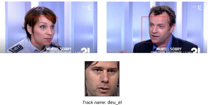
Facial and voice features must be associated with a name (which can be extracted from the speech transcript or from the text overlay, as we can see in figure 1) since we aim to determine the people that appear in the shot and speak at the same time, as explained in the benchmark task [3]. Once we have an identity, we can search through the videos to propagate this detected identities in order to check if it’s appearing somewhere else, which is done by applying a face verification of the non‐identified faces (the ones that are not related to any name) versus the identified ones. This last part is the main focus of our project. Figure 1. Different possible situations of appearing persons. As it can be seen only the appearing and speaking identities must be noted. Image credit: MediaEval [3] From figure 1 we can guess that there is a great variety of different situations that could be given during the video (several people appearing in the same shot, a single non‐speaking person appearing, a person speaking but not appearing, a person appearing but another speaking and not appearing…). All this possible casuistry implies more difficulty when interpreting and combining the multi‐modal information for the tagging task, making the system less accurate.
Multimodal Deep Learning methods for person annotation in video sequences
2.2
Face recognition and verification
As seen in the previous chapter, an unsupervised annotation system consists of a lot of different sub‐systems working together. The focus of this project is on the UPC 2016 MediaEval face verification and recognition part of the whole system, which we aim to improve.
Sometimes these terms are used incorrectly, referring to verification when talking about recognition and backwards, when these terms actually solve different problems or questions. A recognition system answers the following question: Who is this person? This is achieved by comparing a query face to all our available models, and deciding to which one it belongs, which is called 1‐to‐N matching. Otherwise, a verification system aims to answer “Is this person that specific person?” or, more technically, it gives a boolean answer to the comparison between the query face and one model at each time (1‐to‐1 matching). Figure 2. Examples of a verification system 1‐to‐1 (left) and a recognition system 1‐to‐N (right) procedure.
Before neural networks were used, automatic annotation in video sequences was a task that required many complex subsystems working together in a very specific and controlled framework. Some of the most famous systems were the presented by Everingham, M. et al. [4], where frontal face detection and lip movement detection were used along with the video scripts to annotate the appearing and talking persons.
In [5], by Bredin, H. et al., the structure of the presented system is really similar to ours: Each mono‐modal component is processed separately (speaker diarization plus speech‐to text, face detection, tracking and written names on screen) and then a decision‐level fusion is performed. The difference is that any of these stages are performed using deep learning (HoG [6]/LDML [7] or DCT/SVM methods are used for face recognition instead).
2.3
Convolutional Neural Networks
Convolutional neural networks (CNN’s) are a specific type of feed‐forward neural networks, which means that they are made up of neurons with learnable biases and weights, followed by a non‐ linearity. The main difference is that for this kind of networks their inputs are meant to be images, which allows us to make certain assumptions to constrain the architecture, reducing considerably Model 1 Model 1 Model 2 Model N Yes No Pr 1 Pr 2 Pr N
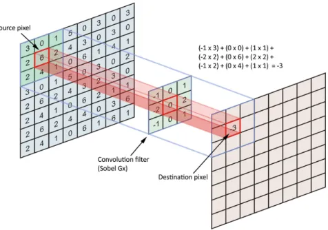
Multimodal Deep Learning methods for person annotation in video sequences the number of parameters in comparison to a regular neural network. Figure 3. Scheme of a basic Convolutional neural network with an input layer, two convolutional layers and a fully connected layer. The relations between the inputs and where each filter is looking at can be seen. This assumption is the following: If a feature is useful to be computed at some spatial position of the image, it probably will be useful at a different position due to statistical invariance (that means that a relevant element can be found at different positions of the same image and remain being the same). This leads us to share the weights and biases of each neuron of the same slice decreasing drastically the number of parameters to train. In figure 4 the filters of the last convolutional layer of the 2016 MediaEval CNN can be seen, where this spatial invariance can be observed as the filter searches for some facial features like eyes, noses, mouths … in different regions of its input. Figure 4. Images of the filters from the last convolutional layer from the CNN of the 2016 UPC task. Image Credit: G.M Dissertation [1] Partially related to the previously said, each neuron is connected only to a local region of the input volume, whose spatial extent is called the receptive field of the neuron (or the filter size). This is made to deal with images as they are high‐dimensional inputs for a regular neural network and also to take advantage of statistical invariance. Since we have this local regions observed by every neuron in a certain position of the layer, with the parameters (weights and biases) shared across all the neurons in the same slice of the layer, we
Multimodal Deep Learning methods for person annotation in video sequences
can think about all the dot products of every neuron with the input region as the convolution of a filter (the weights of the field of view) along the whole image, which is the reason why this architectures are called convolutional neural networks. In figure 5 we can observe an example of how the filter operates in its field of view.
Figure 5. Example of how the filter looks at a region from its input and computes the sum of the element‐wise product of its inner field of view values.
Each hidden layer is formed by three‐dimensional volumes of neurons, where every slice in the volume (all the neurons in the same depth position) share weights and the neurons in the same height and width row look at the same region of the input volume, as we can see in figure 6.
Figure 6. Basic distribution of a hidden layer. The distribution of the three dimensions (height, width, depth in upper image), a closer look of how a same row focuses on the same region with different weights and a basic neuron structure (lower image) are presented. Image credit: http://cs231n.github.io/convolutional‐networks/
Multimodal Deep Learning methods for person annotation in video sequences
This 3‐D disposition involves that at the output of a hidden layer we obtain an activation volume, where every slice is the result of applying a certain filter on its input volume. Also, as in neural networks, at the output of the neurons there is some non‐linear activation function, which in latest CNN’s tends to be a Rectified Linear Unit or ReLU.
The ReLU function basically computes the activation thresholded at zero: , , and it
has become very popular in the last few years because it considerably accelerates the convergence of stochastic gradient descent [8] and it does not involve expensive operations like other activation functions such as sigmoid or tanh.
One of the main problems about ReLU units is that they can be very fragile and can “die” or decay during training, which means that they can end being in an state in which they are inactive for each input, disabling any backward gradient flow, which is usually due to a learning rate set too high. Another usual technique to reduce the number of parameters is adding an extra layer after every convolution layer to reduce the spatial size of the output volumes of it. These layers are called Pooling layers because they join all the elements of its field of view to only one element at its output. There are different criteria on which strategy should be used for pooling the values in the field of view. As we can observe in figure 7, two main techniques are normally used: Max pooling, where the maximum value of the window is taken, and Average pooling, where the average of the values is computed. Nowadays the Max pooling operations is more widely used because, when averaging, we obtain a more “blurred” version of the input and removes more information. Figure 7. Example of how applying an average or max pooling affects to the spatial size reduction.
When the CNN architecture is defined, it has to be trained. This is done inserting train images, computing a loss at the output and then updating the weights and biases in order to reduce the chosen loss, which is called backpropagation. Besides these parameters, which are learnable, every neural network structure has also what is called hyperparameters, non‐trainable and which values are up to the network designer. Some examples of this are the learning rate, the learning decay, momentum, the loss function … In the next chapters we will explain our choices on this hyperparameters when training a CNN and the reason why they are chosen in that way.
Average
Multimodal Deep Learning methods for person annotation in video sequences
With all the techniques previously explained, we aim to have feature maps with its spatial dimensions narrowed, but deeper after each layer. Then, the resulting feature map is flattened in order to connect it to some fully connected layers (FC) which will take care of the final decision or classification, when adding a softmax and some classifier at the end, or will give us a feature vector that characterizes the input. This last utility is the desired when working with face verification, as we will explain in the next section.
2.4
CNN architectures for face verification
The large amount of available data due to the wide flow of multimedia content and the increase of the available computational power are spreading out the use of deep learning and convolutional neural networks to detect, recognize and distinguish between faces, since its results are rapidly improving and leave obsolete the techniques explained at the introduction of this section.As in every type of classification task we need some feature vectors to work with, leading us to the need for a feature extraction procedure. Convolutional neural networks used for regular face recognition work as follows: We input a query image to the neural network and as an output we obtain the probabilities to pertain to every available class, result of applying a softmax layer after the last fully connected layer, turning out that the output at this last FC layer can be used as a good feature vector. As a result, different types of loss functions and architectures to train this CNN’s are being studied in order to obtain the best feature vectors for face recognition and verification. 2.4.1 Single CNN architectures
There are several single CNN architecture configurations, which have proved excellent results in face recognition. Taigman, Y. et al. [9], from Facebook’s AI department, presented a process to build a 3‐D model of the detected faces before feeding the neural network, giving an accuracy of 97,35%, which is really close to the human‐level performance.
A different approach would be the DeepId architecture, presented by Sun Y.et al. [10], where 60 independent CNN’s are trained with different patches of the same picture in order to obtain different high‐level features, which are extracted from the last FC layers and then linearly combined. Another system that provided good results was the named Multi‐view Perceptron, by Zhu Z. et al. [11], a very interesting proposal based in a deep neural network that extracts identity and view features of a single input, being able to generate a multi‐view representation of a face from it.
2.4.2 Metric Learning
As it can be observed, most of the presented techniques of the previous section are based in “simple” neural architectures, where a kind of pre‐processing has been applied to its input images in order to increase its classification or feature extraction robustness.
Although this techniques performance is quite impressive, it has been shown that when working on verification tasks it is more useful to focus in finding a loss function that makes the network learn a
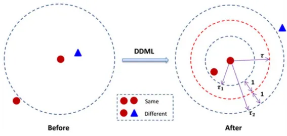
Multimodal Deep Learning methods for person annotation in video sequences distance function over the input samples, which is actually called metric learning [12]. The state of the art verification systems now implement two types of neural network architectures in order to achieve the best distance transformation, which are the following: ● Siamese networks This kind of architecture is based on two identical neural networks, sharing its weights and biases, which receive different inputs. The output of each CNN is taken and joined in a final function, which usually computes the Euclidean distance between the outputs and using different loss functions that suits the requirements in the training stage. A general example of a Siamese architecture is shown in figure 8. Figure 8. Scheme of a Siamese neural network architecture. Using this sort of neural network architecture trained with different pairs of images we can obtain feature vectors which, with a proper distance and loss functions, achieve an interesting property: Given two similar input images, its feature vectors extracted at the end of the neural network will be closer in the output Euclidean space than any non‐similar sample. A clear example of this is the method submitted by Hu, J. et al. [13], which developed a Siamese neural network that minimizes the intra‐class distance relating to a provided minimum threshold and augments the inter‐class distance, making the architecture highly suitable for verification tasks. Before these sorts of architectures were implemented, the used method for increasing the separabilty was the Mahalanobis distance, which is basically based in a linear transformation of the input samples. This worked well but not outstanding, mainly because face images reside in a non‐ linear space, which makes neural networks non‐linearities activations achieve a mapping that suits far better the input samples, obtaining a higher separability, as shown in figure 9.
Multimodal Deep Learning methods for person annotation in video sequences
Figure 9. Graphic example of how applying a distance metric learning method affects to its input samples, reducing the distance between similar samples under a certain threshold t1 and increasing the distances of different samples over t2. Image credit: [13]
As previously discussed, one of the main hyperparameters when training the neuronal network is its loss function as long as it is, apart from other factors, directly related to the weights and biases final values. In Siamese‐loss architectures the most extended loss function is the submitted by Hadsell, Chopra y LeCun [14], called contrastive loss function.
Being Dw the output of the Siamese neural network related to the distance between a pair of
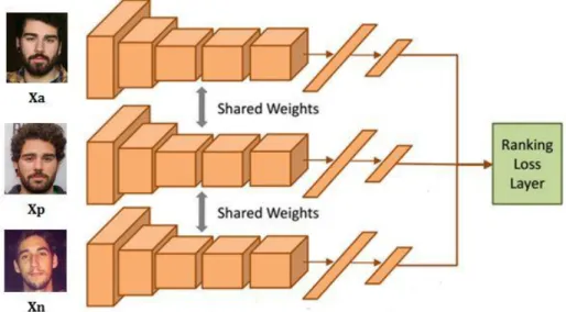
labelled samples x1 and x2 from some pair corpus P… … and Y =1 if both inputs represent the same identity and Y = 0 in the opposite case (different identities), the contrastive loss function is defined as: Where α > 0 is a margin that defines a radius around the outputs of each single network from the Siamese architecture, as can be seen in figure 10. The performance that this loss function presents in a facial verification framework is presented in [15] by the same team, restating the utility of this metric learning architecture. ● Triplet networks As in Siamese networks, triplet‐loss architectures aim of learning a mapping directly from an image to a compact Euclidean space where distances are directly related to faces relationship. The main difference is that in the triplet case we have three identical neural networks, sharing its weights and biases and with its three outputs connected to a common layer that computes the relative similarity for the three images (figure 10). Also three inputs are required in this case, the distribution of which and how are chosen is explained in the following chapter.
Multimodal Deep Learning methods for person annotation in video sequences
Figure 10. Architecture of a generic triplet‐loss convolutional neural network, with its convolutional and FC layers sharing its parameters.
A system that implements this kind of CNN architecture is FaceNet [16] from Google’s Schroff, Kalenichenko and Philbin. Its network is based on GoogLeNet Inception models [17] disposed in a triplet‐loss way, achieving a 99,63% accuracy in Labelled Faces in the Wild (LFW) database and a 95,12% with YoutubeFaces. These results reduced the error rate from the previous state‐of‐the‐art results by 30%.
Another well‐known network is the submitted by Parkhi, M et. al [18], from the Visual Geometry Group of the University of Oxford. First its network is trained for face classification and then finetuned for verification using the triplet‐loss function, achieving accuracy partially similar to FaceNet and DeepFace in LFW dataset, using less data and simpler network architecture.
The loss function training and how neural networks work will be fully explained in the methodology chapter, since this triplet‐loss architecture is the one that we will use in this project so a deeper discussion will be made in further chapters.
2.5
Multimodal feature vectors
So far, all the mentioned methods and systems are based on the modules about extracting and verifying facial features along a video stream but, as explained when we defined the project, our main aim is to identify and annotate the appearing and talking persons on a given video, discarding those people who only appear or speak on it. Considering this constraint it is obvious that we must work with more than one information source, which in our case are audio and video streams. In the 2016 implemented system video and audio sources are separately processed, which results in two labelled groups of tracks. Then, a fusion method based on merging the intersected labelled tracks is applied, with its confidence scores being averaged if both systems had detected the same identity and reducing this by a 0.5 factor otherwise. This kind of multi‐modal methods are called decision‐level fusion systems.
Multimodal Deep Learning methods for person annotation in video sequences margin, it is simple to be aware that fusion method is quite inaccurate. Another way to approach this problem is, once the feature vectors of each source are extracted and labelled and before any classification is performed, create a joint feature vector resulting from mixing both, then carrying out the verification process with this, which seems to make sense since those feature vectors are a fully representation of its identity. This method is called feature‐level fusion. The feature‐level fusion process used to create this mixed feature vectors from different sources, which are called multimodal vectors, is an important area of research in different fields apart from annotation systems. Emotions or sentiments recognition, visual question answering and biometry are areas where this is deeply studied as well.
An example of this is the work submitted by Soujanya et. al [19], where a system for sentiment analysis by classification of multimodal feature vectors composed by audio, visual and textual clues is applied. This is simply made by concatenating its three modalities of feature vectors, creating a single new vector, which is probably the simplest way to fuse some features, being this less accurate than other techniques and infeasible when dealing with long feature vectors. Although its simplicity this technique has been used in several systems [20][21][22][23][24], all of them achieving really good results. Another simple but widely extended method for multimodal pooling is to perform an element‐wise operation, which tends to be a sum or product, between the feature vectors which we aim to fuse. In this way we obtain a joint feature vector with the same size as its inputs, which is an advantage over the concatenating method, although that representation still lacks of expressivity in terms of representing the associations between the original information from the separate vectors. Ideally, what we would like to do is an outer product of both mono‐modal feature vectors, which is called Bilinear pooling [25]. This pooling method computes the outer product between two vectors and learns a linear model that fits better to the problem or question. Unfortunately, this method is usually infeasible due to the high dimensions that this product would present, because of the initial monomodal vectors length. Instead of this, Fukui et. al [26] presented a method called Multimodal Compact Bilinear Pooling, firstly designed for visual question answering, since they had to merge features from images and text from the queries.
What this MCB Pooling operation achieves is a projection of the outer product to a lower dimensional space, evading computing the products itself. This method is explained more extensively in the methodology section.
Multimodal Deep Learning methods for person annotation in video sequences
3
Methodology and project development
In this section we will review in depth the methodology followed during the project, which includes an accurate explanation of the algorithms. First, an overview on the two proposed and tested system will be made. In the second part we will talk about the training procedure of the mentioned network (single neural network training for classification + triplet‐loss training). Then, the verification method used will be described and in the last part we will talk about the procedure followed to implement the multimodal fusion.
3.1
Systems overview
As explained in the introduction chapter this project has two main goals: Improving the MediaEval 2016 submitted system by the UPC, which works with single mono‐modal stages and then fuses the results, and implementing a new multi‐modal system which combines the facial and speech feature vectors before the verification stage. First, our modified 2016 UPC submitted structure and the section that this project focuses is shown in figure 11. Figure 11. Block diagram of the structure from the UPC 2016 MediaEval submitted system.The blocks we focused on for in this part are coloured in red: Data selection block is the implemented system that aims to generate a dataset composed by elements of the video streams delivered for the benchmark, which will be explained in more detail in the following section. The second block is related to finetuning the network that extracts the facial feature vectors with the generated dataset from its previous block. This way it is supposed that this obtained feature
Input video
Text detection Speech segmentation +
diarization OCR
Clustering (video & speech fusion) Facial features
extraction
Facial tracks verification
Decision-level Fusion
Name entity recognition Face detection +
tracking
Data selection & augmentation
Multimodal Deep Learning methods for person annotation in video sequences vectors will suit better our samples domain. In figure 12 we can observe the proposed multimodal verification system. The main difference is that the decision‐level fusion layer is removed and the facial track verification layer becomes the final layer, this time performing the feature‐level fusion and verification. Figure 12. Block diagram of the structure of the 2016 MediaEval submitted by UPC.
3.2
Database generation
In order to make our neural network more suitable for the project framework, a finetuning will be applied to the network pre‐trained model (explained in section 3.3). In [1] G. Martí already performed a finetuning process to the current network architecture using a database composed by a mixture of Labelled Faces in the Wild (LFW) and FaceScrub datasets, which did not produce any significant improvement to it, which was probably caused because this dataset does not help to constrain the network to the provided task images.In this project we take advantage from the fact that we already have a fully implemented annotation system to work with. This makes us able to obtain a ground‐truth related to the MediaEval 2016 datasets to finetune the VGG architecture, which will hopefully make the neural network be closer to the face domain we work with.
3.2.1 Data selection
From 2016 system we can access to all the automatically extracted face tracks and appearing names from the videos used for the task, which we could use in order to create a huge new dataset. The principal issue about using all the images is the different casuistry occurring along the Input video Text detection Face detection + tracking OCR
Clustering (video & speech fusion) Facial features
extraction
Multimodal feature verification (fusion + verification)
Name entity recognition Data selection &
augmentation
Speech segmentation +
Multimodal Deep Learning methods for person annotation in video sequences
videos (figure 1): Many face tracks do not overlap with any name, most of the names overlap with more than one face... And as consequence some criterion has to be applied to select the images that will be part of the database.
This criterion is to use only the names overlapping with a single face track, which will ensure the identity or label of each track. As an aftereffect of this constraint the remaining number of identities is enormously reduced, which can produce a worst convergence of the error when training.
In order to balance this, different database settings could be tested when finetuning the CNN depending on its given results, which will be compared in the experiments section.
3.2.2 Data augmentation
In addition to the problem of selecting which face tracks to use we also have to deal with the fact that, statistically, a big part of the frames from the same video track will be sorely alike, especially in nearby samples. This is something we decided to solve by applying two methods: Frame skips and data augmentation.
Frame skip is basically like a decimating operation applied on the face tracks; picking 1 frame out of x, where this x is a variable we can set before generating the database. Using this we can assert that we have less identical frames in the track, although some will still be very similar. Data augmentation is then applied to the remaining frames in order to increase the intra‐variance of the samples and reduce overfitting.
This data augmentation is carried out by applying arbitrary translations in any direction for a random distance between 0.01 and 0.02 of the full image size and also randomly flipping the face crops from the tracks, being all this done from zero to N times/frame. In figure 13 we can see the results when applying this data augmentation to a certain frame. Figure 13. Results from applying our data augmentation algorithm to the MediaEval database. The rotations and translations can be seen regarding the original crop (left). Data Augmentation
Multimodal Deep Learning methods for person annotation in video sequences
3.3
Network training
3.3.1 VGG‐16 convolutional neural network
Before discussing the training procedure and the loss method itself, it is important to introduce the neural network we are going to work with and the reasons.
In this project the VGG‐D [27], also known as VGG 16 layers, convolutional neural network configuration will be used (figure 14). The main reasons why this architecture was chosen were, first, the good results that it presents in face classification and verification tasks. The other leading reason to choose this network is the current availability of the pre‐trained weights and biases, enabling us to only finetune the network with the desired samples instead of training a full‐neural network, which would be a very time consuming task with our actual resources.
Figure 14. VGG‐16 main architecture.
Before training, we replace the softmax and output layers by others with its corresponding size, depending on the number of identities that our training set has. Then, all the layers of the network are frozen, which means that its weights and biases will not be trained and updated, except for the last convolutional and the last two fully connected layers. This is because it has been demonstrated that the first layers from a CNN detect generic patterns such as contours, texture and colour, but when moving forward the layers it can be observed that the filters become more and more specific to the details related to its training data. This makes feasible training only the last stages of a pre‐ trained network to make it suit our data. VGG‐16 Finetuning Number of parameters Full network 136,362,305 Trainable 124,007,425 Non‐trainable 12,354,880 Table 1. Number of parameters to finetune in our VGG‐16 architecture. The network is initially trained for 20 epochs, with a learning rate of 0.001 caused by the fact that we are performing a finetuning process, where we need fewer epochs to achieve a low loss and the
Multimodal Deep Learning methods for person annotation in video sequences
lower learning rate ensures this to decrease in a smoother way.
3.3.2 Triplet‐loss training
Once the network is finetuned for our samples domain, it needs to be trained for verification purposes. As explained in the state‐of‐the‐art chapter, we want our network to learn to obtain feature vectors with some distance metric related to its inputs similarity. In this project we will use a triplet‐loss architecture.
Training this architecture takes three input images in each cycle called triplets, which are determined as anchor, positive and negative samples (Xa, Xp, Xn in figure 10). Both anchor and positive images must be from the same identity and the negative is a sample from a different identity, no matter which one, in order to ensure that Xa is closer all Xp’s than any Xn sample after training. This distance constraint is expressed the following way:
Where α > 0 is a hyperparameter called learning margin, which function is to regularize the gap between the given distances.
Before starting with the training procedure, the softmax layer of the three single VGG networks is removed since we only need the network to work as a feature vector generator. Instead of this softmax layer, two new layers are added: One computes the l2‐normalization of the result from the last FC layer, and the second is a fully connected layer with no activation function whose purpose is to reduce the feature vector size from 4096 to 1024. The fact of not having activation function implies that this dimension reduction is performed with a simple lineal function. This is shown in figure 15, where the “Input” layer actually refers to the last FC layers of each VGG network. The l2‐normalization and the feature reduction size are computed in the “sequential_1” block and the “Triplet distance” layer computes the final output. Figure 15. Diagram of our triplet‐loss neural network architecture. In order to achieve loss convergence as fast as possible we must select Xn samples that do not fulfil the distance constraint equation, which is called hard‐negative mining. This hard‐negative mining technique also attempts to increase the difficulty of the triplets during the training, selecting combinations of inputs more restrictive in terms of the distance constraint with the aim of obtaining more robust representations at the end.
Multimodal Deep Learning methods for person annotation in video sequences
When a valid triplet has been selected, each image is processed by its corresponding CNN and the Euclidean distance between the anchor and the positive (dan) and the anchor and the negative (dap)
is computed by the final common layer:
Then, as a loss‐function we use what is called margin loss function which is basically the sum, for all the given triplets, of the distance constraint thresholded at zero: This is trained with a stochastic gradient descent method during 10 epochs with a learning rate of 0.25, since we have a new layer, which has to be trained from scratch.
3.4
Verification procedure
Once we have a full triplet‐loss architecture that enables us to extract feature vectors with some metric meaning, we still lack a classifier to evaluate whether a feature vector distance belongs to a same identity or not. For this purpose we will train a Gaussian Naïve Bayes classifier. A GNB classifier assumes that each class distribution (in our case, whether a distance between two face vectors is related to an intra or inter class) is related to a Gaussian distribution, which mean and variance is computed using the feature vectors of all the identities from the training database. When we have each mean and variance, for each new input vector “x” its probability to belong to a certain class “y” is the following:Applying Bayes Theorem we know that: If x independent
Multimodal Deep Learning methods for person annotation in video sequences
Then, using MAP (Maximum A Posteriori) estimation, the class which the distance belongs is the following:
This classifier is really handy to use since it is constantly adapting to the training samples and both train and test time are very fast, as consequence of using a naive assumption of the distribution and a basic classifier.
3.5
Multimodal feature‐level fusion
As stated in the introduction chapter, the second aim of this project is to develop a multimodal version of the already implemented system. This is made by carrying out a feature‐level fusion on the feature vectors coming from the face tracks and the audio block, then applying the verification method previously explained to this new joint features.
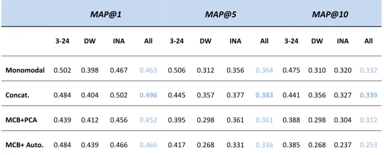
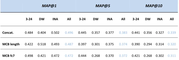
From all the feature fusion methods presented in the previous chapter, in this project we will compare against feature concatenation and multimodal compact bilinear pooling, also known as tensor pooling. The reason why these methods were selected was that concatenation has been the most used fusion technique and its implementation is relatively simple.
3.5.1 Feature concatenation
For the concatenation feature‐level fusion the implemented method is quite simple: The triplet architecture is trained as in the face verification system but this time, for each facial feature triplet its related audio vectors are selected and a concatenation is applied to them. This new feature vectors are introduced into the triplet neural network, which remains as in figure 15, with the concatenation being the first step of the Sequential layer.
As a result we will be obtaining new features with some metric meaning of size 1024, as in the monomodal system, with the difference that these are modelling every identity in a better way since they are composed by two different sources.
3.5.2 Multimodal Compact Bilinear Pooling
As briefly presented in the previous chapter, multimodal compact bilinear pooling (MCB Pooling) aims to compute a lower dimension projection of the outer product between its input vectors, evading computing this product itself. In order to perform this a Count Sketch (CS) algorithm[28] is applied to each vector, projecting this to the desired output space dimension, which in our case has to be higher than the input dimension, seeming unreasonable at first since we aim to reduce the output dimensionality. The key is that the outer product will remain the same size as the chosen when generating the Count Sketch vectors, being this size smaller than what would result from multiplying the original vectors, as we will demonstrate later in the results chapter.
Multimodal Deep Learning methods for person annotation in video sequences
Instead of computing the outer product of the original vectors and applying Count Sketch to the result, which would take much computational power, this count sketch vector is proven to be the same as computing the convolution of the count sketches of its original inputs, as shown in [29]. Likewise, applying the convolution theorem we know that a convolution can be computed as , where ‘∙’ is an element‐wise product. All this is procedures are shown in figure 16. Figure 16. Diagram of the MCB Pooling algorithm. Image credit: [26] This method had to be entirely programed due to the lack of modules on Keras, since this is a very new feature‐level fusion method, following the Tensor Sketch algorithm proposed in [29], which is also shown in figure 17. Figure 17. Tensor Sketch algorithm formalization. Image credit: [26]
Although MCB Pooling algorithm reduces the dimensionality of the resulting multimodal vector, this tends to be still difficult to handle because of its size, especially in our application where these vectors have to be introduced in a triplet‐loss neural network, increasing the number of trainable parameters in an unfeasible way.
Multimodal Deep Learning methods for person annotation in video sequences
In order to avoid that situation we trained a Principal Component Analysis (PCA) [30] and an autoencoder [31] dimensionality reduction model using a set formed by 6093 joint feature vectors, which were obtained by computing the mean of the features from all tracks with a related audio feature, then applying our MCB Pooling algorithm with a resulting vector size of 16k.
The reason why we opted for implementing two dimensionality reductions methods is that, although autoencoders achieve better reduction when they are properly trained, our training data is limited and the amount of parameters to train one like ours are numerous, as it can be seen in table 2.
Autoencoder architecture
Layer Type Output Shape Num. Parameters
input_1 (InputLayer) ( , 16000) 0 dense_1 (Dense) ( , 8192) 131080192 dense_2 (Dense) ( , 4096) 33558528 dense_3 (Dense) ( , 4096) 16781312 dense_4 (Dense) ( , 8192) 33562624 dense_5 (Dense) ( , 16000) 131088000 Total Parameters 346,070,656 Table 2. Summary of all layers from the developed autoencoder for the output from MCB Pooling. This PCA/autoencoder will reduce our multimodal vectors from 16k to 4096, which makes us able to train a triplet‐loss network just as in the previous two methods since its input vector size is the same.
3.6
Evaluation metric: Mean Average Precision
Normally, for classification applications, we rely on performance metrics such as precision, recall, f‐ score and accuracy to know how well our system is working. Since ours an information retrieval task, the evaluation metric we will rely on is the called Mean Average Precision (MAP), which basically computes precision for systems that return a ranked sequence of elements, where the position of its elements is also meaningful.Multimodal Deep Learning methods for person annotation in video sequences
An Average Precision (AP) evaluation for a given query “q” is computed as follows:
Where P(i) is the precision or percentage of correct retrievals among first i recommendations, n is the number of given predictions and m is the number of relevant predictions. Then, Mean Average Precision consists on computing the mean value of Average Precisions for a set of given queries Q: In order to ensure that participants provide proper evidences for each query, a modified version of the MAP evaluation is used. This metric is called evidence‐weighted mean average precision:
Where C(q) is the “correctness” of each proposed evidence when nq, the hypothesized person
name, is close enough to the query q, which is computed by its Levenshtein distance ρq:
Multimodal Deep Learning methods for person annotation in video sequences
4
Experiments and Results
In this section the reasoning between the experiments, its variations due to its results and the differences between the methods described in the previous section are explained. The experiments from the monomodal system will determine the best CNN finetuning method, which will be also used by the multimodal system in case that it achieves good results. Then, the feature‐level fusion methods will be tested in order to observe if any improvement is made in relation to the monomodal system.
4.1
CNN training
As we stated in the methodology chapter, the VGG‐16 CNN (chapter 3) is finetuned using a new database made‐up by images from the MediaEval corpus. Since we created different variations of this, several executions with different parameters were made in order to find the one that suits better our requirements and, also, a comparison against the finetuning made in the 2016 task will be made in search for any improvement.
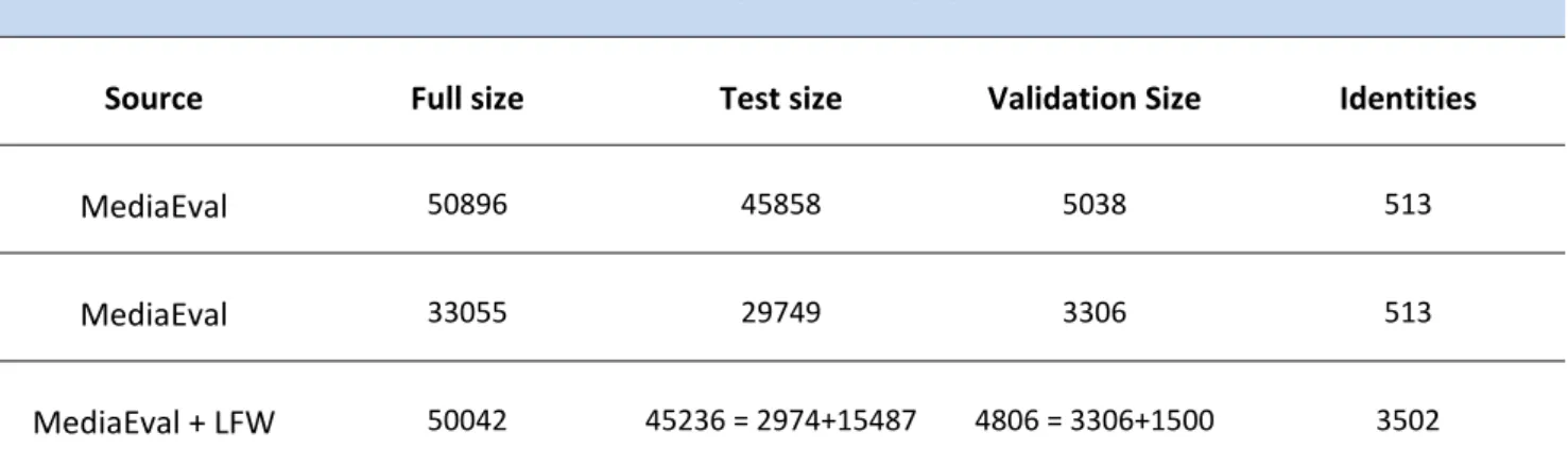
Database Distributions
Source Full size Test size Validation Size Identities
MediaEval 50896 45858 5038 513
MediaEval 33055 29749 3306 513
MediaEval + LFW 50042 45236 = 2974+15487 4806 = 3306+1500 3502
Table 3. Generated datasets with its precedence samples, sizes and number of identities.
The first execution was made using the database from 2016 task [1] in order to have some guide mark when applying finetuning with our own database and, more important, to check if our framework was properly configured. This was made by training over 20 epochs with a learning rate of 0.0001, a learning rate decay of 1e‐6/epoch and momentum of 0.9, obtaining an error similar to the one shown in [1]. Many parts of the 2016 base code had to be corrected and updated as the Keras API did change since 2016. However, these changes do not affect the results.
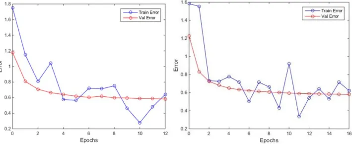
Once the framework and the database generation algorithm were properly working, a new training was performed, this time using the 1st Database from table 3. Since every execution with 20 epochs takes from 2 to 4 days, depending on how busy the server is as that moment, these first executions were made only for 12 epochs and the same parameters as the 2016 finetuning, with the aim of following the evolution of the error first.
Multimodal Deep Learning methods for person annotation in video sequences
learning rate decay of 1e‐6 and 1e‐4, which was made because we expected the learning rate to be initially too high.
Figure 18. VGG‐16 finetuning error curve from the first dataset with 1e‐6 decay (left) and 1e‐4 decay (right).
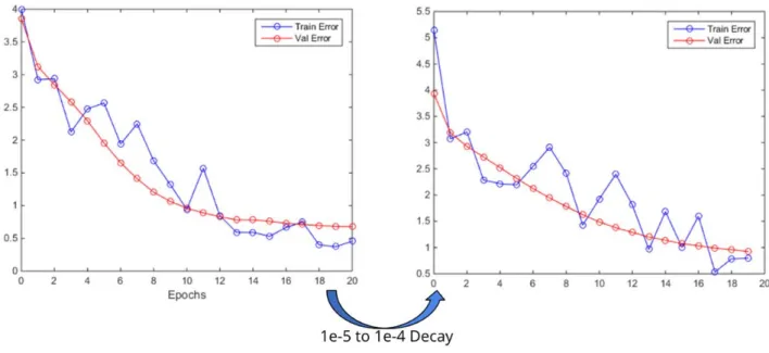
As it can be observed above, with a learning rate decay of 1e‐6, the unevenness of the training error are equally present during all training in both graphics, manifesting that the learning rate might be too high. Increasing the decay to 1e‐4 we can see that for the first epochs the loss curve is a bit smoother in comparison to a lower decay, although its tendency is quite peaked (even 2016 finetuning presented this peaks during training). By the shape of the validation curve it can be said that the learning rate is still too high, since it seem to rapidly converge to a value close to 0.6. A bit of overfitting can be also seen as the training loss is lower than the validation loss in some periods, which could be due to the big amount of images per identity versus 2016 database. Because of these results we decided to create a reduced version of this database, in order to test if having so many similar images per identity, despite the applied methods to augment intra class variance, was the origin of these bad results when training the network. The size and distribution of this database can be found on the second row from table 3. This time the network was trained during 10 epochs with a learning rate decay of 1e‐5, as we observed in the last execution the difference with 1e‐6 was not that significant, and it is also better for learning rate to tend to be a bit lower than too high. The obtained loss is shown in figure 19:
Multimodal Deep Learning methods for person annotation in video sequences
Figure 19. VGG‐16 finetuning error curve from the second dataset (decay: 1e‐5, epochs: 10).
This execution made visible what we already thought: That the abruptness of the last training loss curve was due to an excess of images per identity, having only 513 of them and the same number of images as in 2016 training. Even so, the loss value converges at 0.589, similarly to all the previous executions while 2016 finetuning converged around 0.2, which can be caused by having less samples and identities.
Taking this into account we decided to create another database made of the previously tested dataset merged with some samples from LFW database (third row from table 3). The purpose of this joint database is having our neural network still adapt to our MediaEval samples while providing enough different identities to avoid overfitting. This time we trained the network during 20 epochs to observe the loss convergence, its value and the possibility of overfitting. The obtained error is shown in figure 20: