Applicability of Transient Electromagnetic Fast Forward Modeling
Algorithm with Small Loop
Jian Chen, Fuxue Yan, Yishu Sun, and Yang Zhang*
Abstract—In the forward modeling of the transient electromagnetic (TEM) method, a frequency-domain solution is usually obtained first, and the solution in the time frequency-domain is then calculated by a frequency-time transformation. At present, the three main fast frequency-time transformation methods are the Guptasarma algorithm, the sine and cosine numerical filtering algorithms, and the Gaver-Stehfest (G-S) algorithm. In recent years, with the increasing demand for fine detection at shallow depths, the small-loop TEM method has undergone rapid development. It is therefore important to evaluate whether the traditional forward modeling approaches can be directly applied to the small-loop method. In this paper, the principles of the three forward modeling methods and their limitations when being applied to the small-loop TEM method are discussed. Through a comparison with the analytical solution for a uniform half-space, we demonstrate that the accuracy of forward numerical calculation is affected by loop size and earth resistivity. When the Guptasarma, G-S, and cosine numerical filtering algorithms are used for small-loop TEM forward calculation, the overall calculation error becomes non-negligible, whereas the sine numerical filtering algorithm retains a high calculation accuracy. By studying the response of the frequency-domain solution, we analyze the cause of the error in the forward calculation. Generally, the sine numerical filtering algorithm is the most suitable method for fast and high-precision small-loop TEM forward modeling. The results obtained here should provide a foundation for high-precision forward modeling and inversion of the small-loop TEM method.
1. INTRODUCTION
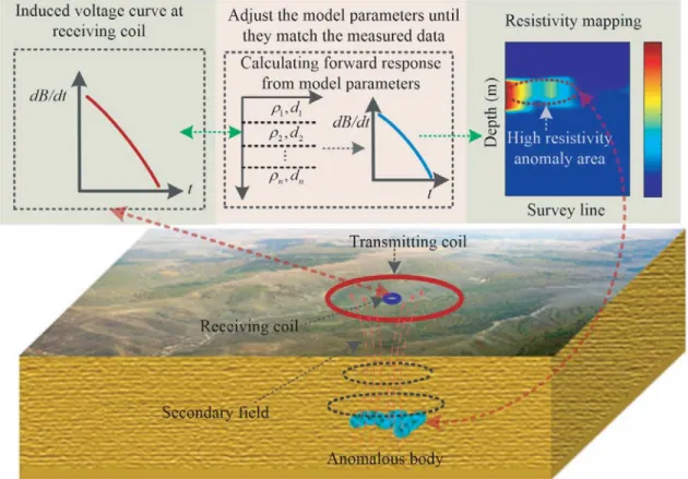
The transient electromagnetic (TEM) method is a rapidly developing noninvasive geophysical exploration technique that is widely used in geological mapping and in exploration of mineral and water resources owing to its good ability to penetrate high-resistivity strata and its high sensitivity to anomaly detection. As shown in Fig. 1, TEM is a method of using an ungrounded loop to emit a pulsed magnetic field to the ground. After the transmitting current is turned off, the secondary eddy current field is obtained by the receiving coil. High-precision forward modeling is essential for TEM data interpretation. Owing to the complexity of two- and three-dimensional forward modeling theory and the huge amount of calculations required [1], the more mature one-dimensional layered model forward modeling method is still widely used. Given that the forward analytical expression involves a Bessel function, the frequency-domain solution is generally obtained by Hankel transformation, and the time-domain solution is then calculated using frequency-time transformation [2, 3]. The most widely used fast frequency-time transformation methods at present are the Gaver-Stehfest (G-S) algorithm, the Guptasarma algorithm, and the sine and cosine numerical filtering algorithms.
Knight and Raiche [4] were the first to use the G-S algorithm to convert a frequency response to a time response in a two-layer geoelectric model, which facilitated the development of forward calculations
Received 16 July 2020, Accepted 14 November 2020, Scheduled 18 November 2020
* Corresponding author: Yang Zhang ([email protected]).
Figure 1. Principle of TEM detection and schematic diagram of forward modeling and inversion interpretation.
in the TEM method. Raiche [5] then applied the G-S algorithm to polygonal loops to obtain a time-domain electromagnetic solution. To solve the efficiency problem caused by a large number of sampling times, Luo and Chang [6] further improved the operating speed of the G-S algorithm using the delay theorem for the Laplace transform. The G-S algorithm has few filtering coefficients and a fast calculation speed, and its calculation accuracy is closely related to the word length of the computer. The greater the word length is, the higher the accuracy is, so the algorithm requires a higher computer performance [7]. Kaufman and Keller [8] first applied the sine and cosine transform algorithms to one-dimensional forward calculations in the TEM method. There are various ways to realize the sine and cosine transforms, such as the Feron algorithm, the broken-line approximation algorithm, and the numerical filtering algorithm. The Feron algorithm requires a large number of calculations, and in the broken-line approximation algorithm, the integration step is difficult to control, and the calculation speed is slow, whereas the numerical filtering algorithm can ensure the accuracy of calculation and greatly improves the speed of operation [9]. The Guptasarma algorithm is a linear filter algorithm proposed by Guptasarma [10] for calculating the time-domain induced polarization response from the frequency domain. The algorithm is suitable for the case where the two extremes of the frequency variables have real asymptotic values, and the amplitude decreases monotonically from low frequency to high frequency. In this algorithm, only 21 filter coefficients are used, so the calculation is fast. In the calculation of the TEM response [11], the accuracy is higher at early times and lower at late times.
The classical TEM forward modeling theory is based on a large-loop source. In recent years, with the increasing demand for exploration of urban underground spaces, tunnels, and mountain disasters, there has been a rapid growth in the use of small-loop TEM systems [12–14]. In this paper, to evaluate the applicability of the traditional forward method for small coils, three different fast forward modeling methods are discussed in detail in the context of their application to small loops. The advantages and limitations of the three methods are revealed by comparing them with analytical solutions for a uniform half-space.
2. FORWARD MODELING THEORY
In this section, we briefly introduce the calculation of the domain solution and the frequency-time conversion method in TEM forward modeling theory, and we present the related core calculation formula. Full details can be found in the references cited.
2.1. Hankel Transform
In electromagnetic sounding theory, for layered earth, the transient electromagnetic field responseV(t) of the central loop device under excitation by a step current is given by [20]
V(t) = −2qμ0 π ∞ 0 Re[Hz(ω)] cos(ωt) dω = 2qμ0 π ∞ 0 Im[Hz(ω)] sin(ωt) dω, (1) where Hz(ω) =I0r ∞ 0 Z(ω, λ)J1(rλ) dλ (2)
is the electromagnetic frequency-domain solution,Z(ω, λ) the transfer function of the layered earth [21], J1 the first-order Bessel function of the first kind, I0 the transmitting current, r the radius of the transmitting coil, μ0 the vacuum permeability, and q the equivalent receiving area. In a horizontal layered medium, the forward formula for transient electromagnetic sounding of a loop source is expressed as a double integral. The inner layer is a Hankel-type integral with a Bessel function of the first kind, and the outer layer is a sine or cosine integral. In the integral formula, since the Bessel function decreases slowly with the independent variable, the solution for layered earth can be obtained only through a numerical calculation method. At present, the high-precision linear numerical filtering formula proposed by Guptasarma and Singh [16] is generally used to calculate the frequency-domain response. The principle of the calculation is as follows:
Hz(ω) = ∞ 0 F(ω, λ)J1(rλ) dλ = 1 r n i=1 F(ω, λi)Ki, F(ω, λi) =I0rZ(ω, λi), λi= (1/r)×10[a+(i−1)s], i= 1,2, . . . , n, (3)
whereF(ω, λi) is the objective function to be converted; the shiftadetermines the starting point of the sampling input function; the sampling intervalsspecifies the interval of the remaining sampling;λiis the position of the sampling point; and Ki is the Hankel transform of the numerical filtering coefficients, whose values are given in [16]. The accuracy of numerical calculation depends on the length of the integration interval n. Generally, the larger the value of n is, the slower the calculation speed is but the higher the accuracy is. In this study, a 140-point Hankel J1 transform is used to obtain the TEM frequency response.
2.2. G-S Algorithm
The G-S algorithm belongs to a class of probability transformation algorithms that involve purely real number operations. It requires only calculation of the s value of the Laplace transform, so its calculation speed is fast. The main idea is to use the basic integral properties of a special function (the kernel function) to connect the function to be solved and the integral of its product with the kernel function, thereby transforming the function to be solved from the frequency domain to the time domain. The core expression of the calculation is as follows [4, 17]:
fGS(t) = ln 2 t N m=1 Wmfω mln 2t , (4)
where Wm = (−1)m+N/2 min(m,N/2) k=[(m+1)/2] kN/2(2k)! (N/2−k)!k!(k−1)!(m−k)!(2k−m)! (5) is the G-S filtering coefficient, fω the response function in the frequency domain to be converted, [(m+ 1)/2] the integer part of (m + 1)/2, and N a positive integer determined by the number of computer bits, which is usually taken from the set{8, 10, 12, 14}. In this study,N is taken as 12. The expression for the time-domain TEM response can be obtained by Gaver and Stehfest’s inverse Laplace transform: VGS(t) =−qμ0ln 2 t N m=1 Hz mln 2t Wm. (6)
Using Eq. (3), it can be deduced that the frequency domain responseHz in Eq. (6) satisfies Hz mln 2 t = 1 r n i=1 F mln 2 t , λi Ki. (7) 2.3. Guptasarma Algorithm
The Guptasarma algorithm can convert the voltage response of an impedance model in the frequency domain that involves a fractional power of the complex frequency variable, such as the Cole-Cole model, to the voltage response under step-current excitation. The specific conversion method is as follows [10]:
fGup(t) = R0− 21 r=1 ϕr Re[R(ωr)], (8) ωr = 10ar−log10t, (9)
where R(ωr) is the frequency-domain impedance of the polarization model, R0 the zero-frequency impedance, ϕr the linear filtering coefficient, and ar the position value, whose specific value can be found in [10]. The filter is applicable to complex impedances with real asymptotic values at the two extremes of the frequency variable for which the amplitude decreases monotonically from low frequency to high frequency. For the TEM field, both the magnetic field response and electric field response have real asymptotic values at the two extremes of the frequency variable, and the amplitude basically shows a monotonic downward trend. Therefore, the linear filtering method can be used for frequency-time conversion of the electromagnetic response [11]. In the forward calculation in the TEM method,R0= 0, and Eq. (8) can be converted to
VGup(t) =−qμ0 21
r=1
ϕrRe[Hz(ωr)]. (10)
2.4. Sine and Cosine Numerical Filtering Algorithms
Sine and cosine transforms are special cases of the Hankel transform, and the associated numerical filtering algorithms can be quickly obtained by using the familiar Hankel transform theory. The main difference between the sine and cosine transforms is that the kernel functions used are the virtual component and the real component of the vertical magnetic field, respectively. The Bessel functions and the sine and cosine functions are related as follows [18]:
J1/2(z) = 2 πz sinz, J−1/2(z) = 2 πz cosz. (11)
The numerical filtering algorithm for the sine and cosine transforms can be deduced as fsin(t) = 1 t π 2 +∞ n=−∞ fω enΔ t csin(nΔ), (12)
fcos(t) = 1 t π 2 +∞ n=−∞ fω enΔ t ccos(nΔ), (13)
where fω is the response function in the frequency domain that is to be converted; Δ is the sampling interval; csin(nΔ) and ccos(nΔ) are the numerical filtering coefficients of the sine and cosine transformations, respectively, and the sine and cosine integrals of the voltage response induced in the central loop device have the forms given in Eq. (1). The numerical filtering forms can be obtained by substituting the above expressions:
Vsin(t) = 2qμ0 tπ π 2 +∞ n=−∞ Im Hz enΔ t csin(nΔ), (14) Vcos(t) = 2qμ0 tπ π 2 +∞ n=−∞ Re Hz enΔ t ccos(nΔ). (15)
In actual calculations, n takes only a limited number of values: the range is generally from −200 to 200. The more filter coefficients are used, the slower the calculation speed is, but the higher the calculation accuracy is. Generally, for the same type of function, the optimum number of filtering coefficients should be determined by experiment [18]. Provided that the calculation accuracy is ensured, the calculation speed should be increased as much as possible. In this study, Δ = ln(10)/10 andn=−59 to 100.
3. COMPARISON OF FORWARD MODELING RESULTS
For the TEM method, an analytical solution is available for the electromagnetic field in the uniform half-space model, and this is not constrained by the coil size, so it can be used as a theoretical reference to evaluate the accuracy of other layered geological forward modeling methods. The analytical expression for the TEM field-induced voltage response of a central loop device in a uniform half-space is [19]
V(t) = 3qI0ρ μ0r3 φ(u)− 2 π u 1 +u 2 3 e−u2/2 , (16)
where u = rμ0/2ρt, φ(u) = 2/π0ue−x2/2dx (probability integral), r is the radius of the transmitting loop (the square loop side length a and circular loop radius r satisfy r = a/√π), and ρ is the resistivity of the uniform half-space. To compare the characteristics and applicability of three different forward modeling methods for large and small loops, this study simulates a large transmitting loop with side length 100 m and a small transmitting loop with side length 5 m. The half-space resistivity is set as 100 Ω·m and the transmitting current as 10 A, and the receiving equivalent area is 10 m2 (the receiving area is mainly realized by increasing the number of receiving turns, and its size is small enough relative to the transmitting coil). The calculation time range is [10−7,10−2], and 30 points of data are sampled according to logarithmic equal intervals. It is worth mentioning that for the small-loop TEM method, data within 1 ms can be regarded as a high-SNR data segment. The calculation results are compared with the uniform half-space analytical solution. In addition, to provide an objective and quantitative evaluation standard for the accuracy and calculation speed of the forward modeling method, the average running time and error of a single forward modeling are defined as
Time = m i=1 Timei m , (17) Error = n i=1 |Forwardi−Analytici| Analytici n ×100% (18)
where Timeiis the duration of one forward modeling,mthe number of forward modelings, Forwardi the ith-channel response value in the forward calculation results, Analytici the ith-channel response value corresponding to the analytical solution, and n the total number of channels. In this study, m = 50 and n= 30.
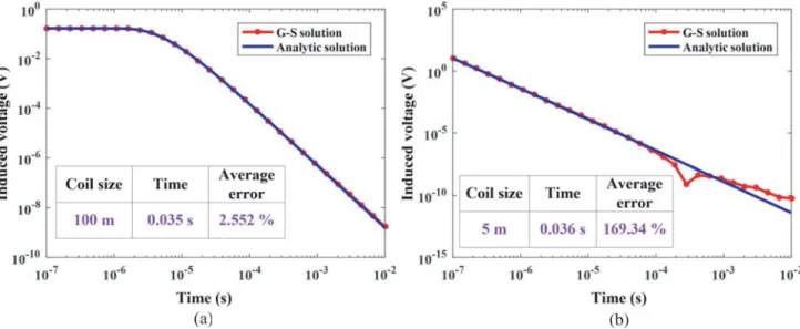
3.1. Results of G-S Algorithm
The forward calculation results obtained with the G-S algorithm are illustrated in Fig. 2. When the algorithm is applied to large-loop TEM forward modeling, the calculation speed and accuracy are relatively high; the calculation error is mainly concentrated at late times; the overall average calculation error is less than 3%; so this algorithm is widely used in large-loop source forward modeling. However, when it is applied to the small loop, the average error of the overall calculation increases by nearly 80 times. At late times, there is a large fluctuation, with negative values appearing (in the figure, all of the data are processed using the absolute value). Only at early times, the coincidence degree is high. Taking account of the fact that the effective data time length can reach the order of milliseconds in actual TEM field detection, the applicability of this method in the small-loop case is severely limited.
(b)
Figure 2. Forward modeling results of the G-S algorithm: (a) large-loop TEM; (b) small-loop TEM (the negative parts of the data are processed using the absolute value).
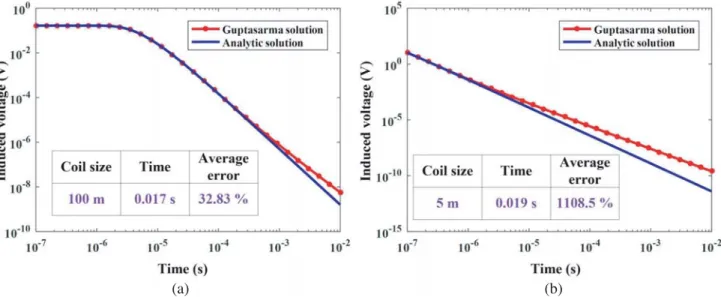
3.2. Results of Guptasarma Algorithm
The calculation results obtained with the Guptasarma algorithm are shown in Fig. 3, from which it can be seen that the calculation speed is twice as fast as that of the G-S algorithm. Because only the real part of the frequency-domain solution is used in frequency-time conversion, the late-time conversion accuracy is relatively low, and the overall average error is large. Fortunately, this method has high accuracy in the [10−7,10−3] time period, and it can realize the most rapid forward modeling, which is in line with actual engineering needs, so it is widely applied to the large-loop TEM method. However, when being applied to the small-loop method, although there is no negative fluctuation similar to that occurring with the G-S algorithm, the overall calculation error becomes larger. The time period for which accurate calculations are possible is greatly reduced, and also the average error is over 1000%, which is far from meeting actual engineering measurement requirements. Therefore, this method is unsuitable for application to the small-loop TEM method.
(a) (b)
Figure 3. Forward modeling results of the Guptasarma algorithm: (a) large-loop TEM; (b) small-loop TEM.
3.3. Results of Sine and Cosine Numerical Filtering Algorithms
The cosine numerical filtering algorithm uses the real component of the magnetic field, which provides high calculation accuracy at early times, although a fluctuation will occur at late times (Fig. 4). This fluctuation phenomenon will appear earlier and more strongly in small-loop TEM. The sine numerical filtering algorithm uses the imaginary component of the magnetic field. Its calculation accuracy is nearly 50 times higher than that of the G-S algorithm, and the overall average error is less than 0.1% (Fig. 5). However, the calculation speed of this method is the slowest among the three types of numerical algorithm, with its calculation time about three times as long as that of the G-S algorithm. However, compared with the broken-line approximation method and the Feron algorithm (which usually take several seconds for one forward modeling), its calculation speed is still considerable. When the algorithm is applied to a small coil, its operation speed is basically unaffected. Although the calculation
(a) (b)
Figure 4. Forward modeling results of the cosine numerical filtering algorithm: (a) large-loop TEM; (b) small-loop TEM (the negative parts of the data are processed using the absolute value).
(a) (b)
Figure 5. Forward modeling results of the sine numerical filtering algorithm: (a) large-loop TEM; (b) small-loop TEM.
error becomes larger, the accuracy remains high and is equivalent to that of the G-S algorithm for large-loop forward modeling.
4. DISCUSSION
4.1. Relationship between Frequency-Domain Solution Response and Loop Size
The relationship between the vertical magnetic field and the frequency received by the uniform half-space central loop device is as follows [15]:
Hz(ω) =−kI02 1r3
3−3 + 3k1r+k21r2e−k1r, k2
1 =−iσωμ0, (19)
wherek1 is the underground wave number in the uniform half-space,σ the conductivity of the uniform half-space, ω the circular frequency (ω and frequencyf satisfy the conversion relationf =ω/2π), and r the radius of the transmitting loop. The square loop side lengtha and circular loop radiusr satisfy r =a/√π. The size of the loop directly affects the solution for the frequency-domain response. With a small loop, the sampling position in the frequency response calculation is increased owing to the reduction in the offset distance, which makes the sampling interval of the formation transfer function larger. To evaluate the influence of the small loop on the frequency solution in an intuitive manner, the frequency is calculated analytically for side length of 100 m and 5 m. The transmitting current is 1 A; the half-space resistivity is 100 Ω·m; and the number of frequency points is 300. In the case of a large central loop (Fig. 6(a)), the real part of the magnetic field oscillates in the high-frequency band, but it is very stable in the low-frequency band, while the imaginary part of the magnetic field is not completely stable, but it is generally smooth. In the high frequency region, the interaction between the induced eddy current fields in the ground becomes non-negligible, which leads to the generation of oscillation signals. When the coil size is reduced (Fig. 6(b)), the response in the low-frequency band is extended to the high-frequency band. It can be seen from the calculation errors of the three numerical forward modeling methods (Fig. 7) that compared with the case of a large loop, the overall calculation error for a small loop will shift to early times, and consequently the calculation error will appear earlier in the small-loop TEM method. For the Guptasarma and cosine transform algorithms, which use the real part of the magnetic field, the late-time error caused by high-frequency oscillations cannot be ignored in the case of a small loop. By contrast, the sine numerical filtering algorithm uses the relatively smooth imaginary component of the magnetic field, which provides good calculation accuracy and stability.
(a) (b)
Figure 6. Variation of the vertical magnetic field with frequency at the center of the transmitting loop: (a) large-loop TEM; (b) small-loop TEM.
(a) (b)
Figure 7. Comparison of calculation errors of the three fast forward modeling methods: (a) large-loop TEM; (b) small-loop TEM.
4.2. Influence of Earth Resistivity
For the small-loop sine numerical filtering algorithm, we study the calculation accuracy and speed for different values of the earth resistivity. The results are shown in Fig. 8. With increasing resistivity, the forward calculation speed slows down slightly, and the calculation error gradually increases, especially in the time period [10−3,10−2], and the relative error fluctuates strongly. The reduced accuracy of forward calculation at late times will lead to problems in the interpretation of data on deep high-resistance bodies. In actual field measurements, especially in complex environments such as cities and tunnels, the TEM signal in this period is often contaminated by noise, and although this does not affect the applicability of the sine transform algorithm to the small-loop TEM method, it implies that if the appropriate forward calculation method is not chosen, the error in early-time calculation results may become large owing to the presence of underground high-resistivity bodies.
Figure 8. Influence of resistivity on the calculation error of the sine numerical filtering algorithm.
5. CONCLUSION
This paper has described the basic principles of three classical fast forward modeling methods based on the large-loop TEM method: the G-S algorithm, the Guptasarma algorithm, and the sine and cosine transform algorithms. Through a comparison with the uniform half-space analytical solution, we have demonstrated that the accuracy of forward numerical calculation is affected by loop size and earth resistivity. The smaller the transmit-receive distance is, the larger the sampling interval is in the frequency calculation. This makes the low-frequency response appear earlier in the numerical calculation results, as a consequence of which the overall calculation error shifts to early times, and the calculation error appears earlier in the small-loop TEM method. Furthermore, the real part of the numerical solution in the frequency domain oscillates in the high-frequency band, and therefore the errors in the Guptasarma algorithm, the G-S algorithm, and the cosine transform algorithm cannot be ignored when they are used in the small-loop forward calculation. The sine numerical filtering algorithm uses the relatively smooth imaginary component in the frequency-domain solution, which provides high overall calculation accuracy, with only slight oscillations occurring at late times. For subsurface low-resistivity structures, the calculation accuracy and speed of this algorithm are further improved, which is consistent with the high detection sensitivity of the TEM method for low-resistance anomalies. Thus, at present, the sine numerical filtering algorithm is the most suitable approach for fast and high-precision forward modeling in the small-loop TEM method.
ACKNOWLEDGMENT
This research was supported by National Natural Science Foundation of China (Grant Nos. 41827803, 61903151), Postdoctoral Science Foundation of China (Grant Nos. 2019M651205), Graduate Innovation Fund of Jilin University and the Engineering Research Center of Geothermal Resources Development Technology and Equipment, Ministry of Education, Jilin University.
REFERENCES
1. Auken, E., T. Boesen, and A. V. Christiansen, “A review of airborne electromagnetic methods with focus on geotechnical and hydrological applications from 2007 to 2017,” Advances in Geophysics, Vol. 58, 47–93, 2017.
2. Nabighian, M. N., “Quasi-static transient response of a conducting half-space: An approximate representation,” Geophysics, Vol. 44, No. 10, 1700, 1979.
3. Ali, M. T., E. Slob, and W. Mulder, “Quasi-analytical method for frequency-to-time conversion in CSEM applications,” Geophysics, Vol. 77, No. 5, 357–363, 2012.
4. Knight, J. H. and A. P. Raiche, “Transient electromagnetic calculations using the Gaver Stehfest inverse Laplace transform method,” Geophysics, Vol. 47, No. 1, 47–50, 1982.
5. Raiche, A. P., “Transient electromagnetic field computations for polygonal loops on layered earths,”
Geophysics, Vol. 52, No. 6, 785–793, 1987.
6. Luo, Y. Z. and Y. J. Chang, “A rapid algorithm for G-S transform,”Chinese Journal of Geophysics, Vol. 43, No. 5, 724–730, 2000.
7. Li, F. P. and H. Y. Yang, “Comparison of several frequency time transformation methods for TEM forward modeling,”Geophysical and Geochemical Exploration, Vol. 40, No. 4, 743–749, 2016. 8. Kaufman, A. A. and G. V. Keller, Frequency and Transient Soundings (in Chinese), Wang J M
Translate Beijing, Ecological Publishing House, 1987.
9. Li, H., Z. Q. Zhu, and S. H. Zeng, “Progress of forward computation in transient electromagnetic method,”Progress in Geophysics (in Chinese), Vol. 27, No. 4, 1393–1400, 2012.
10. Guptasarma, D., “Computation of the time-domain response of a polarizable ground,”Geophysics, Vol. 47, No. 1, 1574–1576, 1982.
11. Ruan, B. Y., “Application of Guptasarma algorithm m transient electromagnetic method forward calculation,”Journal of Guilin Institute of Technology (in Chinese), Vol. 16, No. 2, 167–170, 1996. 12. Metwaly, M., G. El-Qady, and U. Massoud, “Integrated geoelectrical survey for groundwater and shallow subsurface evaluation: Case study at Siliyin spring, El-Fayoum, Egypt,” International Journal of Earth Ences, Vol. 99, No. 6, 1427–1436, 2010.
13. Chang, J., B. Su, R. Malekian, and X. J. Xing, “Detection of water-filled mining goaf using mining transient electromagnetic method,” IEEE Transactions on Industrial Informatics, Vol. 16, No. 5, 2977–2984, 2020.
14. Auken, E., N. Foged, J. J. Lassen, K. V. T. Lassen, P. K. Maurya, S. M. Dath, and T. T. Eiskjar, “tTEM — A towed transient electromagnetic system for detailed 3D imaging of the top 70 m of the subsurface,” Geophysics, Vol. 84, No. 1, 13–22, 2019.
15. Niu, Z. L., The Theory of Time-Domain Electromagnetic Method (in Chinese), Central South University Press, Changsha, 2007.
16. Guptasarma, D. and B. Singh, “New digital linear filters for Hankel J0 and J1 transforms,”
Geophysical Prospecting, Vol. 45, No. 5, 745–762, 1997.
17. Li, J. H, C. G. Farquharson, and X. Hu, “Three effective inverse Laplace transform algorithms for computing time-domain electromagnetic responses,”Geophysics, Vol. 81, No. 2, 113–128, 2016. 18. Wang, H. J., “Digital filter algorithm of the sine and cosine transform,” Chinese Journal of
Engineering Geophysics (in Chinese), Vol. 1, No. 4, 329–335, 2004.
19. Raab, P. and F. Frishknecht, “Desktop computer processing of coincident and central loop time domain electromagnetic data,” U.S. Geological Survey, 83–240, 1983.
20. Newman, G. A. G. W. Hohmann, and W. L. Anderson, “Transient electromagnetic response of a three-dimensional body in a layered earth,”Geophysics, Vol. 51, No. 8, 1608–1627, 1986.
21. Everett, M. E., “Transient electromagnetic response of a loop source over a rough geological medium,”Geophysical Journal International, Vol. 177, No. 2, 421–429, 2009.