A comparative study of a teaching–learning-based
optimization algorithm on multi-objective
unconstrained and constrained functions
R. Venkata Rao
*
, G.G. Waghmare
Department of Mechanical Engineering, S.V. National Institute of Technology, Ichchanath, Surat 395007, Gujarat, India Received 20 December 2012; revised 7 July 2013; accepted 16 December 2013
Available online 27 December 2013
KEYWORDS Teaching–learning-based optimization; Multi-objective optimization; Unconstrained and constrained benchmark functions
Abstract Multi-objective optimization is the process of simultaneously optimizing two or more conflicting objectives subject to certain constraints. Real-life engineering designs often contain more than one conflicting objective function, which requires a multi-objective approach. In a single-objec-tive optimization problem, the optimal solution is clearly defined, while a set of trade-offs that gives rise to numerous solutions exists in multi-objective optimization problems. Each solution represents a particular performance trade-off between the objectives and can be considered optimal. In this paper, the performance of a recently developed teaching–learning-based optimization (TLBO) algorithm is evaluated against the other optimization algorithms over a set of multi-objective unconstrained and constrained test functions and the results are compared. The TLBO algorithm was observed to outperform the other optimization algorithms for the multi-objective unconstrained and constrained benchmark problems.
ª2013 King Saud University. Production and hosting by Elsevier B.V. All rights reserved.
1. Introduction
Most multi-objective optimization studies have been focused on nature-inspired algorithms. Many nature-inspired optimi-zation algorithms have been proposed, such as the Genetic Algorithm (GA), Particle Swarm Optimization (PSO),
Artifi-cial Bee Colony (ABC), Ant Colony Optimization (ACO), Harmony Search (HS), the Grenade-Explosion Method (GEM), etc.: these approaches are based on different natural phenomena. GA uses the theory of Darwin based on the survival of the fittest (Goldberg,1989; Goswami and Mandal, 2013), PSO implements the foraging behavior of a bird searching for food (Clerc,2006; He and Wang, 2007; Kennedy and Eberhart, 1995; Liu et al., 2010; Mandal et al., 2012;
Parsopoulos and Vrahatis, 2005), ABC uses the foraging
behavior of a honey bee (Akay and Karaboga, 2012; Fahmy,
2012; Karaboga and Basturk, 2008; Karaboga, 2005), ACO
works based on the behavior of an ant searching for a destina-tion from the source (Blum, 2005; Dorigo and Stutzle, 2004), HS works on the principle of music improvisation in music player (Awadallah et al., 2013; Lee and Geem, 2004) and * Corresponding author. Tel.: +91 261 2201661; fax: +91 261
2201571.
E-mail address:[email protected](R. Venkata Rao). Peer review under responsibility of King Saud University.
Production and hosting by Elsevier
King Saud University
Journal of King Saud University –
Computer and Information Sciences
www.ksu.edu.sa www.sciencedirect.com
1319-1578ª2013 King Saud University. Production and hosting by Elsevier B.V. All rights reserved. http://dx.doi.org/10.1016/j.jksuci.2013.12.004
GEM is based on the principle of the explosion of a grenade (Ahrari and Atai, 2010). These algorithms have been applied to many engineering optimization problems and proven effec-tive in solving specific types of problems. However, few of these algorithms have been successfully used to solve complex multi-objective benchmark test functions.
The real world features many problems for which optimiz-ing two or more objective functions simultaneously is desirable. These problems are known as multi-objective opti-mization problems (MOPs), and their solution involves finding not one, but a set of solutions that represent the best possible trade-offs among the objective functions being optimized. Such trade-offs constitute the so-called Pareto optimal set, and their corresponding objective function values form the so-called Pareto front. The first Multi-Objective Evolutionary Algorithm (MOEA) was proposed in the mid-1980s by
Schaffer (1985). However, MOEAs began to attract serious
attention from researchers in the mid-1990s. Currently, appli-cations of MOEAs can be found in almost all domains. Vari-ous authors have tackled multi-objective benchmark optimization test functions (Akbari et al., 2012; Yang, 2012).
Akbari et al. (2012)attempted to solve complex multi-objective unconstrained and constrained problems using a multi-objec-tive artificial bee colony algorithm.Yang (2012) discussed a multi-objective firefly algorithm for continuous optimization and extended it to solve multi-objective optimization prob-lems. Hartikainen et al., 2012 introduced a method called PAINT for computationally expensive multi-objective optimi-zation problems. Most real-world problems lack a clear struc-ture, which calls for further research on evolutionary computation.
All of the evolutionary- and swarm intelligence-based algo-rithms are probabilistic algoalgo-rithms and require common con-trolling parameters, like the population size, number of generations, elite size, etc. In addition to the common control parameters, algorithm-specific control-parameters are re-quired. For example, GA uses the mutation rate and crossover rate. Similarly, PSO uses the inertia weight, as well as social and cognitive parameters. The proper tuning of algorithm-spe-cific parameters is a very crucial factor that, affects the perfor-mance of the above-mentioned algorithms. The improper tuning of algorithm-specific parameters either increases the computational effort or yields a local optimal solution. There-fore,Rao et al. (2011, 2012a,b), Rao and Savsani (2012), Rao
and Patel (2012) recently introduced the
teaching–learning-based optimization (TLBO) algorithm, which requires only the common control parameters and does not require any algorithm-specific control parameters. Other evolutionary algorithms require the control of common control parameters as well as the control of algorithm-specific parameters. The burden of tuning control parameters is comparatively less in the TLBO algorithm. Thus, the TLBO algorithm is simple, effective and involves comparatively less computational effort. Hence, TLBO was used to test the multi-objective uncon-strained and conuncon-strained test functions in this paper, and the results were compared with other optimization algorithms.
The remainder of this paper is structured as follows: Sec-tion 2 describes the TLBO algorithm, and SecSec-tion 3 presents the multi-objective unconstrained and constrained benchmark functions and experimental settings. The experimental results and discussions are presented in Section 4, and Section 5 pre-sents the conclusions.
2. Teaching–learning-based optimization (TLBO) algorithm TLBO is a teaching–learning process-inspired algorithm pro-posed byRao et al. (2011, 2012a,b), Rao and Savsani (2012),
Rao and Patel (2012)based on the effect of the teacher on
the output of learners in a class. The algorithm describes two basic modes of learning: (i) via a teacher (known as the teacher phase) and (ii) via interacting with the other learners (known as the learner phase). In this optimization algorithm, a group of learners is considered a population, and different subjects offered to the learners are considered design variables of the optimization problem. A learner’s result is analogous to the ‘‘fitness’’ value of the optimization problem. The best solution in the entire population is considered the teacher. The design variables are the parameters involved in the objective function of the given optimization problem, and the best solution is the best value of the objective function. The TLBO process is di-vided into two parts, the ‘‘Teacher phase’’ and the ‘‘Learner phase’’. Both of these phases are explained below.
2.1. Teacher phase
This phase is the first part of the algorithm. In this part, learn-ers learn via the teacher. During this phase, a teacher attempts to increase the mean result of the class in the subject he or she teaches depending on his or her capability. At any iterationi, assume that there are ‘m’ number of subjects (i.e. design variables), ‘n’ number of learners (i.e. population size, k= 1,2,. . .,n) andMj,iis the mean result of the learners in a particular subject ‘j’ (j= 1,2,. . .,m). The best overall result, Xtotal–kbest;i, considering all the subjects together obtained in
the entire population of learners can be considered the result of the best learner,kbest. However, since the teacher is usually considered a highly learned person who trains learners so that they can have better results, the algorithm considers the best identified learner to be the teacher. The difference between the existing mean result of each subject and the corresponding result of the teacher for each subject is given by
Difference Meanj;k:i¼iðXj;kbest;iTFMj;iÞ ð1Þ
whereXj,kbest,iis the result of the best learner (i.e., teacher) in subjectj.TFis the teaching factor, which decides the value of the mean to be changed, andriis the random number in the range [0, 1]. The value ofTF can be either 1 or 2. The value ofTFis decided randomly with equal probability as follows:
TF¼round½1þrandð0;1Þf21g ð2Þ
TFis not a parameter of the TLBO algorithm. The value ofTF is not given as an input to the algorithm, and its value is ran-domly decided by the algorithm using Eq. (2). After conduct-ing a number of experiments on many benchmark functions, the algorithm was concluded to perform better if the value ofTFwas between 1 and 2. However, the algorithm was found to perform much better if the value of TF is either 1 or 2. Hence, the teaching factor is suggested to take a value of either 1 or 2 depending on the rounding up criteria given by Eq. (2) to simply the algorithm.Based on theDifference_Meanj,k,i, the existing solution is updated in the teacher phase according to the following expression:
X0
whereX0
j;k;iis the updated value ofXj,k,i. AcceptX0j;k;i if it im-proves the value of the function. All accepted function values at the end of the teacher phase are maintained, and these val-ues become the input to the learner phase. The learner phase depends on the teacher phase.
2.2. Learner phase
This phase is the second part of the algorithm, in which learn-ers increase their knowledge by interaction among themselves. A learner interacts randomly with other learners to enhance his or her knowledge. A learner learns new things if the other lear-ner has more knowledge than him or her. The learning phe-nomenon of this phase is expressed below for a population size of ‘n’:Randomly select two learners, P and Q, such that X0totalP;i–X0totalQ;i (where, X0totalP;i and X0totalQ;i are the up-dated values of Xtotal–P,i and Xtotal–Q,i, respectively, at the end of the teacher phase)
X00j;P;i¼X0j;P;iþriðX0j;P;iX0j;Q;iÞ ð4Þ IfX0totalP;i<X0totalQ;i
X00j;P;i¼X0j;P;iþriðX0j;Q;iX0j;P;iÞ ð5Þ IfX0totalQ;i<X0totalP;i
AcceptX00
j;P;i if it improves the value of the function. After a number of sequential teaching–learning cycles in which, the teacher disseminates knowledge to the learners and their knowledge level increases toward the teacher’s level, the distri-bution of the randomness within the search space becomes increasingly smaller around a point that is considered the tea-cher. Therefore, the knowledge level of the entire class is smooth and the algorithm converges to a solution. More de-tails about the TLBO algorithm and its codes are available at https://sites.google.com/site/tlborao/.
3. Experimental studies
Different experiments have been conducted to verify the effec-tiveness of the TLBO algorithm against other optimization techniques. Different examples were investigated based on benchmark test functions from the literature.
3.1. Multi-objective unconstrained benchmark functions In the field of evolutionary algorithms, comparing different algorithms using a large test set is a common practice, espe-cially when the test involves function optimization. Many dif-ferent test functions are available for multi-objective optimization (Zitzler and Thiele, 1999; Zitzler et al., 2000), but a subset of widely used functions has been tested using TLBO, and the results have been compared with other algo-rithms with available results from the literature, including a vector-evaluated genetic algorithm (VEGA) (Schaffer, 1985), NSGA-II (Deb et al., 2002), multi-objective differential evolu-tion (MODE) (Babu and Gujarathi, 2007), differential evolu-tion for multi-objective optimizaevolu-tion (DEMO) (Robic and Filipic, 2005), multi-objective bee algorithms (Bees) (Pham
and Ghanbarzadeh, 2007) and a strength Pareto evolutionary
algorithm (SPEA) (Deb et al., 2002; Madavan, 2002). A brief description of these algorithms is presented in this section, and the detailed mathematical formulations of these algo-rithms are available in the available references. Vector Evalu-ated Genetic Algorithm (VEGA) is the extension of Simple Genetic Algorithm (SGA) and differs from SGA only in its selection. This operator is modified such that a number of sub-populations are generated at each generation by perform-ing proportional selection accordperform-ing to each objective in the turn. The main advantage of this algorithm is its simplicity. The main weakness of this approach is its inability to produce Pareto-optimal solutions in the presence of non-convex search spaces. Strength Pareto Evolutionary Algorithm (SPEA) is an evolutionary algorithm that combines elitism and the concept of non-domination. At every generation, an external popula-tion called EXTERNAL is maintained (i.e., storing a set of non-dominated solutions discovered so far beginning from the initial population). This external population participates in genetic operations. The fitness of each individual in the cur-rent population and in the external population is decided based on the number of dominated solutions. This algorithm combines the external and current population and assigns the fitness to all the non-dominated solutions based on the number of solutions they dominate and then applies the selec-tion procedure. After generating a populaselec-tion for the next gen-eration, the external population must be updated. The main merit of this method is that it shows the utility of introducing elitism to the evolutionary multi-criteria optimization. How-ever, this method does not converge to true Pareto-optimal solutions, because it uses the fitness assignment procedure, which is very sensitive to concave surfaces. The multi-objective bee algorithm (Bees), which imitates the food foraging behav-ior of a honeybee colony, is a novel swarm-based search algo-rithm. The bee algorithm is based on a type of neighborhood search combined with random search and can be used for mul-ti-objective optimization.
Multi-objective evolutionary algorithms that use non-dom-inated sorting and sharing have been criticized mainly for their computational complexity, non-elitism approach and need for specifying a sharing parameter.Deb et al. (2002)suggested a non-dominated sorting-based multi-objective EA (MOEA), called Non-dominated Sorting Genetic Algorithm II (NSGA-II), which alleviates all of the above three difficulties. Specifically, a fast non-dominated sorting approach with com-putational complexity was presented. Furthermore, a selection operator was presented that creates a mating pool by combin-ing the parent and offsprcombin-ing populations and selectcombin-ing the best (with respect to fitness and spread) solutions.
In this paper, the unconstrained benchmark test functions of SCH, ZDT1, ZDT2, ZDT3 and LZ have been tested. These functions are unconstrained benchmark functions that contain two objective functions. All five test functions have minimiza-tion funcminimiza-tions. These funcminimiza-tions contain Pareto fronts with dif-ferent characteristics, which have been used in the past multi-objective evolutionary algorithm research. SCH and ZDT1 feature convex Pareto fronts. In the ZDT1 function, thirty de-sign variables xi are chosen (n= 30). Each design variable ranges in value from 0 to 1. The Pareto-optimal front appears when g= 1.0. ZDT2 features a non-convex Pareto front. In the ZDT2 function, thirty design variables xi are chosen (n= 30). Each design variables ranges in value from 0 to 1. The Pareto-optimal front appears when g= 1.0. The ZDT3
function adds a discreteness feature to the front, and its Pare-to-optimal front consists of several non-contiguous convex parts. The introduction of a sine function to this objective function causes discontinuities in the Pareto-optimal front, but not in the parameter space. Multiple objectives are com-bined into scalar objectives via a weight vector. If the objective functions are simply weighted and added to produce a single fitness, the function with the largest range dominates the evo-lution. A poor input value for the objective with the larger range significantly worsens the overall value compared to using a poor value for the objective with smaller range. To avoid this, all objective functions are normalized to have the same range. In this paper, the following unconstrained benchmark test functions have been tested:
1. Shaffer’s Min-Min (SCH) test function with a convex Par-eto front
f1ðxÞ ¼x2; f2ðxÞ ¼ ðx2Þ 2
; 103
x103 ð6Þ
2. ZDT1 function with a convex front f1ðxÞ ¼x1; f2ðxÞ ¼gð1 ffiffi f p 1=gÞ; g¼1þ 9X d i¼2 xi d1 ; xi2 ½0;1;i¼1;. . .;30; ð7Þ where, d is the number of dimensions.
3. ZDT2 function with a non-convex front f1ðxÞ ¼x1; f2ðxÞ ¼gð1f1=gÞ
2
; ð8Þ
4. ZDT3 function with a discontinuous front f1ðxÞ ¼x1; f2ðxÞ ¼g½1
ffiffi f p
1=gf1=gsinð10pf1Þ ð9Þ where,gin the function ZDT2 and ZDT3 is the same as in the function ZDT1. 5. LZ function f1¼x1þ 2 jJ1j X j2J1 xjsin 6px1þ jp n 2 ; f2¼1 ffiffiffix p þ 2 jJ1j X j2J2 xjsin 6px1þ jp n 2
where,J1¼fjjj is odd and2jng,J2¼fjjj is even and2 jng. This function has a Pareto frontf2¼1 ffiffif
p 1 with a Pareto set xj¼sin 6px1þ jp d ;j¼2;3;. . .;d;x12 ½0;1: ð11Þ After generating 200 points by TLBO, these points are com-pared with the true frontf2¼1
ffiffi f p
1 of ZDT1, as shown in
Fig. 1(b).Let us define the distance or error between the
estimated Pareto fronts PFe to its corresponding true fronts PFtas
Ef¼ jjPFePFtjj2¼X N
j¼1
ðPFejPFtjÞ2 ð12Þ whereNis the number of points. The generalized distance (Dg) can be given as follows:
Dg¼ 1 N ffiffiffiffiffiffiffiffiffiffiffiffiffiffiffiffiffiffiffiffiffiffiffiffiffiffiffiffiffiffiffiffiffiffi XN j¼1 ðPFe jPF t jÞ 2 v u u t ð13Þ
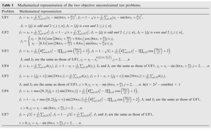
The performance of the TLBO was also evaluated for ten dif-ferent multi-objective unconstrained benchmark functions, UF1–UF10 (Zhang et al., 2008), against the other algorithms. The mathematical representations of these test functions are given in Tables 1 and 2. The unconstrained test functions, UF1–UF7, involve 2 objective functions, f1 and f2, that are to be minimized. The unconstrained test functions UF8– UF10 involve 3 objective functions, f1, f2and f3, that are to be minimized. Multiple objectives are combined into scalar objectives via a weight vector. All objective functions are nor-malized to have the same range.
3.2. Multi-objective constrained benchmark functions
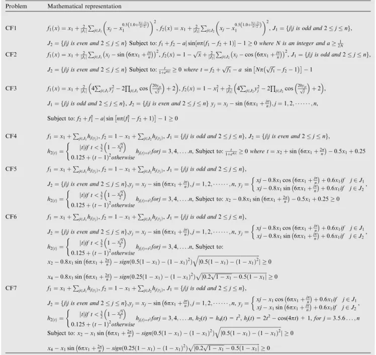
The performance of the TLBO algorithm was evaluated for se-ven different multi-objective constrained benchmark functions (CF1-CF7) (Zhang et al., 2008) against the other algorithms. The mathematical representations of these test functions are given inTable 3. The constrained test functions, CF1–CF7, in-volve 2 objective functions, f1and f2, that are to be minimized. Multiple objectives are combined into scalar objectives via a weight vector. All objective functions are normalized to have the same range. The TLBO algorithm was tested on the consid-ered benchmark functions provided for the CEC09 special ses-sion and competition on multi-objective optimization. The test suite is a collection of different characteristics of the Pareto front. IGD metric is used for each of the test functions to mea-sure the performance of the algorithm.
3.3. Performance metrics
Performance metric (IGD): LetP*be a set of uniformly dis-tributed points along the PF (in the objective space). Let A be an approximate set to the PF, the average distance from P*to A is defined using the following equation:
IGDðA;PÞ ¼ X #2p
ð#;AÞ
jPj ð14Þ
whered(#,A) is the minimum Euclidean distance between v and the points in A. If |P*| is sufficiently large to represent the Pareto front very well, both the diversity and convergence of the approximated set A could be measured usingIGD(A, P*). An optimization algorithm will attempt to minimize the value of theIGD(A,P*) measure.
3.4. Experimental settings
In these experiments, a population size of 50 and 125,000 func-tion evaluafunc-tions were considered for the SCH, ZDT1, ZDT2, ZDT3 and LZ functions. Moreover, a population size of 100 and 300,000 function evaluations was considered for
UF1–UF10 and CF1–CF7, and the algorithm was evaluated independently 30 times for each test problems. The TLBO was compared with the Archive-based Micro Genetic algo-rithm (AMGA) (Tiwari et al., 2009), Clustering Multi-objec-tive Evolutionary Algorithm (Clustering MOEA) (Wang et al., 2009), Differential Evolution with self-adaptation and Local Search algorithm (DECMOSA-SQP) (Zamuda et al., 2009), an improved version of the Dynamical Multi-Objective Evolutionary Algorithm (DMOEADD) (Liu et al., 2009), the Generalized Differential Evolution 3 (GDE3) (Kukkonen
and Lampinen, 2009), the LiuLi Algorithm (Liu and Li,
2009), a Multi-Objective Evolutionary Algorithm based on Decomposition (MOEAD) (Zhang et al., 2009), the Enhancing MOEA/D with Guided Mutation and Priority update (MOEADGM) (Chen et al., 2009), Multi-Objective Evolution-ary Programming (MOEP) (Qu and Suganthan, 2009), Multi-ple Trajectory Search (MTS) (Tseng and Chen, 2009), Local Search Based Evolutionary Multi-Objective Optimization Algorithm (NSGAIILS) (Sindhya et al., 2009), an improved algorithm based on An Efficient Multi-Objective evolutionary Figure 1 (a)–(e) The Pareto front obtained by the TLBO algorithm on unconstrained test functions SCH–ZDT1–ZDT2–ZDT3–LZ.
Algorithm (OMOEAII) (Gao et al., 2009), and Multi-Objec-tive Self-adapMulti-Objec-tive Differential Evolution Algorithm with objec-tive-wise Learning Strategies (OWMOSaDE) (Huang et al., 2009) methods on unconstrained test problems and con-strained test problems. A brief description of these algorithms is presented in this section and the detailed mathematical for-mulations of these algorithms are available in the above refer-ences. Generalized Differential Evolution 3 (GDE3) is an extension of differential evolution (DE) for global optimiza-tion with an arbitrary number of objectives and constraints.
For a problem with a single objective and without constraints, GDE3 falls back to the original DE. GDE3 improves earlier GDE versions for multi-objective problems by yielding a bet-ter-distributed solution. The Archive-based Micro Genetic algorithm (AMGA) is an evolutionary optimization algorithm that relies on genetic variation operators to create new solu-tions. The generation scheme deployed in the algorithm can be classified as generational, only solutions that are created prior to a particular iteration take part in the selection process during the said iteration (generation). However, the algorithm Table 1 Mathematical representation of the two objective unconstrained test problems.
Problem Mathematical representation UF1 f1¼x1þjJ2 1j P j2J1½xjsinð6px1þjpnÞ 2 ,f2¼1 p xþ 2 jJ1j P j2J2½xjsinð6px1þjpnÞ 2 , J1¼fjjj is odd and2jng;J2¼fjjj is even and2jng
UF2 f1¼x1þjJ21j P j2J1y2j,f2¼1 p xþ 2 jJ1j P
j2J2y2j,J1¼fjjj is odd and2jng,J2¼fjjj is even and2jng, yj¼ xj 0:3x2 1cos 24p x1þ4njpþ0:6x1cos 6p x1þjnpj2j1 xj 0:3x12cos 24px1þ4njp þ0:6x1 sinð6px1þjnpÞj2j2 ( UF3 f1¼x1þjJ21j 4 P j2J1y2j 2 Q j2J1cos 20jjp ffi j p þ2 ,f2¼1pffiffiffiffiffix2þjJ21j 4 P j2J1y2j 2 Q j2J2cos 20jjp ffi j p þ2
J1and J2are the same as those of UF1,yj¼xjx 0:5 1:0þ3ðj2Þ n2 ð Þ 1 ;j¼2;. . .;n UF4 f1¼x1þjJ21j P j2J1hðyjÞ,f2¼1x2þjJ22j P
j2J2hðyjÞ, J1and J2are the same as those of UF1,yj¼xjsin 6px1þjnp
;j¼2;. . .;n UF5 f1¼x1þ21Nþ 2jsinð2Npx1Þj þjJ21j P j2J1hðyjÞ,f2¼1x1þ21Nþ 2jsinð2Npx1Þj þjJ22j P j2J2hðyjÞ, J1and J2are the same as those of UF1,e>0;yj¼xjsin 6px1þjpn
;j¼2;. . .;n:h(t) = 2t2cos(4pt) + 1 UF6 f1¼x1þmax 0;2 21Nþ 2 sinð2Npx1Þ þ 2 jj1j 4 P j2J1y2j2 Q j2J1cos 20jjffip j p þ2 , f1¼1x1þmax 0;221Nþ 2 sinð2Npx1Þ 2 jj2j 4 P j2J2y2j2 Q j2J2cos 20jjffip j p þ2
, J1and J2are the same as those of UF1,
e>0;yj¼xjsin 6px1þjnp ;j¼2;. . .;n: UF7 f1¼p5ffiffiffiffiffix1þjj21j P j2J1y2j,f2¼1p5ffiffiffiffiffix1þjj21j P
j2J2y2j,J1andJ2are the same as those of UF1,
e>0;yj¼xjsin 6px1þjnp
;j¼2;. . .;n:
Table 2 Mathematical representation of the three objective unconstrained test problems.
Problem Mathematical representation UF8 f1¼cosð0:5x1pÞcosð0:5x2pÞ þjJ21j
P j2J1 xj2x2sin 2px1þ jp n 2 ,f2¼cosð0:5x1pÞsinð0:5x2pÞ þjJ22j P j2J1 xj2x2sin 2px1þ jp n 2 , f3¼sinð0:5x1pÞ þjJ21j P j2J1 xj2x2sin 2px1þ jp n 2 ,J1¼ fjj jn; and j1is a multiplication of3g, J2¼ fjj jn; and j2is a multiplication of3g,J3¼ fjj jn;and j is a multiplication of3g UF9 f1¼0:5 max 0;ð1þeÞ 14 2ð x11Þ2 n o þ2x1 h i x2þjJ21j P j2J1 xj2x2sin 2px1þjnp 2 , f2¼0:5 max 0;ð1þeÞ 14 2ð x11Þ2 n o þ2x1 h i x2þjJ22j P j2J2 xj2x2sin 2px1þjnp 2 , f3¼1x2þjJ23j P j2J3 xj2x2sin 2px1þ jp n 2 ,J1¼ fjj jn;and j1is a multiplication of3g, J2¼ fjj jn;and j2is a multiplication of3g,J3¼ fjj jn;and j is a multiplication of3gande¼0:1 UF10 f1¼cosð0:5x1pÞcosð0:5x2pÞ þjJ21j
P
j2J1½4y2jcosð8py1Þ þ1,f2¼cosð0:5x1pÞsinð0:5x2pÞ þjJ21j P
j2J1½4y2j cosð8py1Þ þ1, f3¼sinð0:5x1pÞ þjJ21j
P
j2J1½4yj2cosð8py1Þ þ1,J1¼ fjj jn; and j1is a multiplication of3g, J2¼ fjj jn; and j2is a multiplication of3g,J3¼ fjj jn;and jis a multiplication of3g
generates a small number of new solutions at each iteration. Therefore, it can also be classified as an almost steady-state ge-netic algorithm. The algorithm operates with a small popula-tion size and maintains an external archive of good obtained solutions. A small number of solutions are created at each iter-ation using the genetic variiter-ation operators. The newly created solutions are then used to update the archive. The AMGA operates with a very small population size and uses an external archive to maintain its search history. The use of a large ar-chive is recommended to obtain a large number of non-domi-nated solutions. The size of the archive determines the computational complexity of the algorithm. However, for computationally expensive optimization problems, the actual time taken by the algorithm is negligible compared to the time
taken by the analysis routines. The parent population is created from the archive, and binary tournament selection is performed on the parent population to create the mating pop-ulation. The design of the algorithm is independent of the Table 3 Mathematical representation of the constrained test problems (CF1–CF7).
Problem Mathematical representation
CF1 f1ðxÞ ¼x1þjJ21j P j2J1 xjx 0:5 1ð:0þ3nðj22ÞÞ 1 2 ,f2ðxÞ ¼x1þjJ22j P j2J2 xjx 0:5 1ð:0þ3nðj22ÞÞ 1 2 ,J1¼fjjj is odd and2jng, J2¼fjjj is even and2jngSubject to:f1þf2ajsin½npðf1f2þ1Þ 10where N is an integer and a21N CF2 f1ðxÞ ¼x1þjJ21j P j2J1 xjsin 6px1þ jp n 2 ,f2ðxÞ ¼1 ffiffiffix p þ 2 jJ2j P j2J2 xjcos 6px1þ jp n 2 ,J1¼fjjj is odd and2jng, J2¼fjjj is even and2jngSubject to:1þte4jtj0where t¼f2þ ffiffiffiffif1
p a sin Np ffiffiffiffif1 p f21 1 CF3 f1ðxÞ ¼x1þjJ21j 4 P j2J1y 2 j 2 Q j2J1cos 20yffijp j p þ2 ,f2ðxÞ ¼1x21þjJ22j 4 P j2J2y 2 j2 Q j2J2cos 20yffijp j p þ2 , J1¼fjjj is odd and2jng,J2¼fjjj is even and2jngyj¼xjsin 6px1þjnp
;j¼1;2; ;n, Subject to:f2þf21ajsin npðf21f2þ1Þ10
CF4 f1¼x1þPj2J1hjðyjÞ,f2¼1x1þ P
j2J2hjðyjÞ,J1¼fjjj is odd and2jng,J2¼fjjj is even and2jng,
h2ðtÞ¼ jtjif t<3 2 1 ffiffi 2 p 2 0:125þ ðt1Þ2otherwise (
hjðtÞ¼t2forj¼3;4;. . .:n, Subject to: t
1þe4jtj0where t¼x2þsin 6px1þ2np 0:5x1þ0:25 CF5 f1¼x1þPj2J1hjðyjÞ,f2¼1x1þ P j2J2hjðyjÞ,J1¼fjjj is odd and2jng,
J2¼fjjj is even and2jng,yj¼xjsin 6px1þjnp
;j¼1;2; ;n,yj¼ xj0:8x1cos 6p x1þjnpþ0:6x1if j2J1 xj0:8x1sin 6p x1þjnpþ0:6x1if j2J2 , h2ðtÞ¼ jtjif t<3 2 1 ffiffi 2 p 2 0:125þ ðt1Þ2otherwise (
hjðtÞ¼t2forj¼3;4;. . .:n, Subject to:x20:8x1sin 6px1þ2np
0:5x1þ0:250 CF6 f1¼x1þPj2J1hjðyjÞ,f2¼1x1þ
P
j2J2hjðyjÞ,J1¼fjjj is odd and2jng,
J2¼fjjj is even and2jng,yj¼xjsin 6p x1þjnp;j¼1;2; ;n,yj¼
xj0:8x1cos 6px1þjnp þ0:6x1if j2J1 xj0:8x1sin 6px1þjnp þ0:6x1if j2J2 , h2ðtÞ¼ j tjif t<3 2 1 ffiffi 2 p 2 0:125þ ðt1Þ2otherwise (
hjðtÞ¼t2forj¼3;4;. . .:n, Subject to:
x20:8x1sin 6px1þ2np signð0:5ð1x1Þ ð1x1Þ2Þ ffiffiffiffiffiffiffiffiffiffiffiffiffiffiffiffiffiffiffiffiffiffiffiffiffiffiffiffiffiffiffiffiffiffiffiffiffiffiffiffiffiffiffiffiffiffiffiffiffi j0:5ð1x1Þ ð1x1Þ2 q j 0 x40:8x1sin 6px1þ2np signð0:25ð1x1Þ ð1x1Þ2Þ ffiffiffiffiffiffiffiffiffiffiffiffiffiffiffiffiffiffiffiffiffiffiffiffiffiffiffiffiffiffiffiffiffiffiffiffiffiffiffiffiffiffiffiffiffiffiffiffiffiffiffiffiffi j0:2 ffiffiffiffiffiffiffiffiffiffiffiffiffi1x1 p 0:5ð1x1j p 0 CF7 f1¼x1þPj2J1hjðyjÞ,f2¼1x1þ P j2J2hjðyjÞ,J1¼fjjj is odd and2jng,
J2¼fjjj is even and2jng,yj¼xjsin 6p x1þjnp;j¼1;2; ;n,yj¼
xjx1cos 6px1þjnp þ0:6x1if j2J1 xjx1sin 6px1þjnp þ0:6x1if j2J2 , h2ðtÞ¼ j tjif t<3 2 1 ffiffi 2 p 2 0:125þ ðt1Þ2otherwise (
hjðtÞ¼t2forj¼3;4;. . .:n,h2(t) =h4(t) =t2,hj(t) = 2t2cos(4pt) + 1,for j¼3:5:6. . .;n
Subject to:x2x1sin 6p x1þ2npsignð0:5ð1x1Þ ð1x1Þ2Þ
ffiffiffiffiffiffiffiffiffiffiffiffiffiffiffiffiffiffiffiffiffiffiffiffiffiffiffiffiffiffiffiffiffiffiffiffiffiffiffiffiffiffiffiffiffiffiffiffiffi j0:5ð1x1Þ ð1x1Þ2 q j 0 x4x1sin 6px1þ2np signð0:25ð1x1Þ ð1x1Þ2Þ ffiffiffiffiffiffiffiffiffiffiffiffiffiffiffiffiffiffiffiffiffiffiffiffiffiffiffiffiffiffiffiffiffiffiffiffiffiffiffiffiffiffiffiffiffiffiffiffiffiffiffiffiffi j0:2 ffiffiffiffiffiffiffiffiffiffiffiffiffi1x1 p 0:5ð1x1j p 0
Table 4 Summary of results.
Functions Errors (1000 iterations) Errors (2500 iterations)
SCH 4.3E-09 5.6E-26
ZDT1 1.1E-6 2.6E-23
ZDT2 7.1E-6 3.2E-19
ZDT3 2.1E-5 4.1E-17
encoding of the variables. Thus the algorithm can operate with almost any type of encoding (so long as suitable genetic varia-tion operators are provided to the algorithm). The algorithm uses the concept of Pareto ranking borrowed from NSGA-II and is based on a two-tier fitness mechanism.
The LiuLi Algorithm is a multi-objective optimization algo-rithm based on sub-regional search, which forces individuals in the same region operate with each other via an evolutionary operator, and the information between the individuals of different regions is exchanged via their offspring and again re-divided into regions. The multi-objective Evolutionary Algorithm based on Decomposition (MOEAD) is a objective evolutionary algorithm that decomposes a multi-objective optimization problem into a number of scalar optimization sub-problems and optimizes them simulta-neously. Each sub-problem is optimized by only using infor-mation from its several neighboring sub problems, which reduces the computational complexity of MOEAD at each generation compared to the non-dominated sorting genetic algorithm II (NSGA-II). Multiple Trajectory Search (MTS) uses multiple agents to concurrently search the solution space. Each agent performs an iterated local search using one of the three candidate local search methods. By choosing a local search method that best fits the landscape of a solution’s neigh-borhood, an agent may find its way to a local optimum or the global optimum. Multi-objective self-adaptive Differential Evolution Algorithm with objective-wise Learning Strategies
(OWMOSaDE) learns suitable crossover parameter values and mutation strategies for each objective separately in a mul-ti-objective optimization problem. An improved algorithm based on an Efficient Multi-objective evolutionary algorithm (OMOEAII) uses a new linear breeding operator with lower-dimensional crossover and copy operation. With the lower-dimensional crossover, the complexity of the search is decreased, which allows the algorithm to converge faster. The orthogonal crossover increases the probability of produc-ing potentially superior solutions, which helps the algorithm obtain better results.
4. Experimental results and discussion
In this section, TLBO was applied on several benchmark prob-lems to evaluate its performance, including the set of bench-mark functions provided for the CEC09 special session and competition on multi-objective optimization. All tests were evaluated on an Intel core i3 2.53 GHz processor. The algo-rithm was coded using the Matlab programming language. This section contains the computational results obtained by the TLBO algorithm compared to other multi-objective meth-ods over a set of test problems. The performance measures are summarized in Table 5in terms of generalized distance Dg. This table clearly shows that TLBO yielded best results for all the multi-objective test functions, SCH, ZDT1, ZDT2, ZDT3 and LZ, and obtained the first rank of eight algorithms.
Table 5 Comparison of Dg forn= 50 andt= 500 iterations.
Methods ZDT1 ZDT2 ZDT3 SCH LZ
VEGA (Schaffer, 1985) 3.79E-02 2.37E-03 3.29E-01 6.98E-02 1.47E-03
NSGA-II (Deb et al., 2002) 3.33E-02 7.24E-02 1.14E-01 5.73E-03 2.77E-02
MODE (Babu and Gujarathi, 2007) 5.80E-03 5.50E-03 2.15E-02 9.32E-04 3.19E-03 DEMO (Robic and Filipic, 2005) 1.08E-03 7.55E-04 1.18E-03 1.79E-04 1.40E-03 Bees (Pham and Ghanbarzadeh, 2007) 2.40E-02 1.69E-02 1.91E-01 1.25E-02 1.88E-02
SPEA (Deb et al., 2002) 1.78E-03 1.34E-03 4.75E-02 5.17E-03 1.92E-03
MOFA (Yang, 2012) 1.90E-04 1.52E-04 1.97E-04 4.55E-06 8.70E-04
TLBO 1.12E-07 1.70E-06 1.61E-06 9.99E-07 1.27E-06
The bold values indicate the best performance.
Table 6 The mean value of IGD used for each test instance UF1–UF7.
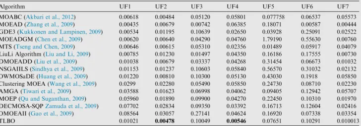
Algorithm UF1 UF2 UF3 UF4 UF5 UF6 UF7
MOABC (Akbari et al., 2012) 0.00618 0.00484 0.05120 0.05801 0.077758 0.06537 0.05573 MOEAD (Zhang et al., 2009) 0.00435 0.00679 0.00742 0.06385 0.18071 0.00587 0.00444 GDE3 (Kukkonen and Lampinen, 2009) 0.00534 0.01195 0.10639 0.02650 0.03928 0.25091 0.02522 MOEADGM (Chen et al., 2009) 0.00620 0.00640 0.04290 0.04760 1.79190 0.55630 0.00760 MTS (Tseng and Chen, 2009) 0.00646 0.00615 0.05310 0.02356 0.01489 0.05917 0.04079 LiuLi Algorithm (Liu and Li, 2009) 0.00785 0.01230 0.01497 0.04350 0.16186 0.17555 0.00730 DMOEADD (Liu et al., 2009) 0.01038 0.00679 0.03337 0.04268 0.31454 0.06673 0.01032 NSGAIILS (Sindhya et al., 2009) 0.01153 0.01237 0.10603 0.05840 0.56570 0.31032 0.02132 OWMOSaDE (Huang et al., 2009) 0.01220 0.00810 0.10300 0.05130 0.43030 0.1918 0.05850 Clustering MOEA (Wang et al., 2009) 0.0299 0.02280 0.05490 0.05850 0.24730 0.08710 0.02230 AMGA (Tiwari et al., 2009) 0.03588 0.01623 0.06998 0.04062 0.09405 0.12942 0.05707 MOEP (Qu and Suganthan, 2009) 0.05960 0.01890 0.09900 0.04270 0.22450 0.10310 0.01970 DECMOSA-SQPZamuda et al., 2009) 0.07702 0.02834 0.09350 0.03392 0.16713 0.12604 0.02416 OMOEAII (Gao et al., 2009) 0.08564 0.03057 0.27141 0.04624 0.16920 0.07338 0.03354
TLBO 0.01021 0.00478 0.10049 0.00546 0.07651 0.10291 0.010013
The results of all functions are summarized inTable 4, and the estimated Pareto fronts and true fronts of SCH, ZDT1, ZDT2, ZDT3 and LZ are shown inFig. 1.Fig. 1shows that the TLBO successfully converges to the optimal Pareto front, and its approximation well distributed.
The mathematical representations of the UF1–UF10 and the CF1–CF7 test problems are given inTables 1–3. The com-parisons of the results of seven multi-objective unconstrained functions with other algorithms are given inTable 6, and the estimated Pareto fronts and true fronts of the unconstrained functions are shown inFig. 2.
For the UF1 test problem, the TLBO algorithm obtained the seventh rank of 15 algorithms. In addition to the quantita-tive comparison of the investigated algorithm, the graphical representations of the Pareto fronts produced by the TLBO algorithm are given in Fig. 2. This figure shows the quality of the Pareto fronts produced by the TLBO algorithm.
Fig. 2(a) shows that the results produced not only converged well, but were also appropriately distributed over the Pareto front in the objective space. The TLBO algorithm outper-formed other algorithms when optimizing the UF2 test prob-lem. The TLBO obtained the first rank for the UF2 test Figure 2 (a)–(j) The Pareto front obtained by the TLBO algorithm on unconstrained test functions UF1–UF10.
problem.Fig. 2(b) shows that the produced Pareto front was uniformly distributed. For the UF3 test problem, the TLBO
obtained the eleventh rank of 15 algorithms. The best conver-gence was obtained by the MOEAD algorithm. However, the Fig. 2(continued)
Table 7 The mean value of IGD used for each test instance UF8–UF10.
Algorithm UF8 UF9 UF10
MOABC (Akbari et al., 2012) 0.06726 0.06150 0.19499
MOEAD (Zhang et al., 2009) 0.05840 0.07896 0.047415
GDE3 (Kukkonen and Lampinen, 2009) 0.24855 0.08248 0.43326
MOEADGM (Chen et al., 2009) 0.24460 0.18780 0.5646
MTS (Tseng and Chen, 2009) 0.11251 0.11442 0.15306
LiuLi Algorithm (Liu and Li, 2009) 0.08235 0.09391 0.44691
DMOEADD (Liu et al., 2009) 0.06841 0.04896 0.32211
NSGAIILS (Sindhya et al., 2009) 0.08630 0.07190 0.84468
OWMOSaDE (Huang et al., 2009) 0.09450 0.09830 0.74300
Clustering MOEA (Wang et al., 2009) 0.23830 0.29340 0.41110
AMGA (Tiwari et al., 2009) 0.17125 0.18861 0.32418
MOEP (Qu and Suganthan, 2009) 0.42300 0.34200 0.36210
DECMOSA-SQPZamuda et al., 2009) 0.21583 0.14111 0.36985
OMOEAII (Gao et al., 2009) 0.19200 0.23179 0.62754
TLBO 0.004933 0.011639 0.03823
TLBO algorithm can produce uniformly distributed Pareto fronts, as shown inFig. 2(c). The TLBO algorithm obtained the best result for the UF4 test problem and obtained first rank of 15 algorithms. Fig. 2(d) shows the quality of the Pareto
front for the UF4 test problem. The UF5 seemingly constitutes a difficult problem to solve. The TLBO algorithm obtained the third rank of 15 algorithms.Fig. 2(e) shows that the TLBO algorithm produces an archive in which its members are Table 8 The mean value of IGD used for each test instance CF1–CF7.
Algorithm CF1 CF2 CF3 CF4 CF5 CF6 CF7
MOABC (Akbari et al., 2012) 0.00992 0.01027 0.08621 0.00452 0.06781 0.00483 0.01692 GDE3 (Kukkonen and Lampinen, 2009) 0.02940 0.01597 0.12750 0.00799 0.06799 0.06199 0.04169 MOEADGM (Chen et al., 2009) 0.01080 0.00800 0.51340 0.07070 0.54460 0.20710 0.53560 MTS (Tseng and Chen, 2009) 0.01918 0.02677 0.10446 0.01109 0.02077 0.01616 0.02469 LiuLi Algorithm (Liu and Li, 2009) 0.00085 0.00420 0.18290 0.01423 0.10973 0.01394 0.10446 DMOEADD (Liu et al., 2009) 0.01131 0.00210 0.05630 0.00699 0.01577 0.01502 0.01905 NSGAIILS (Sindhya et al., 2009) 0.00692 0.01183 0.23994 0.01576 0.18420 0.02013 023345 DECMOSA-SQP (Zamunda et al., 2009) 0.10773 0.09460 1000000 0.15265 0.41275 0.14782 0.26049
TLBO 0.0088 0.000140 0.002415 0.001305 0.01236 0.001359 0.005270
The bold values indicate the best performance.
uniformly distributed over the Pareto fronts. For the UF6 test problems, the TLBO algorithm obtained the seventh rank of 15 algorithms. The UF6 contains a discontinuous Pareto front. Hence, an optimization algorithm needs to give preference to the Pareto front and move the archive members to the parts of solution space that contain the members of the Pareto fronts. The results show that most of the algorithms have dif-ficulty in optimizing this type of test problems.Fig. 2(f) shows that the TLBO algorithm produces competitive results for this
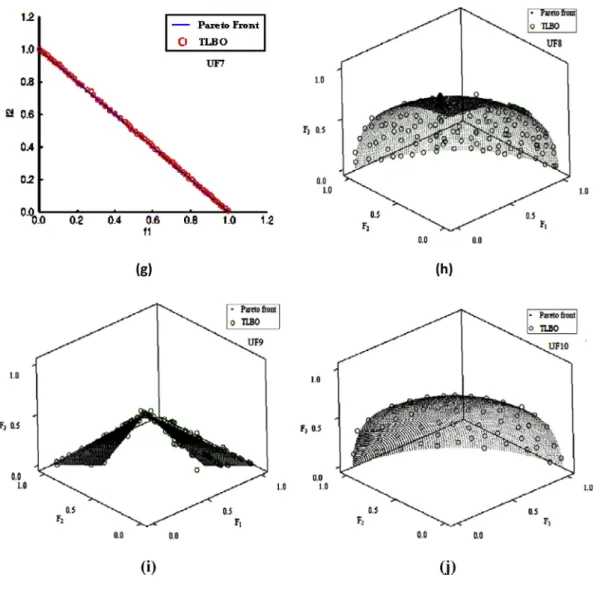
test problem. For the UF7 test problem, the TLBO algorithm obtained the fourth rank of 15 algorithms. Although the MOABC converged well over the optimal Pareto front, the top-left corner of the Pareto front was not successfully covered by the MOABC algorithm, which was covered by the TLBO algorithm. Hence, the TLBO obtained competitive results for the UF7 test problem (Fig. 2(g)).
Usually, the complexity of multi-objective problems posi-tively correlates with the number of objectives to be optimized. Fig. 3(continued)
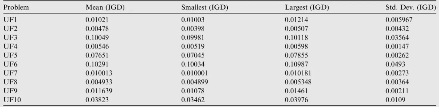
Table 9 The IGD statistics over UF1–UF10.
Problem Mean (IGD) Smallest (IGD) Largest (IGD) Std. Dev. (IGD)
UF1 0.01021 0.01003 0.01214 0.005967 UF2 0.00478 0.00398 0.00507 0.00432 UF3 0.10049 0.09981 0.10118 0.03564 UF4 0.00546 0.00519 0.00598 0.00147 UF5 0.07651 0.07045 0.07855 0.00262 UF6 0.10291 0.10034 0.10987 0.0493 UF7 0.010013 0.010001 0.010181 0.00273 UF8 0.004933 0.004899 0.005348 0.00364 UF9 0.011639 0.01078 0.01461 0.00211 UF10 0.03823 0.03462 0.03976 0.0109
The results of three objective unconstrained functions are com-pared with other algorithms in Table 7. For the first three objectives of the UF8 test problem, the TLBO algorithm ob-tained the best result and first rank of 15 algorithms. The qual-ity of the approximated Pareto front is shown inFig. 2(h). The results indicate that the TLBO produced a set of solution points that are appropriately distributed in the 3-dimensional objective space. Again, the TLBO obtained the first rank for the UF9 test problem. The quality of the approximated Pareto front is demonstrated inFig. 2(i). The results show that the TLBO produces a set of non-dominated points that cover a large part of the objective space. For the UF10 test problem, the TLBO also obtained the first rank and the best result of 15 algorithms.Fig. 2(j) demonstrates the quality of the approx-imated Pareto front obtained by the TLBO algorithm. The re-sults show that the approximated Pareto front covers a large part of the objective space. However, compared to the approx-imated Pareto fronts of the UF8 and UF9, the TLBO algo-rithm produces a small number of points in the objective space.
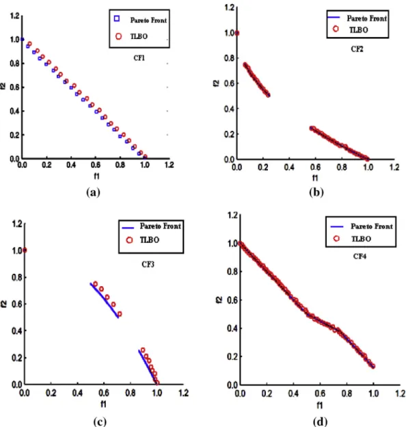
Table 8compares the results of seven multi-objective con-strained functions with other algorithms, and the estimated Pareto fronts and true fronts of constrained functions are shown inFig. 3. The TLBO algorithm obtained the third rank for the CF1 test problem of 9 algorithms. The LiuLi Algorithm performed best for this test problem. The quality of the approximated Pareto front is shown inFig. 3(a) for the CF1 test problem. The CF1 features a discontinuous Pareto front. The TLBO algorithm successfully solved the CF2 test problem. The TLBO obtained the first rank for the CF2 test problem. The quality of the approximated Pareto front in Fig. 3(b) shows that the TLBO successfully converges to the optimal Pareto front. However, discontinuities persisted in the produced solutions of the TLBO algorithm. The TLBO algo-rithm obtained the first rank of 9 algoalgo-rithms for the CF3 test problem. Most of the algorithms showed difficulty in solving the CF3 test problem. The TLBO produced a small number of solutions for this test problem. The quality of the approxi-mated Pareto front is shown inFig. 3(c) for the CF3 test prob-lem. The TLBO algorithm successfully solved the CF4 test problem and obtained the first rank.Fig. 3(d) shows that the TLBO algorithm produced a set of solutions that were uni-formly distributed over the Pareto front. For the CF5 test problem, TLBO obtained the first rank of 9 algorithms.
Fig. 3(e) shows that the TLBO successfully converged to the optimal Pareto front. However, most of the produced solu-tions gravitated to the left corner of the Pareto front, and the TLBO algorithm did not obtained a uniform distribution of the solutions, but distribution of the solution was better than that of the MOABC algorithm. The TLBO successfully solved the CF6 test problem and obtained the first rank.
Fig. 3(f) shows that the TLBO successfully converged to the optimal Pareto front, and its approximation was well distrib-uted. The TLBO algorithm obtained the first rank for the CF7 test problem of the 9 algorithms. Even though the MOA-BC can successfully converge to the optimal solution, the produced solutions lacked a uniform distribution. However, the TLBO can successfully converge to the optimal solutions and produced uniformly distributed solutions as shown in
Fig. 3(g). Hence, the TLBO algorithm surpasses other
algo-rithms in solving CF3, CF4, CF5, CF6 and CF7 test problems.
Rao and Patel (2012) calculated the computational
com-plexity of the TLBO algorithm considering the G-functions of CEC 2006 and reported a value of 0.2615, which was con-siderably better than those calculated by the other algorithms, except for the Particle Evolutionary Swarm Optimization Plus (PESO+) algorithm (i.e., 0.2527 for PESO+, 0.4685 for Dif-ferential Evolution with Gradient-Based Mutation and Feasi-ble Elites, 0.6958 for Self-adaptive Differential Evolution Algorithm, 1.0581 for Dynamic Multi-Swarm Particle Swarm optimizer, 1.57654 for Differential Evolution, 1.981464 for Modified Differential Evolution, 2.0245 for Generalized Dif-ferential Evolution, 2.386 for Population-Based Parent Centric Procedure, 5.5329 for PSO and 11.37 for Approximate Evolu-tion Strategy using Stochastic Ranking). For more details on the G-functions of CEC 2006 and the results of various optimi-zation algorithms, the readers may refer toLiang et al. (2006). Thus, the TLBO algorithm is comparatively less computation-ally complex. However, the computational complexity of the TLBO algorithm for the functions considered in this paper was not calculated, as this calculation is beyond the scope of this paper. The value of 0.2615 presented by Rao and Patel (2012)for the G-functions of CEC 2006 hints at comparatively lessened computational complexity of the TLBO algorithm. Interestingly, the results obtained by the TLBO algorithm are comparable to those given in Rao and Patel (2014)and even better in some cases with less effort. The overall perfor-mance shows that the TLBO algorithm can be used as an effec-tive tool to optimize problems with multiple objeceffec-tives.
5. Conclusion
Multi-objective optimization is a very important research area in engineering studies, because real-world design problems require the optimization of a group of objectives. Multiple, of-ten conflicting, objectives arise naturally in most real-world optimization scenarios. Adding more than one objective to an optimization problem adds complexity. In this paper, the performance of the TLBO algorithm was verified with well-known other optimization methods, such as AMGA,
Table 10 The IGD statistics over CF1–CF7.
Problem Mean (IGD) Smallest (IGD) Largest (IGD) Std. Dev. (IGD)
CF1 0.0088 0.0049 0.0098 0.00061 CF2 0.000140 0.000129 0.000187 0.00048 CF3 0.002415 0.002256 0.002578 0.00713 CF4 0.001305 0.001277 0.001401 0.00083 CF5 0.01236 0.01210 0.01293 0.01981 CF6 0.001359 0.001314 0.001388 0.00021 CF7 0.005270 0.005205 0.005314 0.00452
Clustering MOEA, DECMOSA-SQP, DMOEADD, GDE3, LiuLi Algorithm, MOEAD, MOEADGM, etc. by experiment-ing with different multi-objective unconstrained and con-strained benchmark functions. The experimental results show that the TLBO performs competitively with other optimization methods reported in the literature. Therefore, the TLBO algo-rithm is effective and robust and has a great potential for solv-ing multi-objective problems. The TLBO will be tested with more complex functions in the near future (seeTables 9 and 10).
References
Ahrari, A., Atai, A.A., 2010. Grenade explosion method - A novel tool for optimization of multimodal functions. Appl. Soft Comput. 10 (4), 1132–1140.
Akbari, R., Hedayatzadeh, R., Ziarati, K., Hassanizadeh, B., 2012. A muti-objective artificial bee colony algorithm. Swarm Evol. Com-put. 2, 39–52.
Akay, B., Karaboga, D., 2012. Artificial bee colony algorithm for large-scale problems and engineering design optimization. J. Intell. Manuf. 23, 1001–1014.
Awadallah, M.A., Khader, A.T., Al-Betar, M.A., Bolaji, A.L., 2013. Global best Harmony Search with a new pitch adjustment designed for Nurse Rostering. J. King Saud University – Comput. Inf. Sci. 25, 145–162.
Babu, B.V., Gujarathi, A.M., 2007. Multi-objective differential evo-lution (MODE) for optimization of supply chain planning and management. In: IEEE congress on evolutionary computation, (CEC 2007), pp. 2732–2739.
Blum, C., 2005. Ant colony optimization: Introduction and recent trends. Phys. Life Rev., 353–373.
Chen, C.M., Chen, Y., Zhang, Q., 2009. Enhancing MOEA/D with guided mutation and priority update for multi-objective optimiza-tion. In: Proceeding of Congress on Evolutionary Computation, CEC’09, pp. 209–216.
Clerc, M., 2006. Particle Swarm Optimization. ISTE Publishing Company.
Deb, K., Pratap, A., Agarwal, S., Mayarivam, T., 2002. A fast and elitist multiobjective algorithm: NSGA-II. IEEE Trans. Evol. Comput. 6, 182–197.
Dorigo, M., Stutzle, T., 2004. Ant Colony Optimization. MIT Press. Fahmy, A.A., 2012. Using the Bees Algorithm to select the optimal
speed parameters for wind turbine generators. J. King Saud University Comput. Inf. Sci. 24, 17–26.
Gao, S., Zeng, S., Xiao, B., Zhang, L., Shi, Y., Yang, X., Yu, D., Yan, Z., 2009. An orthogonal multi-objective evolutionary algorithm with lower-dimensional crossover. In: Proceeding of Congress on Evolutionary Computation, CEC’09, pp. 1959–1964.
Goldberg, D., 1989. Genetic Algorithms in Search, Optimization, and Machine Learning. Addidon-Wesley, New York.
Goswami, B., Mandal, D., 2013. A genetic algorithm for the level control of nulls and side lobes in linear antenna arrays. J. King Saud Univ. Comput. Inf. Sci. 25, 117–126.
Hartikainen, M., Miettinen, K., Wiecek, M., 2012. PAINT: Pareto front interpolation for nonlinear multiobjective optimization. Comput. Optim. Appl. 52, 845–867.
He, Q., Wang, L., 2007. An effective co-evolutionary particle swarm optimization for constrained engineering design problems. Eng. Appl. Artif. Intell. 20, 89–99.
Huang, V.L., Zhao, S.Z., Mallipeddi, R., Suganthan, P.N., 2009. Multi-objective optimization using self-adaptive differential evolu-tion algorithm. In: Proceeding of Congress on Evoluevolu-tionary Computation, CEC’09, pp. 190–194.
Karaboga, D., Basturk, B., 2008. On the performance of artificial bee colony (ABC) algorithm. Appl. Soft Comput. 8, 687– 697.
Karaboga, D., 2005. An idea based on honey bee swarm for numerical optimization. Technical report-TR06. Erciyes University, Engi-neering Faculty, Computer EngiEngi-neering Department.
Kennedy, V., Eberhart, R., 1995. Particle swarm optimization. In: Proceedings of the IEEE International Conference on Neural Networks, pp.1942–1948.
Kukkonen, S., Lampinen, J., 2009. Performance assessment of generalized differential evolution with a given set of constrained multi-objective test problems. In: Proceeding of Congress on Evolutionary Computation, CEC’09, pp. 1943–1950.
Lee, K.S., Geem, Z.W., 2004. A new meta-heuristic algorithm for continuous engineering optimization: harmony search theory and practice. Comput. Methods Appl. Mech. Eng. 194, 3902–3933. Liang, J.J., Runarsson, T.P., Mezura-Montes, E., Clerc, M.,
Sugan-than, P.N., Coello, C.A.C, Deb, K. 2006. Problem definitions and evaluation criteria for the CEC special session on constrained real parameter optimization. Technical Report, Nanyang Technological University, Singapore.
Liu, H., Li, X., 2009. The multi-objective evolutionary algorithm based on determined weight and sub-regional search. In: Proceeding of Congress on Evolutionary Computation, CEC’09, pp. 1928–1934. Liu, M., Zou, X., Chen, Y., Wu, Z., 2009. Performance assessment of
DMOEA-DD with CEC 2009 moea competition test instances. In: Proceeding of Congress on Evolutionary Computation, CEC’09, pp. 2913–2918.
Liu, H., Cai, Z., Wang, Y., 2010. Hybridizing particle swarm optimization with differential evolution for constrained numerical and engineering optimization. Appl. Soft Comput. 10, 629–640. Madavan, N.K., 2002. Multiobjective optimization using a pareto
differential evolution approach. In: Congress on Evolutionary Computation 2, pp. 1145–1150.
Mandal, S., Ghoshal, S.P., Kar, R., Mandal, D., 2012. Design of optimal linear phase FIR high pass filter using craziness based particle swarm optimization technique. J. King Saud Univ. Comput. Inf. Sci. 24, 83–92.
Parsopoulos, K.E., Vrahatis, M.N., 2005. In: Wang, L. (Ed.), . In: Unified Particle Swarm Optimization for Solving Constrained Engineering Optimization Problems, vol. 3612. LNCS (ICNC), pp. 581–582.
Pham, D.T., Ghanbarzadeh, A., 2007. Multi-objective optimization using the bees algorithm. In: 3rd international virtual conference on intelligent production machines and systems (IPROMS 2007) Whittles, Dunnbeath, Scotland.
Qu, B.Y., Suganthan, P.N., 2009. Multi-objective evolutionary programming without non-domination sorting is up to twenty times faster. In: Proceeding of Congress on Evolutionary Compu-tation, CEC’09, pp. 2934–2939.
Rao, R.V., Savsani, V.J., Vakharia, D.P., 2011. Teaching–learning-based optimization: a novel method for constrained mechanical design optimization problems. Computer-Aided Des. 43, 303–315. Rao, R.V., Savsani, V.J., Balic, J., 2012a. Teaching–learning-based optimization algorithm for unconstrained and constrained real parameter optimization problems. Eng. Optim. 44 (12), 1447–1462. Rao, R.V., Savsani, V.J., Vakharia, D.P., 2012b. Teaching–learning-based optimization: a novel optimization method for continuous non-linear large scale problems. Inf. Sci. 183 (1), 1–15.
Rao, R.V., Savsani, V.J., 2012. Mechanical Design Optimization using Advanced Optimization Techniques. Springer-Verlag, London. Rao, R.V., Patel, V., 2012. An elitist teaching–learning-based
optimi-zation algorithm for solving complex constrained optimioptimi-zation problems. Int. J. Indus. Eng. Comput. 3 (4), 535–560.
Rao, R.V., Patel, V., 2014. A multi-objective improved teaching– learning-based optimization algorithm for unconstrained and constrained optimization problems. Int. J. Indus. Eng. Computat. 5.http://dx.doi.org/10.5267/j.ijiec.2013.09.007.
Robic, T., Filipic, B., 2005. DEMO: differential evolution for multiobjective optimization. In: Coello Coello, C.A. (Ed.), . In: EMO, 3410. LNCS, pp. 520–533.
Schaffer, J.D., 1985. Multiple objective optimization with vector evaluated genetic algorithm. In: Proceedings of 1st International Conference on Genetic Algorithms, pp. 93–100.
Sindhya, K., Sinha, A., Deb, K., Miettinen, K., 2009. Local search based evolutionary multi-objective optimization algorithm for constrained and unconstrained problems. In: Proceeding of Con-gress on Evolutionary Computation, CEC’09, pp. 2919–2926.Sind-hya, K., Sinha, A., Deb, K., Miettinen, K., 2009. Local search based evolutionary multi-objective optimization algorithm for constrained and unconstrained problems. Proc. Congr. Evolution. Computat., 2919–2926, CEC’09.
Tiwari, S., Fadel, G., Koch, P., Deb, K., 2009. Performance assessment of the hybrid archive–based micro genetic algorithm (AMGA) on the CEC09 test problems. In: Proceeding of Congress on Evolutionary Computation.
Tseng, L.Y., Chen, C., 2009. Multiple trajectory search for uncon-strained/constrained multi-objective optimization. In: Proceeding of Congress on Evolutionary Computation, CEC’09, pp. 1951– 1958.Tseng, L.Y., Chen, C., 2009. Multiple trajectory search for unconstrained/constrained multi-objective optimization. Proc. Congr. Evolution. Computat., 1951–1958, CEC’09.
Wang, Y., Dang, C., Li, H., Han, L., Wei, J., 2009. A clustering multi-objective evolutionary algorithm based on orthogonal and uniform design. In: Proceeding of Congress on Evolutionary Computation, CEC’09, pp. 2927–2933.Wang, Y., Dang, C., Li, H., Han, L., Wei, J., 2009. A clustering multi-objective evolutionary algorithm based
on orthogonal and uniform design. Proc. Congr. Evolution. Computat., 2927–2933, CEC’09.
Yang, X., 2012. Multiobjective firefly algorithm for continuous optimization. Eng. Comput.. http://dx.doi.org/10.1007/s00366-012-0254-1.
Zamuda, A., Brest, J., Boskovic B., Zumer V., 2009. Differential evolution with self adaptation and local search for constrained Multiobjective optimization. In: Proceeding of Congress on Evo-lutionary Computation, CEC’09, pp. 192–202.
Zhang, Q., Liu, W., Li, H., 2009. The performance of new version of MOEA/D on CEC09 unconstrained mop test instances. In: Proceeding of Congress on Evolutionary Computation, CEC’09, pp. 203–208.
Zhang, Q., Zhou, A., Zhao, S., Suganthan, P.N., Liu, W., Tiwari, S., 2008. Multiobjective optimization test instances for the congress on evolutionary computation special session and competition, Work-ing Report, CES-887, School of Computer Science and Electrical Engineering, University of Essex, 2008.
Zitzler, E., Thiele, L., 1999. Multiobjective evolutionary algorithms: a comparative case study and the strength Pareto approach. IEEE Evolution. Computat. 3, 257–271.
Zitzler, E., Deb, K., Thiele, L., 2000. Comparison of multiobjective evolutionary algorithms: empirical results. Evolution. Computat. 8, 173–195.