The Pitfall of Using Sharpe Ratio
Mei-Chen Lin
a*and Pin-Huang Chou
ba
National United University, Taiwan, ROC
b
National Central University, Taiwan, ROC
Abstract
We show that when returns are iid, the Sharpe ratio calculated over a T-period holding horizon will first rise and then fall as T increases, instead of a monotonic function of T if one ignores the compounding effect in calculating long-term returns. Specifically, we show that ignoring the compounding term will yield a biased estimate of Sharpe ratio, and the bias enlarges when a long investment horizon is considered. To calculate long-horizon Sharpe ratios, we propose the use of block resampling to retain the serial dependency in the data. Based on a sample of size portfolios, we find that rankings based on Sharpe ratios of different holding horizons will differ when the compounding effect and the time-series dependency in the data are both considered. Key Words: Sharpe ratio; block resampling; investment horizon.
JEL Classification: G0, G1, G2
1. Introduction
The Sharpe ratio has been extensively used to evaluate portfolio performance. While Tobin (1965) pioneered the work on the effect of heterogeneous investment horizon on portfolio choices, Levy (1972) was the first to show that the Sharpe ratio tends to change with different investment horizons. He shows that as long as the intended investment horizon is different from the horizon used to compute the ratio, the Sharpe ratio exhibits systematic biases and any asset-allocation decisions based on the Sharpe ratio will be misleading. Thereafter, several studies, theoretical or empirical, have identified the horizon as an important factor affecting the performance measures (Chen and Lee (1981), Levy (1981), Levy (1984), Chen and Lee (1986), Levy and Samuelson (1992), and Gunthorpe and Levy (1994)).
A potential problem with the previous studies is that most have been done by assuming that the returns of the underlying portfolios are independently and identically distributed (iid). A recent work by Lo (2002) is perhaps the only exception that derives the sampling distribution for Sharpe ratio of different investment horizons while allowing returns to be non-iid. For derivational convenience, Lo (2002) approximates the long-horizon return as the arithmetic sum of single-period returns and ignores the effects of compounding. However, as it is well known that the approximation deteriorates as the returns become volatile (see, e.g., Bodie, Kane and Marcus (2002), p. 809), which appears to be the case for longer investment horizons, Lo’s measures should be used with caution. We show that the Sharpe ratio, when expressed as the function of the investment horizon, will exhibit an anti-U shape, whereas it will be monotonically increasing in the length of the horizon if the compounding term is ignored.
Hodges, Taylor and Yoder (1997) point out that the ranking based on Sharpe ratios calculated over short-term (monthly, quarterly, and annual) returns may not be valid for long-term investors. The intuition is that if the asset returns are really generated from an iid process, which implies that the investment opportunity set remains unchanged over time, the length of the horizon should not matter. On the other hand, the investment horizon matters when the asset returns are serially correlated. As a result, they propose the use of simulation to calculate long-horizon Sharpe ratios.
Hodges, Taylor and Yoder (1997), however, generate the T-holding-period returns by randomly sampling T
*
returns out of historical returns with replacement (i.e., independently resampling the individual returns). The procedure breaks the time-series dependency of the underlying series and generates independent returns.
Since it is well documented that asset prices do not follow random walks and asset returns are to some extent predictable, independent resampling may not be appropriate. Specifically, it will overestimate the Sharpe ratio in the case of positively serial correlation, and underestimate the Sharpe ratio in the case of negatively serial correlation. To avoid the problem, we propose the use of block sampling to compute long-horizon Sharpe ratios that allow for capturing the serial dependency in the data.
We present the evidence by using the following procedure. First, based on a sample of three size portfolios we show that portfolio returns are serially correlated. This implies that the rankings of the Sharpe ratio with different correlated patterns will differ over different holding periods. While, the rankings of the Sharpe ratio will remain unchanged if independent resampling were used. Thus, we advocate using block resampling to calculate the Sharpe ratio rather than using independent resampling. Once the serial correlation is taken into account, the optimal portfolio changes from large-sized portfolio to medium-sized portfolios when the investment horizon is lengthened.
This paper is organized as follows. Section 2 shows that the Sharpe ratio is not independent of the investment horizon even under the iid assumption. Section 3 introduces data and compares the empirical results from randomly sampling individual observations with those from randomly sampling block data. The final section makes a conclusion.
2. Investment horizons and performance measure
In this section, we show that when returns are iid, the Sharpe ratio calculated over a T-period holding horizon will first rise and then fall as T increases, instead of a monotonic function of T, as suggested in Lo (2002) which ignores the compounding effect in calculating long-term returns. Specifically, we show that ignoring the compounding term will yield a biased estimate of Sharpe ratio, and the bias will enlarge when a long investment horizon is considered.
To begin, define the T-period return, R(t,t+T), of a security as follows:
P
P
P
t t T t T t t R(, + )= + - , (1) where Pt is the price of one security. It is the multiplicity of single period simple returns. That is:1 -)) , 1 -( 1 ( ) , (t t T
Π
1 R t i t i R + = Tt= + + + , (2) If Pt follows a geometric Brownian motion such that Rt has an iid normal distribution with mean μand varianceσ2
, R(t,t+T) has the following expected value and variance (see Jobson and Kotz (1972)): 1, -)) , ( ( Tµ Tσ2/2 e T t t R E + = + (3) . )) , ( (R t t T eT(2 2)
e
(T 2-1) Var + = µ+σ σ (4) As a result, the mean and variance of T-period return are not linearly proportional to T. Define the Sharpe measure of over a T-period investment horizon as the following:)) , ( ( ) , ( -)) , ( ( ) ( T t t R Var T t t R T t t R E T Sharpe f + + + ≡ ,
where Rf(t,t+T) is the T-period risk-free return. Under iid normality distribution, the T-period Sharpe measure has the following expression:
1 ) 2 / ( 2 / 2 2 2 ) ( − + + − = σ σ µ σ µ T T Tr T T e e e e T Sharpe f (5) Figure 1 shows that the Sharpe ratio, expressed as a function of the investment horizon T, will first rise and then fall as the length of the horizon increases.1
1
The Sharpe ratio of T-period simple return computed by Hodges, Taylor and Yoder (1997) with randomly resampling individual return ns also rises first and then decreases.
For derivational convenience, Lo (2002) approximates the long-horizon return as the arithmetic sum of single-period simple returns and ignores the effects of compounding. i.e.
)) , 1 -( ) , (t t T 1Rt i t i R + =
Σ
Tt= + +When returns are iid and one ignores the compounding effect, Lo (2002) show that the T-period Sharpe ratio will be monotonically increasing in T. Specifically, the T-period Sharpe ratio satisfies the simple relationship (see, e.g., Lo (2002), equation 17):
Sharpe(T)= T Sharpe(1).
Thus, ignoring the compounding term may yield biased estimate of Sharpe ratio even under iid returns, and the bias will enlarge especially when a long horizon is considered.
When returns are not iid, the story will be even more complicated. Lo (2002) shows that the variance of a T-period return can be expressed as:
∑
− = − + = + 1 1 2 ), ) ( 2 ( )) , ( ( T k k k T T T t t R Var σ ρwhere ρk= Cov(Rt,Rt-k)/Var(Rt) is the kth-order autocorrelation of rt. Again, the expression ignores the compounding term because a tractable analytical expression does not exist if the compounding term is considered. This means that the variance of a T-period return reflects the autocorrelation of the returns up to the order of T-1. Variance ratio has been used to summarize the time-series pattern of the underlying series:
)) 1 , ( ( )) , ( ( ) ( + ⋅ + = t t R Var T T t t R Var T VR .
When plotted again the holding horizon T, the variance ratio will exhibit an upward trend if returns are positively serially correlated, and a downward trend if negatively serially correlated.
As it is well known that stock returns are not serially uncorrelated, the Sharpe measure will not be constant as the holding periods change. Specifically, if asset returns are positively serially correlated, then a longer investment horizon corresponds to a relatively higher risk level and a small Sharpe measure. Since independent resampling breaks the time-series pattern and generates independent returns, we shall use block sampling in the next section to capture the time-series dependency in the data and retains the compounding effect in calculating long-term returns. The simulation details are also discussed in next section.
3. Methodology and Results
To explore the relationship between Sharpe performance and the investment horizon, we calculate the ratios for three size portfolios from the CRSP database for investment horizons ranging from one to twenty-five years. The small-, medium-, and large-sized portfolios of annual returns are downloaded from Kenneth French’s web site.2 The construction of the three portfolios is as follows. All stocks listed on the NYSE, Amex and Nasdaq are first divided into three categories. The stocks with market equity within bottom 30% are assigned to the small-sized portfolio; the stocks with market equity within middle 40% are assigned to the medium-sized portfolio; the stocks with market equity within top 30% are assigned to the large-sized portfolio. The portfolios are constructed at the end of each June using the June market equity. The portfolios for July of year t to June of t+1 include all stocks for which market equity data are available for June of year t. Treasury bills rate is used as proxy for the risk-free rate of interest. The sample covers the period from 1927 to 2001.
We first use variance ratios to examine if the portfolio returns exhibit any serial dependency. We then evaluate the average performance of these three types of portfolios over various investment horizons. If the returns are iid, the variance of the T-period return should be equal to T times the variance of the one-period return, and the variance ratio should be equal to one for all horizons. If returns are positively serially correlated, then the variance ratio will grow at an increasing rate as the return interval increases, in which case a shorter investment horizon implies a relatively lower risk level and a higher Sharpe measure. On the contrary, if returns are negatively serially correlated, then variance ratio will decline as the return interval increases, and imply a relatively lower risk level for a longer investment horizon.
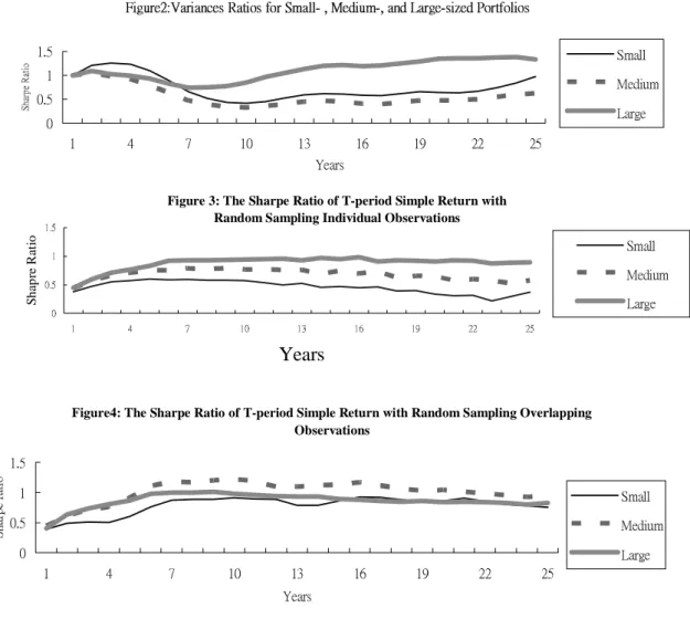
Figure 2 shows that, with the lengthening of the holding period, the variance ratios rise first, then decline,
2
and eventually increase for all portfolios. Specifically, for the small-sized portfolio the variance ratio reaches the top on the third year, declines afterwards, and reverts to an upward trend for horizons longer than ten years. This suggests that returns on the small-sized portfolio are positively autocorrelated in the short term, but the trend is reversed afterwards. For medium- and large-sized portfolios, the variance ratios also have the same pattern as the small-size portfolios. The result confirms the literature that smaller-sized portfolios are riskier than large-sized portfolio in the short term. Surprisingly, however, the result in Figure 2 indicates that large-sized portfolio may become riskier for investment horizons longer than ten years because of the stronger positive higher-order autocorrelations. Since returns are serial correlated, it is not surprising that the ranking of the Sharpe measures of an asset will differ when data of different intervals are used. The results in Figure 2 also indicate that when investment horizons are lengthened long enough (e.g., seven years for large portfolios and ten years for medium and small portfolios), long-term investment does bear relatively lower risk. This confirms the conventional wisdom that the risk in the long-term investment is relatively lower, and suggests that the markets overreact and depict mean-reverting phenomenon (e.g., Fama and French, 1988; Poterba and Summers, 1988).3
To compute the Sharpe ratios for various lengths of horizon, simulation is used here to generate sample return distributions for portfolios of small, medium, and large stocks for holding periods from one year to twenty-five years. For comparison purposes, we calculate the Sharpe ratios based on block sampling and independent sampling as well.
Figure 3 plots the Sharpe ratios for the three portfolios based on independent sampling. Specifically, for a given holding period, say T, we generate a sample of T-period returns for each portfolio by randomly selecting T historical annual returns with replacement and compute the compounded return. For example, consider the case of the small-stock portfolio with a three-year investment horizon. Three annual returns are selected at random from the historical returns over the 1927-2001 period, and then a three-year holding period return is computed using equation (3). This process is then repeated 5,000 times, yielding a sample of 5,000 portfolio returns for each holding period. Then, the T-period Sharpe ratio can be calculated based on the sample estimates of mean and variance of the artificial sample. Since returns are generated independently, the time-series pattern embedded in the original series is broken down, and the procedure generates independent returns. Indeed, from Figure 3 it can be seen that the shapes of the variance ratios are similar to the one plotted in Figure 1. This is not surprising because independent sampling eliminates all serial dependency in the data. Another interesting finding in Figure 3 is that the ranking of the portfolios remains the same through all horizons. This is also expected for the same reason. Clearly, such a result is entirely driven by the independent nature of the simulation.
To avoid the above problem (independent resampling breaks the time-series pattern and generates independent returns), we redo the analysis based on block sampling to capture the dependency in the data. Specifically, for a k-period holding horizon, we first randomly pick a year, say q, between 1927 and (2001-k+1) with each year being selected with equal probability, and then pick R(q,q+k-1) as a k-period holding return. This retains the time-series property within the return. Then we repeat the procedure 5,000 times and compute the excess mean and standard deviation of the 5,000 returns. Dividing the excess mean by standard deviation, we get the Sharpe ratio.4
Figure 4 presents the result based on block sampling. Unlike the finding from independent resampling, the result in Figure 4 indicates that with block resampling the length of the investment horizon becomes relevant. Moreover, with block data, the Sharpe ratio for each portfolio also first increases and then decreases as the holding period is extended. For example, the Sharpe ratio for small-sized portfolio (medium, large) goes up the peak at the horizon of about ten (ten, nine) years, and then decreases gradually afterwards. Although the Sharpe ratios still retain an anti-U shape as in Figure 3, the ranking of portfolios' performance changes as the investment horizon lengthens. For example, the large-sized portfolio performs the best when investment horizon is less than four years, yet becomes dominated by the medium-sized portfolios when holding periods are lengthened to five years or more.5 This indicates that the Sharpe performance measure computed based on
3
One implication is that funds with different time-series properties of investment strategies (e.g., momentum or mean reversion) cannot be evaluated based on the same investment horizon.
4
Here we follow the literature on variance ratio (e.g., Lo and MacKinlay (1988)) that uses overlapping data to improve the performance of statistics in finite-samples.
5
Hodges, Taylor and Yoder (1997) find that large common stocks consistently outperform small stocks when returns are sampled independently.
independent resampling is inappropriate when returns are serially correlated. If asset returns are serially correlated and we estimated the return volatility using independent sampling, we may obtain incorrect ranking in performance, and make wrong asset allocation decision. Besides, recall that the medium-sized portfolio has the lowest variance ratio and the highest Sharpe ratio for longer holding periods. Therefore, the medium-sized portfolio appears to be more attractive for long-term investment.
Figure 3: The Sharpe Ratio of T-period Simple Return with Random Sampling Individual Observations
0 0.5 1 1.5 1 4 7 10 13 16 19 22 25
Years
Sh ap re R at io Small Medium LargeFigure1:The Sharpe Ratio of Simple Return and Investment Horizon under Normal Distribution (Take Mean=0.01 and Standard Deviation=0.25 for Example)
0 0.1 0.2 0.3 0.4 1 11 21 31 41 51 61 71 81 91 Investment horizon Sh ar pe R at io
Figure2:Variances Ratios for Small- , Medium-, and Large-sized Portfolios
0 0.5 1 1.5 1 4 7 10 13 16 19 22 25 Years Sh ar pe R at io Small Medium Large
Figure4: The Sharpe Ratio of T-period Simple Return with Random Sampling Overlapping Observations 0 0.5 1 1.5 1 4 7 10 13 16 19 22 25 Years Sh ar pe ra tio Small Medium Large
4. Conclusions
In this paper, we propose the use of block resampling to obtain proper estimates of Sharpe ratio for various investment horizons. Using block resampling retains the compounding effect in calculating long-term returns and the time-series dependency in the data. We find that rankings based on the Sharpe ratio vary substantially with the investment horizon. In contrast, investment horizons are irrelevant when the estimation of Sharpe ratio is based on independent sampling.
Because investors differ in their risk attitudes and in holding horizons, it is unreasonable to evaluate portfolio performance based on one single investment horizon. Practical implementation of the Sharpe ratio is reasonable only if the intended investment horizon equals to the holding period of the returns used to compute the ratio. However, many investment companies report Sharpe ratio only based on the returns for a fixed investment horizon (e.g., monthly or annual returns). A graph of Sharpe ratio against the investment horizon may be more appropriate for investors with multiyear investment horizons. The Sharpe performance rankings based on short return will be valid only for short-term investors, but not for long-term investors.
References
Bodie, Z., A. Kane, and A.J. Marcus (2002), Investments, 5th edition, Boston: McGraw-Hill Inc.
Chen, S., and C. Lee (1981), The Sampling Relationship Between Sharpe's Performance Measure and its Risk Proxy: Sample Size, Investment Horizon and Market Conditions, Management Science, 27, 607-618.
Chen, S., and C. Lee (1986), The Effects of the Sample Size, the Investment Horizon and Market Conditions on the Validity of Composite Performance Measures: A Generalization, Management Science, 32, 1410-1421.
Fama, F. and K.R. French (1988), Permanent and Temporary Components of Stock Prices, Journal of Political Economy, 96, 246-273.
Gunthorpe, Deborah and H. Levy (1994), Portfolio Composition and the Investment Horizon, Financial Analyst Journal, 50, Jan.-Feb.51-56.
Hodges, Charles W., Walton R.L. Taylor, and James A. Yoder (1997), Stock, Bonds the Sharpe Ratio, and the Investment Horizon, Financial Analysts Journal, 53, Nov.-Dec. 74-80.
Johnson, N. L. and Kotz, S. (1972), Distributions in Statistics: Continuous Multivariate Distributions, New York: John Wiley and Sons.
Levy H. (1972), Portfolio Performance and the Investment Horizon, Management Science, 18, 645-653. Levy H. (1981), The CAPM and the Investment Horizon, Journal of Portfolio Management, 7, 32-40.
Levy H. (1984), Measuring Risk and Performance Over Alternative Investment Horizons, Financial Analyst Journal, 40, 61-68.
Levy H., and Paul A. Samuelson (1992), The Capital Asset Pricing Model with Diverse Holding Periods, Management
Science, 38, 1529-1542.
Lo, A.W. and A.C. MacKinlay (1988), Stock Prices do not Follow Random Walks: Evidence from a Simple Specification Test, Review of Financial Studies, 1, 515-528.
Lo, Andrew (2002), The Statistics of Sharpe Ratios, Financial Analysts Journal, 58, July-August 36-52.
Poterba, J.M. and L.H. Summers (1988), Mean-Reversion in Stock Prices Evidence and Implications, Journal of Financial
Economics, 22, 27-59.
Sharpe, W.F. (1994), The Sharpe Ratio, The Journal of Portfolio Management, 49, 49-58.
Tobin, J. (1965), The Theory of Portfolio Selection, The Theory of Interest Rates, 3-51, edited by F. H. Hahn and F. P. R. Brechling. London: Macmillan.