A Crossover-Imaged Clustering Algorithm with Bottom-up Tree Architecture
CHUNG-I CHANG
Department of Information Management
St. Mary’s Medicine, Nursing and Management
College
100, Lane265, Sec.2, SansingRoad,
Sansing Township, Yilan County 266
TAIWAN
NANCY P. LIN
Department of Computer Science and
Information Engineering
Tamkang University
151 Ying-chuan Road Tamsui, Taipei County
TAIWAN
Abstract
The grid-based clustering algorithms are efficient with low computation time, but the size of the predefined grids and the threshold of the significant cells are seriously influenced their effects. The ADCC [1] and ACICA+ [2]
are two new grid-based clustering algorithms. The ADCC algorithm uses axis-shifted strategy and cell clustering twice to reduce the influences of the size of the cells and inherits the advantage with the low time complexity. And the ACICA+ uses the crossover image of significant cells
and just only one cell clustering. But the extension of original significant cell in one crossover image is not easy to find what else clusters it belongs to. The Crossover-imaged Clustering Algorithm with Bottom-up Tree Architecture, called CIC-BTA, is proposed to use bottom-up tree architecture to have the same results. The main idea of CIC-BTA algorithm is to use the bottom-up tree architecture to link the significant cells to be the pre-clusters and combine pre-pre-clusters into one by using semi-significant cells The final set of clusters is the result.
1. Introduction
Up to now, many clustering algorithms have been proposed [1, 2, 3, 4, 5, 6, 7, 8, 9, 10, 11, 12, 13, 14, 15], and generally, the called grid-based algorithms are the most computationally efficient ones. The main procedure of the grid-based clustering algorithm is to partition the data space into a finite number of cells to form a grid structure, and next, find out the significant cells whose densities exceed a predefined threshold, and group nearby significant cells into clusters finally. Clearly, the grid-based algorithm performs all clustering operations on the generated grid structure; therefore, its time complexity is only dependant on the number of cells in each dimension of the data space. That is, if the number of the cells in each dimension can be controlled as a small value, then the time complexity of the grid-based algorithm will be low. Some famous algorithms of the grid-based
clustering are STING [13], WaveCluster [14], CLIQUE [15], and ADCC [1] and ACICA+ [2].
In general, grid-based clustering algorithm is one of the most computationally efficient algorithms, and the ACICA+ uses the crossover image of significant cells and
just only one cell clustering. But the extension of original significant cell in one crossover image is not easy to find what else clusters it belongs to. To fix the problem of not easy finding clusters, we propose a new grid-based clustering algorithm which is called the Crossover-Imaged Clustering Algorithm with Bottom-up Tree Architecture, CIC-BTA, in this paper.
The main idea of our proposed CIC-BTA is to utilize tree architecture, three types of significant cells and two layers, connection and combination, to identify the set of clusters.
The rest of the paper is organized as follows: In section 2, some popular grid-based clustering algorithms are mentioned again. In section 3, our proposed clustering algorithm, CIC-BTA algorithm, is introduced. In section 4, an experiment and some discussions are displayed. Section 5 is the conclusion.
2. Grid-based clustering algorithm
Grid-based clustering algorithm is an efficient clustering algorithm, and three famous grid-based clustering algorithms are NSGC [11], and ADCC [1] and ACICA+ [2].
The NSGC (A new shifting grid clustering algorithm) (Ma et al., 2004), using the concept of shifting grid. The algorithm is a non-parametric type, which does not require users inputting parameters. It divides each dimension of the data space into certain intervals to form a grid structure in the data space. Based on the concept of sliding window, shifting of the whole grid structure is introduced to obtain a more descriptive density profile. It clusters data in a way of cell rather than in points.
The idea of ADCC (Adaptable Deflect and Conquer Clustering) (Lin et al., 2007) is to utilize the predefined
grids and predefined threshold to identify the significant cells, by which nearby cells that are also significant can be merged to develop a cluster in the first place. Next, the modified grids which are deflected to half size of the grid are used to identify the clusters again. Finally, the new generated clusters and the initial clusters are merged to be the final clustering result.
The ACICA+ (the Axis-shifted Crossover-Imaged Clustering algorithm) (Lin et al., 2007) uses the crossover image of significant cells and just only one cell clustering. It also is to reduce the influences of the size of the predefined grids and the threshold of the significant cells. In ACICA+, the extension of original significant cell in one crossover image is not easy to find what else clusters it belongs to. The Crossover-imaged Clustering Algorithm with Bottom-up Tree Architecture, called CIC-BTA, is proposed to use bottom-up tree architecture to have the same results. It uses the bottom-up tree architecture to link the cells in the cluster and combine pre-clusters to be the final results.
3. CIC-BTA algorithm
Though the ACICA+ uses the crossover image of
significant cells and just only one cell clustering, the extension of original significant cell in one crossover image is not easy to find what else clusters it belongs to. To improve the chief problem, the CIC-BTA algorithm, Crossover-imaged Clustering Algorithm with Bottom-up Tree Architecture, further links cells in the same cluster and combines pre-clusters into one. The CIC-BTA generates the final clustering results the same with ADCC and ACICA+. The root of the bottom-up tree is the whole
database grouped into the set of clusters.
For CIC-BTA, it uses a bottom-up tree architecture to fix the problem of cater-corner significant cells, the extension of original significant cell in one crossover image is not easy to find what else clusters it belongs to. Here, we have some definition of cell at first.
Definition1. Significant cell
If the density of cell X is greater than or equal to a minimum threshold μ, then the cell X is called Significant cell.
Definition2. Close-nearby cell and Open-nearby cell The n-dimensional grid-based databases are partitioned into kn cells with same size. Close-nearby(X)={Y| X∩Y > one point }, which is mean that intersection is one side of cell X and Y. Open-nearby(X)={Y| X∩Y = one point }, which is mean that intersection is one corner point of cell X and Y.
Definition3. Semi-Significant cell
The n-dimensional grid-based databases are
partitioned into kn cells with same size to be the original
grid structure, G1. The original coordinate origin is next
shifted by distance
d
in each dimension of the data space to generate the second grid structure, G2, so that thecoordinate of each point becomes
d
less in each dimension.Semi-significant cell X ={X | X∩Y ≠φ,X∩Z ≠φ,X
∉
significant(G1),
∃
Y,Z∈
significant(G2), Z∈
Close-nearby(Y) }
If the cell X in G1 is not a significant cell and its
crossover image belongs to at least two Close-nearby cells in grid structure G2, then X is called Semi-significant cell.
Definition4. Non-Significant cell
For n-dimensional original grid structure, G1, its
original coordinate origin is shifted to generate the second grid structure, G2.
Non-significant cell X ={X | X ∩ Y ≠ φ ,X ∩ Z ≠ φ ,X
∉
significant(G1),∃
Y,Z∈
significant(G2),∀
Z∉
Close-nearby(Y) }
If the cell X in G1 is not a significant cell and its
crossover image belongs to some Close-nearby cells in grid structure G2, then X is called Semi-significant cell.
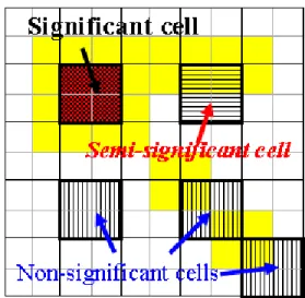
Then the three types of significant cells are shown in figure 1.
Figure 1. Three types of significant cells
Then, the clusters will be generated from the same crossover image by using ACICA+. But the extension of
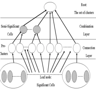
original significant cell in one crossover image is not easy to find what else clusters it belongs to. In CIC-BTA, the clustering tree is built and shown in figure 2.
Figure 2. Clustering trees (CT)
The significant cell X and its extension are connected to be one leaf node of clustering Tree (CT). In connection layer of CT, connect the significant cells to be the pre-clusters, sub-trees of CT. And in combination layer, use semi-significant cells to combine pre-clusters to be the final clustering results, the root of CT. The procedure of CIC-BTA is shown in the following steps.
Step 1: Generate the second grid structure.
By dividing into k equal parts in each dimension, the n dimensional data space is partitioned into kn
non-overlapping cells to be the grid structure G2.
Step 2: Identify the significant cells.
Next, the density of each cell is calculated to find out the image of significant cells whose densities exceed a predefined threshold.
Step 3: Transform the new grid structure.
The second grid structure is next shifted by distance
d
in each dimension of the data space to generate the first grid structure, G1.Step 4: Identify significant and semi-significant cells. Next, the density of each cell is calculated to find out the new image of significant cells whose densities exceed a predefined threshold. And if the cell X in G1 is not a significant cell and its
crossover image belongs to at least two Close-nearby cells in grid structure G2, then
Semi-significant cell X is found. The semi-Semi-significant cell is the area can combine two connected clusters, which are close-nearby cells in G2 but not
significant in G1, into one, shown in figure 1.
Step 5: connect the significant cells to generate the pre-clustering results.
{
2j 1i 2j 2j 2}
1i
i
{C
}
C
|
C
C
,
C
SC
CEXT
=
∪
∩
≠
φ
∈
The image of significant cells in G2 is generated
and projected on the original grid structure to be the crossover image. The significant cell in first grid structure and its crossover image are combined to be the extension of significant cell (CEXT). In the connection layer, the nearby significant cells are connected into one cluster. And one example of cater-corner significant cell in G2 is existed, shown in figure 3. Next, the two
significant open-nearby cells in G1 have to be
connected into one cluster by the cater-corner significant cell in G2, which is the intersection of
extension of the two significant open-nearby cells in G1. Then, the pre-clustering results are built.
The significant cell X and its extension is the node of clustering Tree (CT) and the pre-clustering results are sub-tree of CT.
Figure 3. Cater-corner significant cell
Step 6: Combine semi-significant cells and other significant cells in G2 to generate the final
clustering result.
At first, combine clustering results by using semi-significant cells to combine pre-clustering results. to be the final clustering results. Then the whole set of clusters is the root of CT.
4. Experiments
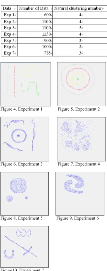
Here, we experiment with seven different data shown in figure 4. ~ figure 10. And the features are presented in Table 1.
Figure 4. Experiment 1 Figure 5. Experiment 2
Figure 6. Experiment 3 Figure 7. Experiment 4
Figure 8. Experiment 5 Figure 9. Experiment 6
Figure10. Experiment 7
In Figure11, it shows the correct rates of CIC-BTA and CLIQUE, where the correct clustering result of CLIQUE is by using one of original or new grid structures in the experiment. The correct rates of CIC-BTA are all
higher than CLIQUE. In the experiment, the correct rates comparison is by using random 100 sets of parameters (density threshold, number of dividing parts in each dimension) from (1,16) to (3,55).
Figure 11. Correct rates of CIC-BTA and CLIQUE
5. Conclusion
The algorithm we proposed, the Crossover-Imaged Clustering Algorithm with Bottom-up Tree Architecture, CIC-BTA algorithm, uses three types of significant cells and two layers to generate the clustering results, which makes the important contribution to support the obvious wider ranges of size of the cell and threshold of the density to reduce the drawbacks of grid-based clustering algorithms. And the clustering results of CIC-BTA are exactly the same as the results of ACICA+ and the number of cell-clustering times has just only once, too. So it is fast and simple to realize that the CIC-BTA algorithm also inherits the advantage with the low time complexity.
10. References
[1] N. Lin, C. Chang, and C. Pan. “An Adaptive Deflect and Conquer Clustering algorithm”, In Proc. of 6th WSEAS Int. Conf. ACOS’07, 2007, pages 156-160.
[2] N. Lin, C. Chang,” An Axis-shifted Crossover-Imaged Clustering Algorithm”, In Proc. of 7th WSEAS Int. Conf. SMO’07, 2007, pages 213-218
[3] J. MacQieen. Some methods for classification and analysis of multivariate observation. Proc. 5th Berkeley Symp. Math. Statist, Prob., 1:281-297,1967
[4] L. Kaufman and P.J. Rousseeuw. Finding Groups in Data: An Introduction to Cluster Analysis. New York: John Wiley & Sons, 1990.
[5] Charu C. Aggarwal, Philip S. Yu, “An effective and efficient algorithm for high-dimensional outlier detection”
[6] M. Ester, H. Kriegel, J. Sander, and X. Xu. “A Density-Based Algorithm for Discovering Clusters in Large Spatial Databases with Noise”, In Proc. of 2nd Int. Conf. on KDD, 1996, pages 226-231.
[7] A. Hinneburg and D. A. Keim,. “An Efficient Approach to Clustering in Large Multimedia Databases with Noise”, In Knowledge Discovery and Data Mining, 1998, pages 58-65.
[8] ANKERST M. etc. “OPTICS: Ordering Points to Identify the Clustering Structure.” In Proc. ACM SIGMOD Int. Conf. on MOD, 1999, pages 49-60.
[9] A. H. Pilevar, M. Sukumar, “GCHL: A grid-clustering algorithm for high-dimensional very large spatial data bases”, Pattern Recognition Letters 26(2005), 999-1010 [10] ZHAO Y.C., SONG J.,”GDILC: A Grid-based Density-Isoline Clustering Algorithm.”, In Proc. Internet. Conf. on Info-net, Vol 3, pp.140-145,2001
[11]Ma, W.M., Eden, Chow, Tommy, W.S., “A new shifting grid clustering algorithm”, Pattern Recognition 37 (3),2004,503-514
[12]Alevizos, P., Boutsinas, B., Tasoulis, D., Vrahatis, M.N.,”Improving the K-windows clustering algorithm”,
In Proc. 14th IEEE Internat. Conf. on Tools with Artificial Intell, pp.239-245, 2002.
[13] Wang, Yang, R. Muntz, Wei Wang and Jiong Yang and Richard R. Muntz “STING: A Statistical Information Grid Approach to Spatial Data Mining”, In Proc. of 23rd Int. Conf. on VLDB, 1997, pages 186-195.
[14] G. Sheikholeslami, S. Chatterjee, and A. Zhang. “WaveCluster: a wavelet-based clustering approach for spatial data in very large databases”, In VLDB Journal: Very Large Data Bases, 2000, pages 289-304.
[15] R. Agrawal, J. Gehrke, D. Gunopulos, and P. Raghavan. “Automatic sub-space clustering of high dimensional data for data mining applications”, In Proc. of ACM SIGMOD Int. Conf. MOD, 1998, pages 94-105.