Fe
de
ra
l
R
ese
rve
Ba
n
k of C
hi
cago
Estimation of Panel Data Regression
Models with Two-Sided Censoring
or Truncation
Sule Alan, Bo E. Honoré, Luojia Hu, and
Søren Leth–Petersen
Estimation of Panel Data Regression Models
with Two-Sided Censoring or Truncation
Sule Alany Bo E. Honoréz Luojia Hu x Søren Leth–Petersen {
November 14, 2011
Abstract
This paper constructs estimators for panel data regression models with individual speci…c heterogeneity and two–sided censoring and truncation. Following Powell (1986) the estimation strategy is based on moment conditions constructed from re–censored or re–truncated residuals. While these moment conditions do not identify the parameter of interest, they can be used to motivate objective functions that do. We apply one of the estimators to study the e¤ect of a Danish tax reform on household portfolio choice. The idea behind the estimators can also be used in a cross sectional setting.
Key Words: Panel Data, Censored Regression, Truncated Regression. JEL Code: C20, C23, C24.
This research was supported by NSF Grant No. SES-0417895 to Princeton University, the Gregory C. Chow Econometric Research Program at Princeton University, and the Danish National Research Foundation, through CAM at the University of Copenhagen (Honoré) and the Danish Social Science Research Council (Leth–Petersen). We thank Christian Scheuer and numerous seminar participants for helpful comments. The opinions expressed here are those of the authors and not necessarily those of the Federal Reserve Bank of Chicago or the Federal Reserve System.
yFaculty of Economics, University of Cambridge, Sidgwick Avenue, Cambridge, UK, CB3 9DD. Email: [email protected].
zDepartment of Economics, Princeton University, Princeton, NJ 08544-1021. Email: [email protected]. xEconomic Research Department, Federal Reserve Bank of Chicago, 230 S. La Salle Street, Chicago, IL 60604. Email: [email protected].
{Department of Economics, University of Copenhagen, Øster Farimagsgade 5, Building 26, DK-1353 Copenhagen K. and SFI, The Danish National Centre for Social Research, Herluf Trolles Gade 11, DK-1052. Email : [email protected].
1
Introduction
This paper generalizes a class of estimators for truncated and censored regression models to allow for two–sided truncation or censoring. The class of estimators is based on pairwise comparisons and the proposed generalizations therefore apply to both panel data and cross sectional data.
A leading example of when two–sided censored regression models are useful is when the de-pendent variable is a fraction. For example, Alan and Leth-Petersen (2006) estimate a portfolio share equation where the portfolio shares are between 0 and 1, with a signi…cant number of obser-vations on either of the limits. Other recent applications in economics of regression models with two–sided censoring include Lafontaine (1993), Petersen and Rajan (1994), Petersen and Rajan (1995), Houston and Ryngaert (1997), Fehr, Kirchler, Weichbold, and Gachter (1998), Huang and Hauser (1998), McMillan and Woodru¤ (1999), de Figueriredo and Tiller (2001), Huang and Hauser (2001), Fenn and Liang (2001), Poterba and Samwick (2002), Nickerson and Silverman (2003), Of-…cer (2004), Charness, Frechette, and Kagel (2004), Andrews, Schank, and Simmons (2005) and Gi¤ord and Bernard (2005). We formulate the two–sided censored regression model as observations of (y; x; L; U) from the model
y =x0 +" (1)
wherey is unobserved, but we observe
y= 8 > > > < > > > : L if y < L y if L y U U if y > U (2)
and is the parameter of interest. Whenyis a share,LandU will typically be 0 and 1, respectively. We will focus on panel data settings so the observations are indexed byiand twherei= 1; : : : ; n andt= 1; : : : Ti. This allows for unbalanced panels, but we will maintain the restrictive assumption
that Ti is exogenous in the sense that it satis…es all the assumptions made on the explanatory
variables. In a panel data setting, it is also important to allow for individual speci…c e¤ects in the errors "it. We will do this implicitly by making assumptions of the type that "it is stationary
conditional on(xi1: : : xiTi)or that"itand"isare independent and identically distributed conditional on some unobserved component ist. These will have the textbook speci…cation"it=vi+ it (f itg
i.i.d.) as a special case. In section 4.2, we discuss how to apply the same ideas to construct
estimators of the cross sectional version of the model.
distribution of(y ; x; L; U)conditional onL y U. Two–sided truncated regression models are less common than two–sided censored regression models, but they play a role in duration models. Suppose, for example, that one wants to study the e¤ect of early life circumstances on longevity by linking the Social Security Administration’s Death Master File to the 1900–1930 U.S. censuses1. This will miss a substantial number of deaths: (1) individuals who died under age 65 (since they were less likely to be collecting social security bene…ts and thus their deaths were less likely to be captured); (2) individuals who died before the year 1965 (the beginning of the computerized Social Security …les); and (3) individuals who died after the last year the data is available. This is a case of two-sided truncation because we observe an individual only if the dependent variable, age at death, is greater than 65 years and if the death occurs between 1965 and the last year the data is available. This is essentially the empirical setting in Ferrie and Rolf (2011), although they only consider data from the 1900 census, so right–truncation is unlikely to be an issue in their application.
Honoré (1992) constructed moment conditions for similar panel data models with one–sided truncation or censoring and showed how they can be interpreted as the …rst–order conditions for a population minimization problem that uniquely identi…es the parameter vector, . This paper generalizes that approach to the case when the truncation or censoring is two–sided. The main contribution of the paper is to show that some of those moment conditions can be turned into a minimization problem that actually uniquely identi…es when there is two–sided censoring or truncation. This is an important step because the moment conditions that we derive do not identify the parameters of the model. This is a generic problem with constructing estimators based on moment conditions. For example, Powell (1986) constructed moment conditions for a related cross sectional truncated and censored regression models based on symmetry of the error distribution. He also pointed out that while these moment conditions did not identify the parameter of interest, minimization of an objective function based on them did lead to identi…cation.
The rest of the paper is organized as follows. Section 2 derives the moment conditions and the associated objective function for models with two–sided censoring and two–sided truncation. Sec-tion 3 then discusses how these can be used to estimate the parameters of interest. GeneralizaSec-tions of the two models considered in Section 2 are discussed in Section 4. We present the empirical application in Section 5 and Section 6 concludes.
2
Identi…cation: Moment Conditions and Objective Functions
The challenge in constructing moment conditions in models with censoring and truncation is that one typically starts with assumptions on " conditional on x in (1). If one had a random sample of (y ; x) then these assumptions could be used immediately to construct moment conditions. For example if E["x] = 0, then one has the moment conditions E[(y x0 )x] = 0. However withtruncation or censoring,y x0 will not have the same properties as". The idea employed in Powell (1986), Honoré (1992) and Honoré and Powell (1994) is to apply additional censoring and truncation to y x0 in such a way that the the resulting re–censored or re–truncated residual satis…es the conditions assumed on". For example, Powell (1986) assumed that"is symmetric conditional on x in a censored regression model with censoring from below at 0. If that is the case, then y x0 = maxf"; x0 gwill clearly not be symmetric conditional on x, but the re–censored residuals,
minfy x0 ; x0 gwill be. This implies moment conditions of the typeE[minfy x0 ; x0 gx] = 0. Unfortunately, this moment condition will not in general identify , but Powell (1986) was able to prove that the integral (as a function of b) of E[minfy x0b; x0bgx] is uniquely minimized at b = under appropriate regularity assumptions. Honoré (1992) applied the same insight to a panel setting where the assumption was that " is stationary conditional on the entire sequence of explanatory variables. Again, censoring or truncation destroys this stationarity, but it can be restored for a pair of residuals by additional censoring. Honoré and Powell (1994) then applied the same idea to any pair of observations in a cross section, and Hu (2002) generalized it to allow for lagged latent dependent variables as covariates.
The contribution of this paper is to generalize the approach in Honoré (1992) to the case with two–sided censoring or truncation. As in Powell (1986), Honoré (1992) and Honoré and Powell (1994), it is straightforward to construct moment conditions based on some re–censored or re–truncated residuals. However, it is not clear that these moment conditions will identify the parameters of interest, and we therefore construct (population) objective functions from these moment conditions, and then explicitly verify that these objective functions are uniquely minimized at the parameter. It is the construction of the objective functions and verifying that they are uniquely minimized at the true parameter value that constitute the methodological contribution of the paper.
The general approach is to start with a comparison of two observations for a given individual in a panel. Based on these observations we will construct re–censored or re–truncated residuals
eits(yit; xit; xis; Lit; Lis; Uit; Uis; b) andeist(yis; xis; xit; Lit; Lis; Uit; Uis; b)that have the same
prop-erties as"it and"iswhen b= . This will then imply that if"it and "is are identically distributed
conditional on(xit; xis), then
E[ (eits(yit; xit; xis; Lit; Lis; Uit; Uis; ) eist(yis; xis; xit; Lit; Lis; Uit; Uis; ))jxit; xis] = 0: (3)
This will form the basis for construction of our estimators. Of course, once it has been established that eits(yit; xit; xis; Lit; Lis; Uit; Uis; ) and eist(yis; xis; xit; Lit; Lis; Uit; Uis; ) are identically
dis-tributed then for any function, ( ), we also have the moment condition
E[ ( (eits(yit; xit; xis; Lit; Lis; Uit; Uis; )) (eist(yis; xis; xit; Lit; Lis; Uit; Uis; )))jxit; xis] = 0:
(4) provided that the moment exists.
Moreover, if the errors "it and "is are also independent conditional on (xit; xis), then so are
eits(yit; xit; xis; Lit; Lis; Uit; Uis; ) and eist(yis; xis; xit; Lit; Lis; Uit; Uis; ). This implies that their
di¤erence is symmetrically distributed around 0, so for any odd function ( ),
E[ ( (eits(yit; xit; xis; Lit; Lis; Uit; Uis; ) eist(yis; xis; xit; Lit; Lis; Uit; Uis; )))jxit; xis] = 0: (5)
provided that the moment exists.2
In this paper we will focus on (3) and the generalization (5). The reason for this is that in a linear model without censoring or truncation, (3) will correspond to OLS on the di¤erenced data, whereas (5) will also accommodate least absolute deviation estimation on the di¤erenced data as a special case. As already mentioned, the construction of the residualseits(yit; xit; xis; Lit; Lis; Uit; Uis; ) is
fairly straightforward, and the challenge is to show that although (3) and (5) may not identify , and unconditional version of them can be integrated to yield a population objective function that is uniquely minimized at b = . This will involve the integral of ( ), which we will denote by
( ), and in addition to being odd, we will assume that ( )is also increasing, so ( ) is a convex symmetric function. The leading cases are (d) =jdjand (d) =d2.
In order to simplify the exposition, we will …rst develop the case when Lit= 0and Uit= 1. We
will then demonstrate that the result can be adapted to the general case.
2Of course one could combine the insight in (4) and (5) to get even more general moment conditions. See also the
2.1 Two–Sided Censoring
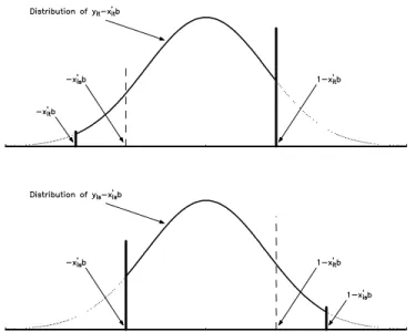
Consider …rst the situation with two–sided censoring. Consider an individual,i, in two time periods, t ands, and assume that "it and"is are identically distributed. The distribution ofyit x0it will
be the same as that of "it except that the former is censored from below at x0it and from
above at 1 x0it . Figure 1 illustrates this. The dotted line depicts the distribution of "it, while
the solid line gives the distribution of yit x0it , which typically has point mass at x0it and
1 x0it (illustrated by the fatter vertical lines). Since x0it will typically di¤er from x0is , the distributions of yit x0it and yis x0is (given (xit; xis)) will di¤er even if f"itg is stationary
(given (xit; xis)). However, it is clear that one could obtain identically distributed “residuals” by
arti…cially censoringyit x0it and yis x0is from below atmaxf x0it ; x0is gand from above at
minf1 x0
it ;1 x0is g. See the dashed lines in Figure 1. One can then form moment conditions
from the fact that the di¤erence in these “re–censored”residuals will be orthogonal to functions of
(xit; xis).3 Of course, this construction is only useful if 1< x0it x0is <1, because otherwise,
the supports of yit x0it and yis x0is will not overlap.
In order to proceed, we need explicit expressions for the di¤erence in these “re–censored”resid-uals. Consider …rst the case when x0it x0is . Then the di¤erence in the arti…cially censored residuals for individualiin periods tand sis
max yit x0it ; x0is min yis x0is ;1 x0it (6) = max yit x0it x0is ;0 xis0 min yis;1 x0it x0is x0is = max yit x0it x0is ;0 min yis;1 x0it x0is ; and when x0it x0is min yit x0it ;1 x0is max yis x0is ; x0it (7) = min yit;1 + x0it x0is x0it max yis+ x0it x0is ;0 x0it = min yit;1 + x0it x0is max yis+ x0it x0is ;0 :
3Clearly, one can also use the fact that di¤erences in functions of the re–censored residuals will be orthogonal to
functions for the explanatory variables. As discussed in Arellano and Honoré (2001), one can also construct moment conditions based on symmetry under the additional assumption that ("i1; :::; "iT) is exchangeable conditional on
Figure 1: Illustration of Re–Censored Residuals when x0it > x0is . If we de…ne u(y1; y2; d) = 8 > > > > > > > > > > > > > > > < > > > > > > > > > > > > > > > : 0 for d < 1 1 +d for 1< d < c1
minf1 y2; y1g for c1 < d < c2 y1 y2 d for c2 < d < c3
maxfy1 1; y2g for c3 < d < c4 d 1 for c4 < d <1
0 for d >1
(8)
wherec1= minf y2; y1 1g,c2 = maxf y2; y1 1g,c3 = minf1 y2; y1gandc4 = maxf1 y2; y1g thenu(yit; yis; x0it x0is )will give the di¤erence in the re–censored residuals discussed above (see
Appendix 1). Hence the moment conditions are
E u yit; yis; x0it x0is xit; xis = 0;
which implies the unconditional moments
E u yit; yis;(xit xis)0 (xit xis) = 0: (9)
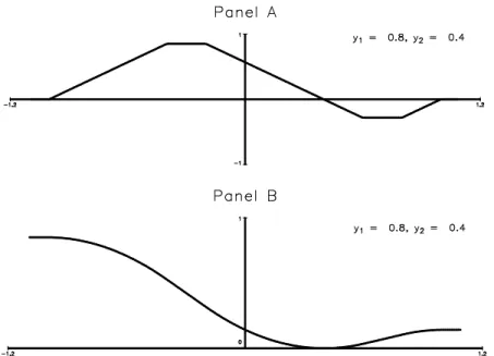
Panel A of Figures 2–4 depict the contribution to the moment condition function u(y1; y2; d)
Figure 2: The Functionsu(y1; y2; ) and U(y1; y2; ). Neither Observation Censored.
observation (Figure 3) and pairs with one observation censored from above and one from below (Figure 4).
Although the true parameter value will satisfy (9), it is not in general the unique solution to the moment condition. This is illustrated in Panel A of Figure 5. It considers the case when yi1 N(0:5;1)and yi2 N(0:4;1) and both are censored from below at 0 and from above at 1. Note that this is the data generation process that one would get with = 0:1,xi1 = 1 andxi2 = 0 for all i.
It is clear from Figure 5 that the moment condition E[u(yit; yis; x0itb x0isb)jxit; xis] = 0 does
not identify the parameter, , of the model. The most obvious reason is that, as mentioned, only observations for which 1 < (xi1 xi2)0b < 1 will contribute. In this case xi1 xi2 = 1 for all observations, so the moment condition is automatically satis…ed whenjbj>1.
Following Powell (1986), we attempt to overcome the non–identi…cation based on the moment condition by turning it into the …rst order condition for a minimization problem. It is easy to see that (9) is (half of minus) the …rst order condition for minimizing
Figure 3: The Functionsu(y1; y2; )and U(y1; y2; ). One Observation Censored.
Figure 5: The FunctionsE[u(y1; y2; )]and E[U(y1; y2; )]. where U(y1; y2; d) = 8 > > > > > > > > > > > > > > > < > > > > > > > > > > > > > > > : 1 + 2c1+c21 2c3c1+ 2c3c2+ (y1 y2 c2)2 for d < 1 2d d2+ 2c1+c21 2c3c1+ 2c3c2+ (y1 y2 c2)2 for 1< d < c1 2c3d+ 2c3c2+ (y1 y2 c2)2 for c1< d < c2 (y1 y2 d)2 for c2< d < c3 2c2d+ 2c2c3+ (y1 y2 c3)2 for c3< d < c4 d2+ 2d+c24 2c4 2c2c4+ 2c2c3+ (y1 y2 c3)2 for c4< d <1 1 +c2 4 2c4 2c2c4+ 2c2c3+ (y1 y2 c3)2 for d >1 :
Panel B of Figures 2–4 depict the contribution to the objective function U(y1; y2; d) for pairs of uncensored observations (Figure 2), pairs with one censored and one uncensored observation (Figure 3) and pairs with one observation censored from above and one from below (Figure 4). Like the estimator for the panel data one–sided censored regression model developed in Honoré (1992), the objective function is piecewise quadratic or linear. However, surprisingly, going from one–sided to two–sided censoring ruins the convexity of the objective function, and the shape of the function is more similar to the objective function in Powell (1986) although that estimator was developed for a cross section model with symmetrically distributed errors.
minimizing the population objective function in (10). However, sinceU is constant, linear, quadratic and convex, and quadratic and concave over di¤erent regions, it is not at all obvious that will be the unique solution to these …rst order conditions. The key step for establishing identi…cation of is therefore to establish that the function in (10) is minimized at . We establish this in Appendix 1 (Section 7.1), and the result is illustrated in Panel B of Figure 5.
As mentioned, it is also possible to construct moment conditions based on (5). Let be convex and symmetric, and let ( ) = 0( ) (when it exists). When "it and "is are independent and
identically distributed, we also have the moment conditions
E u yit; yis; x0it x0is xit; xis = 0
which imply the unconditional moments
E u yit; yis;(xit xis)0 (xit xis) = 0 (11) where (u(y1; y2; d)) = 8 > > > > > > > > > > > > > > > < > > > > > > > > > > > > > > > : 0 for d < 1 (1 +d) for 1< d <minf y2; y1 1g=c1 (c3) for c1< d <maxf y2; y1 1g=c2 (y1 y2 d) for c2< d <minf1 y2; y1g=c3 (c2) for c3 < d <maxf1 y2; y1g=c4 (d 1) for c4< d <1 0 for d >1
Except for a multiplicative constant, (11) is the …rst order condition for minimizing
E U yit; yis;(xit xis)0b (12)
whereU is found by integrating (u(y1; y2; d))over each of the regions and insisting on continuity at the boundaries between the regions:
U (y1; y2; d) = 8 > > > > > > > > > > > > > > > < > > > > > > > > > > > > > > > : (0) (1 +c1) (c3)c1+ (c3)c2+ (y1 y2 c2) for d < 1 (1 +d) (1 +c1) (c3)c1+ (c3)c2+ (y1 y2 c2) for 1< d < c1 (c3)d+ (c3)c2+ (y1 y2 c2) for c1 < d < c2 (y1 y2 d) for c2 < d < c3 (c2)d+ (c2)c3+ (y1 y2 c3) for c3 < d < c4 (d 1) (c4 1) (c2)c4+ (c2)c3+ (y1 y2 c3) for c4 < d <1 (0) (c4 1) (c2)c4+ (c2)c3+ (y1 y2 c3) for d >1 :
2.2 Two–sided Truncation
Mimicing the argument for the model with two–sided censoring, it is clear that if "it and "is are
independent and identically distributed conditional on(xit; xis), then the observed errors,yit x0it ,
will be i.i.d. except that the sampling scheme will have truncated them at di¤erent points, x0it and x0is from below and 1 x0it and 1 x0is from above. We can then construct identically distributed residuals by arti…cially truncating yit x0it at x0is from below and at1 x0is from
above (and similarly for yis x0is ). This yields many moment conditions, including
E r yit; yis;(xit xis)0 E yit yis (xit xis)0 1 x0is yit x0it 1 x0is
1 x0it yis x0is 1 x0it (xit xis) (13)
= 0
It is an easy exercise to see that except for a multiplicative constant (13) is the …rst order condition for minimizing
E R yit; yis;(xit xis)0b (14) whereR(y1; y2; d) is de…ned by 8 > > > < > > > : 1 2(y1 y2 maxfy1 1; y2g) 2 if max fy1 1; y2g> d 1 2(y1 y2 d) 2 if max fy1 1; y2g d minfy1;1 y2g 1 2(y1 y2 minfy1;1 y2g) 2 if d >min fy1;1 y2g
Figure 6 depicts the functionR and its derivative, whereas Figure 7 shows their expectation when y1 N(0:5;1)and y2 N(0:4;1)and both are truncated from below at 0 and from above at 1.
More generally, again let be convex and symmetric, and let ( ) = 0( ) (when it exists). Then E yit yis (xit xis)0 1 x0is yit x0it 1 x0is 1 x0it yis x0is 1 x0it (xit xis) = 0 or E yit yis (xit xis)0 1 0 yit (xit xis)0 1 1 0 yis+ (xit xis)0 1 (xit xis) = 0
Figure 6: The Functions r(y1; y2; ) andR(y1; y2; ).
or with = (xit xis)0 ,
0 = E[ (yit yis ) 1f0 yit 1g 1f0 yis+ 1g(xit xis)]
= E[ (yit yis ) 1f0 yit g 1fyit 1g 1f0 yis+ g 1fyis+ 1g(xit xis)]
= E[ (yit yis ) 1f yitg 1fyit 1 g 1f yis g 1f 1 yisg(xit xis)]
= E[ (yit yis ) 1fmaxfyit 1; yisg minfyit;1 yisgg(xit xis)]
This is minus the derivative ofE R yit; yis;(xit xis)0b evaluated atb= , where
R (y1; y2; d) = 8 > > > < > > > :
(maxfy1 1; y2g) for d <maxfy1 1; y2g
(y1 y2 d) for maxfy1 1; y2g d minfy1;1 y2g
(minfy1;1 y2g) for d >minfy1;1 y2g
As was the case for the censored model, the argument above only establishes that the true will solve the …rst order condition for minimizing E R yit; yis;(xit xis)0b . On the other
hand, it is clear that without additional strong assumptions, will not be the unique minimizer. The reason is that we know that, in general, the truncated regression model will not be identi…ed with exponentially distributed errors. As a result, assumptions must be added that rule out the exponential distribution. In Appendix 1 (section 7.2), we show that is the unique minimizer of E R yit; yis;(xit xis)0b , and more generally ofE R yit; yis;(xit xis)0b , provided that the
errors have a log–concave probability distribution.
3
Estimation
The arguments leading to identi…cation of the parameters of interest, , above were based on comparing two observations for the same individual and we showed that could be expressed as the unique minimizer of an expectation of the form E Q yit; yis;(xit xis)0b for some function
Q. This suggests estimating by minimizing a sample analog of this such as
b= arg min b 1 n n X i=1 Ti 2 1 X 1 s<t Ti Q yit; yis;(xit xis)0b
In this aggregation, observations get di¤erent weight depending on the number of observations for a given individual. Alternatively, one could also use objective functions of the type
arg min b 1 n n X i=1 X 1 s<t Ti wistQ yit; yis;(xit xis)0b
where thewist’s are exogenous weights. In particular, with unbalanced panels, one might wantwist
to depend on Ti, the number of time periods for individual i. For example, one can think of the
usual …xed e¤ects estimator in a linear regression model as minimizing
n X i=1 X 1 s<t Ti 1 Ti yis yit (xis xit)0b 2 ;
so a simple natural choice for wist could be T1i.
For two–sided censoring, the resulting estimator is4
b= arg min b n X i=1 X 1 s<t Ti wistU yit; yis;(xit xis)0b or more generally b= arg min b n X i=1 X 1 s<t Ti wistU yit; yis;(xit xis)0b (15)
where the functionsU and U are de…ned in Section 2.1. Standard arguments5 yield
Theorem 1 Consider a random sample of size n from Ti;fyit; xitgTt=1i :If
1. yit= 8 > > > < > > > : 0 if x0it +"it<0 x0it +"it if 0 x0it +"it 1 1 if x0 it +"it>1 ;
2. ("i1; "i2; ; "iTi) is continuously distributed conditional on Ti;fxitg
Ti
t=1 with a density that
is continuous and positive everywhere,
3. the sequence "i1; "i2; ; "iTi is stationary conditional on Ti;fxitg
Ti
t=1 , and for any s; t Ti
there exists a random variable, sti , such that"is and "it are independent conditional on sti ,
4. the matrix
E (xis xit) (xis xit)0 1<(xis xit)0 <1
has full rank
4A Stata-program for calculating this estimator can be found at
www.princeton.edu/~honore/stata.
5
Consistency follows from Theorem 4.1.1 of Amemiya (1985) and asymptotoc normality from, for example, The-orem 3.3 of Pakes and Pollard (1989).
then
p
n b d!N 0; 1V 1
where b is de…ned in (15) and
= dE P s<twi;t s u yit; yis;(xit xis)0b (xit xis) db0 b= and V =E vivi0 with vi = X s<t wi;t s u yit; yis;(xit xis)0 (xit xis):
These assumptions are consistent with a “…xed e¤ects” model in which "it = i+e"it with i
unrestricted and the sequence fe"itgTt=1i independent and identically distributed. The assumptions also allow for some correlation in the e"it’s. For example if (e"is;e"it) is bivariate normal with the
same variance, then they can be written ase"is =Zis+Qi and e"it =Zit+Qi where Zit,Zis and
Qi are independent normals. So e"is and e"it are independent conditional on Qi. The assumption
that ("i1; "i2; ; "iTi) is continuously distributed is necessary if one wants to allow to be non– di¤erentiable(i.e., (d) =jdj). Without it, the derivative in the expression for might not exist.
When (d) =d2, condition 3 can be reduced to assuming that the sequence "
i1; "i2; ; "iTi is stationary conditional on Ti;fxitgTt=1i , and condition 2 is not necessary. In that case the terms
in the asymptotic variance reduce to
=E " X s<t wi;t s1 1<(xis xit)0 <1 1 1<(xis xit)0 < yis 1 1 0<(xis xit)0 < yis 1 yit<(xis xit)0 <0 + 1 1 yit<(xis xit)0 <1 (xis xit) (xis xit)0 # and V =E vivi0 with vi = X s<t wi;t su yis;(xis xit)0 (xis xit)
Following standard arguments, these are consistently estimated by b= 1 n n X i=1 " X s<t wi;t s1 n 1<(xis xit)0b <1 o 1n 1<(xis xit)0b< yis 1 o 1n0<(xis xit)0b < yis o 1n yit <(xis xit)0b<0 o + 1n1 yit<(xis xit)0b<1 o (xis xit) (xis xit)0 # and b V = 1 n n X i=1 b vibv0i with b vi = X s<t wi;t s u yis;(xis xit)0b (xis xit)
For two–sided truncation the resulting estimator is
b = arg min b n X i=1 X 1 s<t Ti wistR yit; yis;(xit xis)0b (16) or more generally b= arg min b n X i=1 X 1 s<t Ti wistR yit; yis;(xit xis)0b (17)
where the functionsR and R are de…ned in Section 2.2. We have
Theorem 2 Consider a random sample of size n from Ti;fyit; xitgTt=1i :If
1. yit is drawn from the distribution of x0it +"it conditional on0 x0it +"it 1
2. ("i1; "i2; ; "iTi) is continuously distributed conditional on Ti;fxitg
Ti
t=1 with a density that
is continuous and positive everywhere
3. the sequence "i1; "i2; ; "iTi is stationary conditional on Ti;fxitg
Ti
t=1 , and for any s; t Ti
there exists a random variable, sti , such that "is and "it are independent and have log–concave
density conditional on sti ,
4. the matrix
E (xis xit) (xis xit)0 1<(xis xit)0 <1
then
p
n b d!N 0; 1V 1
where b is de…ned in (17) and
= dE P s<twi;t s r yit; yis;(xit xis)0b (xit xis) db0 b= and V =E vivi0 with vi = X s<t wi;t s r yit; yis;(xit xis)0 (xit xis)
4
Extensions
4.1 Mixed Censored/TruncationHaving considered models with two–sided censoring or truncation, it is natural to also consider a regression model with censoring from one side and truncation from the other:
yit = x0it +"it
(yit; xit) = (minfyit; Uitg; xit) conditional onLit yit (18)
To simplify the notation, we again focus on the case where Lit = 0and Uit = 1. In this case
the moment condition based on the same logic as above is
0 = E 1 yit x0it > xis0 1 yis x0is > x0it
min yit x0it ;1 x0is min yis x0is ;1 x0it xit; xis
= E 1 yit>(xit xis)0 1 yis> (xit xis)0
min yit;1 + (xit xis)0 min yis;1 (xit xis)0 (xit xis)0 xit; xis
= E t yit; yis(xit xis)0 xit; xis :
where we have assumed that"it and"is are independent and identically distributed conditional on
(xit; xis).
This implies the unconditional moment condition
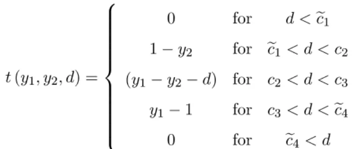
where t(y1; y2; d) = 8 > > > > > > > > > < > > > > > > > > > : 0 for d <ec1 1 y2 for ec1 < d < c2 (y1 y2 d) for c2 < d < c3 y1 1 for c3 < d <ec4 0 for ec4 < d
where ec1 = y2, c2 = maxfy1 1; y2g, c3 = minf1 y2; y1g and ce4 = y1. Note that c2 and c3 are de…ned as before, butec1 and ec4 di¤er fromc1 and c4.
Let T(y1; y2; d) = 8 > > > > > > > > > < > > > > > > > > > : 2 (1 y2)ec1+ 2 (1 y2)c2+ (y1 y2 c2)2 for d <ec1 2 (1 y2)d+ 2 (1 y2)c2+ (y1 y2 c2)2 for ec1 < d < c2 (y1 y2 d)2 for c2 < d < c3 2 (y1 1)d+ 2 (y1 1)c3+ (y1 y2 c3)2 for c3 < d <ec4 2 (y1 1)ec4+ 2 (y1 1)c3+ (y1 y2 c3)2 for ec4 < d We then de…ne the estimator of by minimizing
X
i
X
t<s
witsT yit; yis;(xit xis)0b
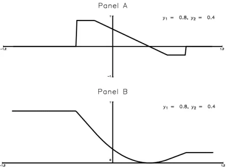
The function T and its derivative are depicted in Figures 8 and 9 for a pair of uncensored observations and for a pair with one censored and one uncensored observation, respectively.
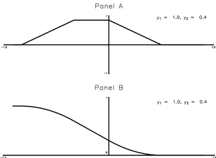
Figure 10 shows the moment condition and the expected value of the objective function when y1 N(0:5;1) and y2 N(0:4;1) and both are truncated from below at 0 and censored from above at 1.
As before, we also have
E t yit; yis(xit xis)0 (xit xis) = 0
where is convex and symmetric, and ( ) = 0( ) (when it exists) Let T (y1; y2; d) = 8 > > > > > > > > > < > > > > > > > > > : (1 y2)ec1+ (1 y2)c2+ (y1 y2 c2) for d <ec1 (1 y2)d+ (1 y2)c2+ (y1 y2 c2) for ec1 < d < c2 (y1 y2 d) for c2 < d < c3 (y1 1)d+ (y1 1)c3+ (y1 y2 c3) for c3 < d <ec4 (y1 1)ec4+ (y1 1)c3+ (y1 y2 c3) for ec4 < d
Figure 8: The Functionst(y1; y2; ) and T(y1; y2; ). Neither Observation Censored.
Figure 10: The FunctionsE[t(y1; y2; )]and E[T(y1; y2; )].
We then de…ne the estimator of by minimizing
X
i
X
t<s
witsT yit; yis;(xit xis)0b :
4.2 Pairwise Di¤erence Versions
If we can estimate a panel data with 2 observations per unit, then we can apply the same idea to any two observations in a cross section, treating the constant in the cross sectional model as an individual–speci…c e¤ect. This idea was explicitly used in Honoré and Powell (1994) to construct estimators for the parameters of cross sectional (one–sided) censored and truncated regression mod-els based on the panel data estimator in Honoré (1992). Among others, this also characterizes the relationship between the estimators in Manski (1987) and Han (1987) and between the estimators in Kyriazidou (1997) and Powell (1987). The same idea can be applied to the models with two–sided censoring and truncation considered here, and the asymptotic properties follow from the arguments used in Honoré and Powell (1994):
4.3 General Censoring Points.
It is easy to generalize the results above to the case where the truncation and censoring points are not all 0and 1. For example, consider the model with two–sided censoring
yit= 8 > > > < > > > : Li if yit< Li x0it +"it if Li yit Ui Ui if yit> Ui then yit Li Ui Li = 8 > > > < > > > : 0 if yit< Li xit Ui Li 0 +"it Li Ui Li if Li yit Ui 1 if yit> Ui
and we could estimate by
b= arg min b X i X t<s witsU yit Li Ui Li ;yis Li Ui Li ; xit xis Ui Li 0 b (19)
This simple approach does not work when the censoring points are time–varying, because then
"it Lit
Uit Lit is not stationary.
In order to proceed, we need explicit expressions for the di¤erence in these “re–censored”residu-als. We …rst note that only pairs for which the support of the re–censored residuals overlap can play a role in the moment conditions leading to the objective function. These pairs are characterized by
Lit Uis < x0it x0is < Uit Lis
and for such pairs, the di¤erence in the arti…cially censored residuals for individual i in periodst and sis
mami Lis x0is ; yit x0it ; Uis x0is mami Lit x0it ; yis x0is ; Uit x0it
= mami Lis; yit x0it x0is ; Uis mami Lit; yis+ x0it x0is ; Uit + x0it x0is
where we use the notationmamifa; x; bg= maxfa;minfx; bgg. If we de…ne k(L; U; y; d) = 8 > > > < > > > : U for d < y U y d y U < d < y L L for d > y L and
then
E u yit; yis; x0it x0is ; Lit; Lis; Uit; Uis (xit; xis) = 0
and hence
E u yit; yis; x0it x0is ; Lit; Lis; Uit; Uis (xit xis) = 0:
These will be the moment conditions that lead to the estimator in this case. Also de…ne K(L; U; y; d) = 8 > > > < > > > : 2yU 2dU U2 for d < y U (y d)2 y U < d < y L 2yL 2dL L2 for d > y L S(y1; y2; d; L1; L2; U1; U2) =K(L2; U2; y1; d) +K(L1; U1; y2; d) d2 and V (y1; y2; d; L1; L2; U1; U2) = 8 > > > < > > > : S(y1; y2; L1 U2; L1; L2; U1; U2) for d < L1 U2 S(y1; y2; d; L1; L2; U1; U2) for L1 U2< d < U1 L2 S(y1; y2; U1 L2; L1; L2; U1; U2) for d > U1 L2
and the estimator for is then de…ned by
arg min b n X i=1 X t<s witsV yit; yis;(xit xis)0b; Lit; Lis; Uit; Uis
A version of this can be developed for a general loss function.
All of these extensions assume that the censoring and truncation points are exogenous in the sense that one must make assumptions on the error terms conditional on them. In a recent paper, Khan, Ponomareva, and Tamer (2011) consider a (one–sided) censored regression model with en-dogenous censoring. Their approach only leads to partial identi…cation, but it would be interesting to generalize it to more general versions of the models considered here.
5
Empirical Application
In this section we apply the estimator in Section 2.1 to analyze the portfolio-reshu- ing e¤ect of a tax reform that increased the after-tax capital income on bonds relative to stocks in Denmark in 1987. We use a panel data set constructed from administrative records covering two years before and after the reform to estimate a portfolio share equation for bonds as a function of marginal tax
rates on capital income. The analysis presented here follows the literature on taxation and portfolio structure, e.g., Feldstein (1976), Hubbard (1985), King and Leape (1998), Samwick (2000), Poterba and Samwick (2002), Poterba (2002) and Alan, Crossley, Atalay, and Jeon (2010). These papers analyze (repeated) cross sections of households.6 Here the analysis is extended by using panel data and controlling for time–invariant correlated heterogeneity, i.e., …xed e¤ects. Controlling for correlated unobserved …xed factors is likely to be important in this context, since the portfolio composition of a household is likely to be in‡uenced by time–invariant factors such as risk aversion and time discounting.
In the next subsection we give a brief overview over the tax reform. After this, we introduce the data and present the results.
5.1 The Tax Reform
The tax reform, announced in 1985 and implemented in 1987, broke the link between the marginal tax rates on earned income and capital income. Before the reform, all income was taxed at the same marginal tax rate. With the reform the tax rate on positive capital income for high-income households was decreased from 73 percent to 56 percent. The reform thereby increased the after-tax return on interest-bearing assets and therefore encouraged households to shift their portfolios toward such assets. The reform also changed the tax value of interest deductions from 73 to about 50 percent, and this substantially increased the cost of debt, primarily mortgages, for leveraged high-income households. For such households the reform e¤ectively brought a negative wealth shock, giving them a strong incentive to lower their debt burden.7
The exact changes, however, di¤ered across municipalities. The Danish income tax system is built around a proportional local government tax and a progressive tax collected by the central government. While the progressive schedule is the same for everybody in Denmark, the local
6Bakija (2000) uses the limited panel module of the American Survey of Consumer Finances (SCF) to study
portfolio changes around the 1988 tax reform. However, his data set is very small (984 households) and unrepre-sentative due to the well-known attrition problem in the SCF panel module; see Kennickell and Woodburn (1997). More important in this context, the estimators applied do not exploit the full potential of the panel data in handling unobserved heterogeneity. Ioannides (1992) also employs the 1983-1986 SCF panel module but does not control for unobserved heterogeneity.
7Alan and Leth-Petersen (2006) document that the reduced value of the interest deduction led households to
liquidate …nancial assets to lower their mortgage debt. This was possible because pre-payment of mortgage debt is not restricted in Denmark.
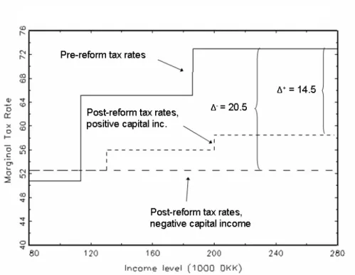
Figure 11: Marginal Tax Rate for High–Tax Municipality.
government tax rates vary across municipalities. A tax ceiling, however, insured that the marginal tax rate could be at the maximum 73 percent. After the reform the tax ceiling on earned income was reduced to 68 percent in the highest bracket8 and 56 percent in the middle bracket. Capital income was now taxed at the same rate independently of the level of earned income. The marginal tax rates across tax brackets before and after the reform are summarized in Table 1 (see Appendix 2)
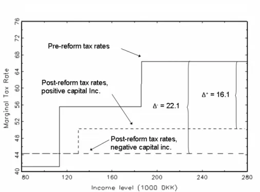
The application of a tax ceiling together with the heterogeneous local government tax rates implies that the reform had di¤erential e¤ects on people living in di¤erent municipalities. Figures 11 and 12 illustrate the changes in marginal tax rates due to the reform for a high-tax and a low-tax municipality, respectively.
For a high-income person living in the municipality with the high local government tax, the marginal tax rate on positive net capital income falls by 14.5 percentage points and the marginal tax rate on negative net capital income falls by 20.5 percentage points. For a similar person living in the municipality with the low local government tax rate, the marginal tax rate on positive
Figure 12: Marginal Tax Rate for Low–Tax Municipality.
net capital income falls by 16.1 percentage points and negative net capital income falls by 22.1 percentage points. It is these di¤erences in changes of marginal tax rates that we will exploit for identifying the e¤ect of changes in marginal tax rates on the portfolio allocation when using the …xed e¤ects estimator.
The marginal tax rates on capital income refer to income received in the form of dividends on stocks and interest payments from interest bearing accounts and bonds. Both before and after the reform, realized capital gains/losses associated with trading assets were generally not taxed. The exemption from this rule is capital gains from corporate stocks held for less than three years. Such capital gains are taxed as earnings. Dividend payments were low relative to interest received from bonds.9 This suggests that lowering the marginal tax rate on positive capital income a¤ected bonds and stocks di¤erentially, favoring mainly income from bonds. In the empirical analysis we therefore focus on reshu- ing between bonds and stocks.
9
The median household in the sample holding stocks received dividends corresponding to 2 percent of the value of the stocks. The median household in the sample holding bonds received interest payments from these corresponding to 10 percent of the value of the bonds.
5.2 Data
The data set is drawn from a random sample of 10 percent of the Danish population observed in the years 1984 to 1988. Information on portfolio allocations, income, wealth and demographics is collected and merged from di¤erent public administrative registers for all adult members of the household that the sampled person belongs to. Portfolio and income information is obtained from the income tax register. The portfolio information exists because Denmark had a wealth tax that required all wealth holdings to be reported to the tax authorities. This information allows us to break the wealth of each household into holdings of stocks and bonds. “Stocks” includes all holdings of publicly and privately traded stocks, and “bonds” includes government and corporate bonds. The holdings of stocks and bonds are self–reported through the tax return and then audited by the tax authority.
5.2.1 Sample selection
For our analysis we exclude observations if one of the household members is self-employed, since register data are not likely to contain a good measure of own business wealth and because taxable income is quite volatile for those individuals. Sampled individuals younger than 18 or older than 60 are dropped as are students and individuals living together with his/her parents or living in a common household, i.e., a household with more than one family. To keep the focus on the importance of tax incentives, we include only stable couples, i.e., couples where the partner is the same in 1984 through 1988. On the same grounds we also exclude couples moving in the sample period. For the purpose of the analysis we require that households entering the sample be observed in all years in the period 1984-1988 so that we have a balanced panel.
Our objective is to investigate whether households reshu- e their portfolios in response to a change in tax incentives. As in most industrialized countries many Danish households have fairly undiversi…ed portfolios. Since the decrease in the value of interest deductions generated a large negative wealth shock, clearly, these households are not likely to engage in portfolio reshu- ing and hence cannot give us a clean answer regarding portfolio readjustments. We therefore construct a sub-sample of households holding positive amounts of stocks or bonds of at least 5,000 DKK in 1984. We also require households to hold a positive amount of either stocks or bonds throughout the rest of the observation period. This selection is introduced because we want to focus on households with a potential to reshu- e between stocks and bonds. Also renters are deselected because there
are few renters with diversi…ed portfolios.10 The …nal subsample includes 8,577 households.11
5.3 Results
In this section we investigate if households reshu- ed their portfolio of bonds and stocks as a response to the changes in relative after-tax returns on assets brought about by the 1987 tax reform. To do, this we employ the estimator presented above and estimate a portfolio share equation where the fraction of bonds in …nancial wealth, de…ned as the sum of bonds and stocks, is regressed on the marginal tax rate on positive capital income and some control variables.
The distinguishing feature of our data set is the panel dimension. This facilitates estimating portfolio share equations allowing for correlated unobserved time–invariant heterogeneity. This is important because we believe that unobserved time–invariant factors, such as risk aversion and time preferences, are correlated with wealth. High risk aversion may, for example, lead to a higher portfolio share of safe assets, such as bonds, for a given level of wealth.
Before the reform, capital income and earnings were lumped together and taxed according to a progressive tax scheme. This implies that households choose their tax bracket when choosing their portfolios and that the marginal tax rate on capital income is likely to be an endogenous regressor. We address this by calculating the marginal tax rate on capital income based on the household’s income in 1984, the year before the reform was announced, but using current year rules. In this way the individual level tax bracket is allocated based on information that was predetermined relative to the portfolio response to the reform.
We regress portfolio shares on the marginal tax rate on positive capital income, the log of total …nancial assets, i.e., assets held in stocks and bonds, and a set of year dummies. Tax rate changes vary across municipalities, but most of the change in tax rates is common across municipalities. Year dummies control for the e¤ect of this common part, thereby also removing the major part of the wealth e¤ect brought about by the reform. E¤ectively, by introducing year dummies, the coe¢ cients on marginal tax rates are identi…ed by di¤erences in changes of marginal tax rates. Year dummies may also pick up common e¤ects related to ‡uctuations in assets. Financial assets
1 0For assessing portfolio reshu- ing renters could have been included. We have chosen to leave them out of this
analysis because there are only a few renters (898) with positive …nancial wealth of at least 5000 DKK in 1984. Moreover, renters generally do not provide a good comparison group for homeowners, since di¤erent preference parameters may govern their behavior.
1 1
control for any remaining wealth e¤ect that might be present.12
Table 2 of Appendix 2 presents the parameter estimates from estimating random e¤ects Tobit and …xed e¤ects censored regression models for the portfolio share of bonds in …nancial wealth. The estimated parameter on the marginal tax rate is negative.13 If year dummies and …nancial assets pick up the wealth e¤ect related to the reform, in particular the e¤ect of the reduction in the value of interest deduction that led households to liquidate …nancial assets, then this is exactly what economic theory predicts. Households should substitute from stocks toward bonds, whose relative after-tax return increased, and this is what the results indicate.
Considering the corresponding random e¤ects estimates, we can see that the parameter esti-mates on …nancial assets and on year dummies are quite di¤erent, and the test of equality of all the parameters in the random e¤ects and …xed e¤ects speci…cations rejects.
6
Concluding Remarks
This paper constructs estimators for panel data regression models with individual speci…c hetero-geneity and two–sided censoring and truncation. Following Powell (1986) the estimation strategy is based on moment conditions constructed from re–censored or re–truncated residuals. While these moment conditions do not identify the parameter of interest, they can be used to motivate objective functions that do. This part is the main methodological contribution of the paper. We apply one of the estimators to study the e¤ect of a Danish tax reform on household portfolio choice. We …nd that a random e¤ects speci…cation can be rejected in favor of the “…xed”e¤ects speci…cation stud-ied here, although both models yield the same sign of the key parameter that one would anticipate from economic theory. The estimators are fairly easy to implement and a link to a program that calculates the leading estimator is provided at http://www.princeton.edu/~honore/stata.
1 2
An alternative identi…cation strategy could be based on comparing the behavior of households in di¤erent tax brackets. Households in the lowest tax bracket faced only very small changes in marginal tax rates on capital income, and households in the middle tax bracket faced di¤erent changes in marginal tax rates than households in the highest tax bracket. In our case this is not a natural approach to follow. High–and low–income people are di¤erent in terms of wealth levels and portfolio composition and possibly di¤erent with respect to preference parameters such as the discount rate and the level of risk aversion. Households in lower tax brackets therefore do not represent a natural control group for high–income households.
1 3
As explained in Honoré (2008), the parameter estimates for both the random e¤ects and the …xed e¤ects models can be converted to marginal e¤ects by multiplying them by the fraction of observations that are not censored.
References
Abrevaya, J. (1999): “Rank estimation of a transformation model with observed truncation,”
Econometrics Journal, 2(2), 292–305.
Alan, S., T. Crossley, K. Atalay, and S.-H. Jeon (2010): “New Evidence on Taxes and Portfolio Choice,”Journal of Public Economics, 94, 813–823.
Alan, S., and S. Leth-Petersen (2006): “Tax Incentives and Household Portfolios: A Panel Data Analysis,” Center for Applied Microeconometrics, University of Copenhagen, Working pa-per number 2006-13.
Amemiya, T.(1985): Advanced Econometrics. Harvard University Press.
Andrews, M., T. Schank,andR. Simmons(2005): “Does Worksharing Work? Some Empirical Evidence from the IAB-Establishment Panel,”Scottish Journal of Political Economy, 52(2).
Arellano, M., and B. E. Honoré (2001): “Panel Data Models. Some Recent Developments,”
Handbook of Econometrics, 5, Elsevier Science, Amsterdam.
Bakija, J.(2000): “The E¤ect of Taxes on Portfolio Choice: Evidence from Panel Data Spanning the Tax Reform Act of 1986,” Williams College.
Charness, G., G. Frechette, and J. Kagel (2004): “How Robust Is Laboratory Gift Ex-change?,”Experimental Economics, 7(2), 189–205.
Chen, S. (forthcoming): “Nonparametric Identi…cation and Estimation of Truncated Regression Models,”Review of Economic Studies.
de Figueriredo, J., and E. Tiller (2001): “The Structure and Conduct of Corporate Lobby-ing: How Firms Lobby the Federal Communications Commission,”Journal of Economics and
Management Strategy, 10(1), 91–122.
Fehr, E., E. Kirchler, A. Weichbold, and S. Gachter(1998): “When Social Norms Over-power Competition: Gift Exchange in Experimental Labor Markets,”Journal of Labor
Eco-nomics, 16(2), 324–351.
Feldstein, M.(1976): “Personal Taxation and Portfolio Composition: An Econometric Analysis,”
Fenn, G., and N. Liang (2001): “Corporate Payout Policy and Managerial Stock Incentives,”
Journal of Financial Economics, 60(1), 45–72.
Ferrie, J. P., and K. Rolf (2011): “Socioeconomic Status in Childhood and Health after Age 70: A New Longitudinal Analysis for the U.S., 1895-2005,”SSRN eLibrary.
Gifford, K., and J. Bernard (2005): “In‡uencing Consumer Purchase Likelihood of Organic Food,”International Journal of Consumer Studies, pp. 1–9.
Han, A. (1987): “Nonparametric Analysis of a Generalized Regression Model: The Maximum Rank Correlation Estimator,”Journal of Econometrics, 15.
Honoré, B. E.(1992): “Trimmed LAD and Least Squares Estimation of Truncated and Censored Regression Models with Fixed E¤ects,”Econometrica, 60, 533–565.
(2008): “On Marginal E¤ects in Semiparametric Censored Regression Models,”Princeton University.
Honoré, B. E., and L. Hu (2004): “Estimation of Cross Sectional and Panel Data Censored Regression Models with Endogeneity,”Journal of Econometrics, 122(2), 293–316.
Honoré, B. E., and J. L. Powell (1994): “Pairwise Di¤erence Estimators of Censored and Truncated Regression Models,”Journal of Econometrics, 64, 241–78.
Honoré, B. E., and J. L. Powell (1994): “Pairwise Di¤erence Estimators of Censored and Truncated Regression Models,”Journal of Econometrics, 64(1-2), 241–78.
Houston, J., andM. Ryngaert(1997): “Equity Issuance and Adverse Selection: A Direct Test Using Conditional Stock O¤ers,”Journal of Finance, 52(1), 197–219.
Hu, L.(2002): “Estimation of a Censored Dynamic Panel Data Model,”Econometrica, 70(6), pp. 2499–2517.
Huang, M.,andR. Hauser(1998): “Trends in Black-White Test Score Di¤erences: WORDSUM Vocabulary Test,” in The Rising Curve: Long-IQ and Related Measures, ed. by U. Neisser, pp. 303–332. American Psychological Association, Washington, D.C.
(2001): “Convergent Trends in Black-White Verbal Test Score Di¤erentials in the U.S.: Period and Cohort Perspectives,”EurAmerica, 31(2), 185–230.
Hubbard, R. G. (1985): “Personal Taxation, Pension Wealth, and Portfolio Composition,”The
Review of Economics and Statistics, 67(1), 53–60.
Ioannides, Y. (1992): “Dynamics of the Composition of Household Asset Portfolios and Life Cycle,”Applied Financial Economics, 2(3), 145–159.
Kennickell, A., and L. Woodburn (1997): “Weighting Design for the 1983-89 SCF Panel,” Washington DC: Federal Reserve Board of Governors.
Khan, S., M. Ponomareva, and E. Tamer(2011): “Identi…cation of Panel Data Models with Endogenous Censoring,” MPRA Paper 30373, University Library of Munich, Germany.
King, M., and J. Leape (1998): “Wealth and Portfolio Composition: Theory and Evidence,”
Journal of Public Economics, 69(2), 155–193.
Kyriazidou, E.(1997): “Estimation of a Panel Data Sample Selection Model,”Econometrica, 65, 1335–1364.
Lafontaine, F. (1993): “Contractual Arrangements as Signalling Devices: Evidence from Fran-chising,”Journal of Law, Economics, and Organization, 9(2), 256–289.
Manski, C. (1987): “Semiparametric Analysis of Random E¤ects Linear Models from Binary Panel Data,”Econometrica, 55, 357–62.
McMillan, J., and C. Woodruff (1999): “Inter…rm Relationships and Informal Credit in Vietnam,”Quarterly Journal of Economics, 114(4), 1285–1320.
Nickerson, J., and B. Silverman (2003): “Why Aren’t All Truck Drivers Owner-Operators? Asset Ownership and the Employment Relation in Interstate For-Hire Trucking,”Journal of
Economics and Management Strategy, 12(1), 91–118.
Officer, M.(2004): “Collars and Renegotiation in Mergers and Acquisitions,”Journal of Finance, 59(6), 2719–2743.
Pakes, A., and D. Pollard(1989): “Simulation and the Asymptotics of Optimization Estima-tors,”Econometrica, 57, 1027–1057.
Petersen, M., and R. Rajan (1994): “The Bene…ts of Lending Relationships: Evidence from Small Business Data,”Journal of Finance, 49(1), 3–37.
(1995): “The E¤ect of Credit Market Competition on Lending Relationships,”Quarterly
Journal of Economics, 110(2), 407–443.
Poterba, J., and A. Samwick (2002): “Taxation and Household Portfolio Composition: US Evidence from the 1980s and 1990s,”Journal of Public Economics, 87(1), 5–38.
Poterba, J. M.(2002): “Taxation and Portfolio Structure: Issues and Implications,”inHousehold
Portfolios, ed. by L. Guiso, M. Haliassos,and T. Jappelli. MIT Press.
Powell, J. L. (1986): “Symmetrically Trimmed Least Squares Estimation for Tobit Models,”
Econometrica, 54(6), 1435–60.
(1987): “Semiparametric Estimation of Bivariate Latent Models,” Working Paper no. 8704, Social Systems Research Institute, University of Wisconsin–Madison.
Samwick, A.(2000): “Portfolio Responses to Taxation: Evidence from the End of the Rainbow,”
inDoes Atlas Shrug? The Economic Consequences of Taxing the Rich, ed. by J. Slemrod. Harvard
7
Appendix 1: Proofs and Derivations
7.1 Two–Sided Censoring
This section provides justi…cation for the statements about the estimators for the model with two– sided censoring. We …rst verify that u(yit; yis; x0it x0is ) in equation (8) does indeed yield the
di¤erence in the re-censored residuals de…ned in (6) and (7). Write d=x0it x0is , and consider …rst the case where d >0. In this case, the di¤erence in the re-censored residuals is
maxfyit d;0g minfyis;1 dg
which is most easily analyzed by considering a number of cases fordbetween0and 1. As mentioned earlier, the contribution to the moment condition should be 0 whendis outside the interval between
1and 1,which is consistent with the de…nition of u:
There are four cases based on combinations of whetheryit d 0and yis 1 d:14
Case 1 (yit d 0 and yis 1 d): In this case, maxfyit d;0g minfyis;1 dg =
(yit d) (1 d) =yit 1.
Case 2 (yit d 0 and yis 1 d): In this case, maxfyit d;0g minfyis;1 dg =
0 (1 d) =d 1.
Case 3 (yit d 0 and yis 1 d): In this case, maxfyit d;0g minfyis;1 dg =
(yit d) yis=yit yis d.
Case 4 (yit d 0andyis 1 d): In this case,maxfyit d;0g minfyis;1 dg= 0 yis=
yis.
Case 3 corresponds to values of d close to (or at) 0. Speci…cally, the region for Case 3 is
(0;minfyit;1 yisg) = (0; c3). Noting thatc2 0, it is clear thatmaxfyit d;0g minfyis;1 dg=
yit yis dis consistent with the de…nition ofu in equation (8).
Case 2 corresponds to values ofdclose to (or at ) 1, speci…cally the region(maxfyit;1 yisg;1) =
(c4;1), and it is again clear that u deliversmaxfyit d;0g minfyis;1 dg.
The region that de…nes the other two cases is (minfyit;1 yisg;maxfyit;1 yisg) = (c3; c4).
Cases 1 and 4 give di¤erent expressions depending on whether yit or 1 yis is larger, but these 1 4Since both the di¤erence in the re-censored residuals anduare continuous ind, it is not necessary to distinguish
expressions correspond exactly to the two cases for the max in the de…nition of u in (8) over the interval(c3; c4).
The case d <0 is dealt with in exactly the same manner. We now turn to the question of why
E U yit; yis;(xit xis)0b
is uniquely minimized at the true . This is the key for consistency of the proposed estimator. The result follows from the following lemma
Lemma 3 Suppose
yi1 = mamif0; +"i1;1g
and
yi2 = mamif0; "i2;1g
where "i1and "i2are identically distributed random variables with support on the whole real line.
Then arg max d2[ 1;1]E[U(yi1; yi2; d)] = 8 > > > < > > > : 1 if 1 if 1< <1 1 if 1 Proof: For1 d 0 E[u(yi1; yi2; d)] = E[maxfyi1 d;0g minfyi2;1 dg]
= E[maxfmamif0; +"i1;1g d;0g minfmamif0; "i2;1g;1 dg]
= E[maxfmamif0 d; d+"i1;1 dg;0g mamif0; "i2;1 dg]
= E[mamif0; d+"i1;1 dg mamif0; "i2;1 dg]
If"i1(and"i2) have full support, then this is negative for d > and positive ford < . For 1 d 0
E[u(yi1; yi2; d)] = E[minfyi1;1 +dg maxfyi2+d;0g]
= E[minfmamif0; +"i1;1g;1 +dg maxfmamif0; "i2;1g+d;0g]
= E[mamif0; +"i1;1 +dg maxfmamifd; "i2+d;1 +dg;0g]
If"i1(and"i2) have full support, then this is negative for d > and positive ford < . Since
E U0(yi1; yi2; d) =E[u(yi1; yi2; d)] the argument above shows that
arg max d2[ 1;1]E[U(yi1; yi2; d)] = 8 > > > < > > > : 1 if 1 if 1< <1 1 if 1
Corollary 4 Consider the model
yit = x0it +"it yit = 8 > > > < > > > : 0 if yit<0 yit if 0 yit 1 1 if yit>1
for t = 1;2. If "itis stationary conditional on (xi1; xi2) with support on the whole real line, then
the set of solutions to
max
b E U yi1; yi2;mami 1;(xi1 xi2)
0b;1
is
b:P mami 1;(xi1 xi2)0b;1 = mami 1;(xi1 xi2)0 ;1 = 1
The Corollary above requires that the errors are stationary conditional on the regressors. This is much more general than the usual assumption that the individual— speci…c e¤ect and the contem-poraneous errors interact additively. To see that E U yit; yis;(xit xis)0b in (12) is uniquely
minimized, it is convenient to assume that "it and "is are independent and identically
distrib-uted conditional on some individual— speci…c e¤ect, vi. With this assumption, the argument for
whyE U yit; yis;(xit xis)0b is uniquely minimized follows essentially the same logic as above.
Speci…cally, when1 d 0
(u(yit; yis; d)) = (mamif0; d+"it;1 dg mamif0; "is;1 dg)
If "itand "is are independent and identically distributed conditional on vi, then
E[ (u(yit; yis; ))jxit; xis] =E[E[ (u(yit; yis; ))j i; xit; xis]jxit; xis]
=E[E[ (mamif0; "it;1 g mamif0; "is;1 g)j i; xit; xis]jxit; xis] = 0
because mamif0; "it;1 g mamif0; "is;1 g is symmetrically distributed conditional on i,
and ( ) is an odd function. For d >
mamif0; d+"it;1 dg mamif0; "is;1 dg
mamif0; "it;1 dg mamif0; "is;1 dg
with probability 1 (conditional on i), and since is increasing
E[ (mamif0; d+"it;1 dg mamif0; "is;1 dg)j i; xit; xis]
E[ (mamif0; "it;1 dg mamif0; "is;1 dg)j i; xit; xis] = 0
The line of argument is the same when d < . Strict inequalities follow from a full support assumption on"i1(and"i2).
We therefore have that E[U (yit; yis; d)jxit; xis] is decreasing to the left of (xit xis)0 and
increasing to the right. Hence it is minimized at d = (xit xis)0 . Subject to a rank condition,
this implies that E U yit; yis;(xit xis)0b xit; xis is minimized atb= :
7.2 Two–Sided Truncation
The following Lemma (combined with the obvious rank–condition) establishes that minimization of E R yi1; yi2;(xi1 x2i)0b will identify if the distribution of "is log–concave. This is the
assumption that was made in a number of other papers (including Honoré (1992), Honoré and Powell (1994) and Abrevaya (1999); see also the discussion in Chen (forthcoming)). In Section 2.2, we only consider the case with (two–sided) truncation at 0 and 1. It is just as easy to prove identi…cation for general individual– and time–speci…c truncation points. In the following we therefore denote the truncation points by Land U.
Lemma 5 Let (L; U) be a vector of random variables such thatL < U with probability 1. Assume
that "is independent of (L; U) and has a continuous, log–concave distribution with support on the
(yi2; Li2; Ui2) from the distribution of (y; L; U) conditional on L < y < U. then E[R (yi1; yi2; d)]
is uniquely minimized at d= i1 i2.
7.3 Proof of Lemma 5.
LetE denote expectation conditional on truncation and E in population. The moment condition can then be written as
E[ (4yi 4di) 1fLi2 di2 yi1 di1 Ui2 di2g1fLi1 di1 yi2 di2 Ui1 di1g] = E[ (4yi 4di) 1fLi2+4di yi1 Ui2+4dig1fLi1 4di yi2 Ui1 4dig] = E[ (4"i+4 i 4di) 1fLi2 (4 i 4di) "i1+ i2 Ui2 (4 i 4di)g 1fLi1+ (4 i 4di) "i2+ i1 Ui1+ (4 i 4di)g] where4ai=ai1 ai2. Letting i = (4 i 4di) = E[ (4"i+ i) 1fLi2 i2 i "i1 Ui2 i2 ig1fLi1 i1+ i "i2 Ui1 i1+ ig] = E [ (4"i+ i) 1fLi2 i2 i "i1 Ui2 i2 ig1fLi1 i1+ i "i2 Ui1 i1+ ig 1fLi1 yi1 Ui1g1fLi2 yi2 Ui2g] 1 P(Li1 yi1 Ui1; Li2 yi2 Ui2) :
It su¢ ces to show that this is nonpositive for i<0, strictly negative in a neighborhood to the
left of 0, 0 for i = 0; nonnegative for i >0, and strictly positive in a neighborhood to the right
of 0. Now consider the term
E [ (4"i+ i) 1fLi2 i2 i "i1 bj i2 ig1fLi1 i1+ i "i2 Ui1 i1+ ig
1fLi1 i1 "i1 Ui1 i1g1fLi2 i2 "i2 bj i2g]:
De…ning wi1 = 12("i1 "i2) and wi2 = 12("i1+"i2) (so "i1 = (wi1+wi2) and "i2 =wi2 wi1 and 4"i = 2wi1)
E [ (4"i+ i) 1fLi2 i2 i "i1 Ui2 i2 ig1fLi1 i1+ i "i2 Ui1 i1+ ig 1fLi1 i1 "i1 Ui1 i1g1fLi2 i2 "i2 Ui2 i2g] = E [ (2wi1+ i) 1fLi2 i2 i wi1+wi2 Ui2 i2 ig 1fLi1 i1+ i wi2 wi1 Ui1 i1+ ig 1fLi1 i1 wi1+wi2 Ui1 i1g 1fLi2 i2 wi2 wi1 Ui2 i2g] = E [ (2wi1+ i) 1 Li2 i2 wi2 1 2 i wi1+ 1 2 i Ui2 i2 wi2 1 2 i 1 Ui1+ i1+wi2 1 2 i wi1+ 1 2 i Li1+ i1+wi2 1 2 i 1 Li1 i1 wi2+ 1 2 i wi1+ 1 2 i Ui1 i1 wi2+ 1 2 i 1 Ui2+ i2+wi2+ 1 2 i wi1+ 1 2 i Li2+ i2+wi2+ 1 2 i ] = E [ (2wi1+ i) 1fmax Li2 i2 wi2 1 2 i; Ui1+ i1+wi2 1 2 i; Li1 i1 wi2+ 1 2 i; Ui2+ i2+wi2+ 1 2 i wi1+ 1 2 i min Ui2 i2 wi2 1 2 i; Li1+ i1+wi2 1 2 i; Ui1 i1 wi2+ 1 2 i; Li2+ i2+wi2+ 1 2 i g] = E (2wi1+ i) 1 ci wi1+ 1 2 i ci = E E (2wi1+ i) 1 ci wi1+ 1 2 i ci wi2; Li1; Ui1; Li2; Ui2 whereci= min Ui2 i2 wi2 12 i; Li1+ i1+wi2 12 i; Ui1 i1 wi2+12 i; Li2+ i2+wi2+ 12 i .
It therefore follows that E E (2wi1+ i) 1 ci wi1+ 1 2 i ci wi2; Li1; Ui1; Li2; Ui2 8 > > > > > > > > > < > > > > > > > > > : 0 if i <0 <0 if i <0, P ci wi1+12 i ci >0 = 0 if i = 0 0 if i >0 >0 if i >0, P ci wi1+12 i ci >0:
Since the "’s (and hence the wi’s) are continuous, the condition thatP ci wi1+12 i ci >0
will be satis…ed ifP(ci >0)>0.
We will next show that for i2(0; k),P(ci >0)>0 for somek >0. Note that
1fci >0g = 1 Li1+ i1+wi2 1 2 i >0 1 Ui1 i1 wi2+ 1 2 i>0 1 Li2+ i2+wi2+ 1 2 i>0 1 Ui2 i2 wi2 1 2 i>0 = 1 wi2 > Li1 i1+ 1 2 i 1 Ui1 i1+ 1 2 i> wi2 1 wi2> Li2 i2 1 2 i 1 Ui2 i2 1 2 i> wi2 = 1 Ui1 i1+ 1 2 i > wi2 > Li1 i1+ 1 2 i 1 Ui2 i2 1 2 i> wi2> Li2 i2 1 2 i :
This will have positive probability provided that
P Li1 i1+
1
2 i < Ui2 i2 1
2 >0
which follows from Lemma 6.
Lemma 6 If (U1; V1) and (U2; V2) are two independent draws of a random vector (U; V) with
P(U < V) = 1, then there exists a k >0 such that for 0< < k, P(U1 < V2 )>0.
Proof. Since V U > 0 with probability 1, there exists anm > 0 such that P(V U > m)
1
2. Now consider the space f(u; v) :v u > mg. This can be divided into a countable number of regions, Ak, such that for (u1; v1);(u2; v2) 2 Ak, ju1 u2j < m2 and jv1 v2j < m2. Since
P(V U > m) = 12, at least one of these regions, Ak, must have positive probability. Hence there
is positive probability that(U1; V1)and (U2; V2) in the statement of the lemma both belong to this
8
Appendix 2: Empirical Results
Table 1: Marginal tax rates before and after implementation of the 1987 tax reform
Before Reform After Reform
Tax bracket Earnings + Cap inc Tax bracket Earnings inc<0 inc: >0(1) 0-113 M + 19:75 0 130 M+ 22:00 M+ 22:00 M+ 22:00
113-186 M + 34:15 130 200 M+ 28:00 M+ 22:00 M+ 28:00
186- M + 44:95 200 M+ 40:00 M+ 22:00 M+ 28:00
Tax ceiling 73 Tax ceiling 68:00=56:00(2) 56:00
Note: M is the local government tax rate. Threshold values for the tax brackets are given in 1000 DKK. Thresholds are adjusted yearly. Threshold values used in the table are for 1986 (before the reform) and 1987 (after the reform). The marginal tax rates refer to personal income (as opposed to household income).
(1) The tax brackets for positive net capital income refer to the sum of earnings and positive net capital income.
After the reform positive capital income is taxed progressively up to the …rst threshold, 130,000 DKK. For a married couple the progression threshold is 260,000 based on the sum of their joint positive net capital income and earnings.
Table 2:. Random and Fixed E¤ects Censored Regression Estimates of the Portfolio Share of Bonds in Financial Wealth.
Fixed E¤ects Random E¤ects
MTR capital income 0:130 0:206 (0:071) (0:045) Ln(Financial Assets) 0:177 0:085 (0:008) (0:003) D85 0:214 0:157 (0:006) (0:006) D86 0:314 0:248 (0:009) (0:006) D87 0:318 0:285 (0:013) (0:008) D88 0:383 0:331 (0:013) (0:008) Constant — 0:047 (0:046) # households/observations 8,577 / 42,885 # left/right censored obs 7,529 / 15,655 Test of Parameter Equality (d.f.) 167 (6)
![Figure 5: The Functions E [u (y 1 ; y 2 ; )] and E [U (y 1 ; y 2 ; )]. where U (y 1 ; y 2 ; d) = 8>>>>>>>>>>>>>>>< > > > > > > > > > > > > > > > : 1 + 2c 1 + c 21](https://thumb-us.123doks.com/thumbv2/123dok_us/9487996.2824114/11.918.237.680.126.460/figure-functions-e-e-u-u-gt-gt.webp)
![Figure 7: The Functions E [r (y 1 ; y 2 ; )] and E [R (y 1 ; y 2 ; )].](https://thumb-us.123doks.com/thumbv2/123dok_us/9487996.2824114/14.918.236.686.643.978/figure-functions-e-r-y-y-e-r.webp)
![Figure 10: The Functions E [t (y 1 ; y 2 ; )] and E [T (y 1 ; y 2 ; )].](https://thumb-us.123doks.com/thumbv2/123dok_us/9487996.2824114/22.918.234.684.124.461/figure-functions-e-t-y-y-e-t.webp)