OPTIMAL MARTINGALE MEASURES AND HEDGING
IN MODELS DRIVEN BY L´
EVY PROCESSES
By
Jozef Kollar
Submitted for the Degree of Doctor of Philosophy at Heriot-Watt University on Completion of Research in the
School of Mathematical and Computer Sciences and the Maxwell Institute for Mathematical Sciences
July 2011.
This copy of the thesis has been supplied on the condition that anyone who consults it is understood to recognise that the copyright rests with its author and that no quo-tation from the thesis and no information derived from it may be published without the prior written consent of the author or the university (as may be appropriate).
I hereby declare that the work presented in this the-sis was carried out by myself at Heriot-Watt University, Edinburgh, except where due acknowledgement is made, and has not been submitted for any other degree.
Jozef Kollar (Candidate)
Dr Anke Wiese (Supervisor)
Dr Terence Chan (Supervisor)
Abstract
Our research falls into a broad area of pricing and hedging of contingent claims in incomplete markets. In the first part we introduce the L´evy processes as a suitable class of processes for financial modelling purposes. This in turn causes the mar-ket to become incomplete in general and therefore the martingale measure for the pricing/hedging purposes has to be chosen by introducing some subjective criteria. We study several such criteria in the second section for a general stochastic volatility model driven by L´evy process, leading to minimal martingale measure, variance-optimal, or the more general q-optimal martingale measure, for which we show the convergence to the minimal entropy martingale measure forq ↓1.
The martingale measures studied in the second section are put to use in the third section, where we consider various hedging problems in both martingale and semimartingale setting. We study locally risk-minimization hedging problem, mean-variance hedging and the more general p-optimal hedging, of which the mean-variance hedging is a special case for p = 2. Our model allows us to explicitly determine the variance-optimal martingale measure and the mean-variance hedg-ing strategy ushedg-ing the structural results of Gourieroux, Laurent and Pham (1998) extended to discontinuous case by Arai (2005a).
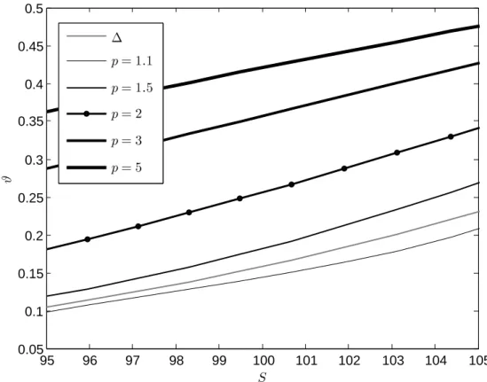
Assuming a Markovian framework and appealing to the Feynman-Kac theorem, the optimal hedge can be found by solving a three-dimensional partial integro-differential equation. We illustrate this in the last section by considering the variance-optimal hedge of the European put option, and find the solution numeri-cally by applying finite difference method.
Acknowledgements
First of all, I would like to thank my advisors Dr Anke Wiese and Dr Terence Chan for sharing their knowledge, their patience and support throughout my studies and work on this thesis. I am especially grateful to Dr Weise for her persistence in teaching me a good style of mathematics, for her editorial and technical comments, which improved this work in an essential way.
I would also like to thank my PhD buddy Chenming, Seva, Erik, Professor Foss and Professor Kyprianou for many interesting discussions and all their support.
My greatest thanks go to my family. I wish to thank my parents, my wife Ida and my daughters Terezia and Agnesa for their unconditional love. Thank you for being there for me!
ACADEMIC REGISTRY
Research Thesis Submission
Name:
School/PGI: Version: (i.e. First,
Resubmission, Final)
Degree Sought (Award and
Subject area)
Declaration
In accordance with the appropriate regulations I hereby submit my thesis and I declare that: 1) the thesis embodies the results of my own work and has been composed by myself
2) where appropriate, I have made acknowledgement of the work of others and have made reference to work carried out in collaboration with other persons
3) the thesis is the correct version of the thesis for submission and is the same version as any electronic versions submitted*.
4) my thesis for the award referred to, deposited in the Heriot-Watt University Library, should be made available for loan or photocopying and be available via the Institutional Repository, subject to such conditions as the Librarian may require
5) I understand that as a student of the University I am required to abide by the Regulations of the University and to conform to its discipline.
* Please note that it is the responsibility of the candidate to ensure that the correct version of the thesis is submitted.
Signature of Candidate:
Date:
Submission
Submitted By (name in capitals):
Signature of Individual Submitting:
Date Submitted:
For Completion in Academic Registry
Received in the Academic Registry by (name in capitals): Method of Submission
(Handed in to Academic Registry; posted through internal/external mail):
E-thesis Submitted (mandatory from November 2008)
Signature: Date:
Jozef Kollar
Final PhD
Financial Mathematics Mathematics and Computer Science
Contents
Abstract iii
Acknowledgements iv
1 Introduction 1
2 L´evy processes in Finance 4
2.1 Introduction . . . 4
2.2 Stochastic exponential and exponential martingale . . . 8
2.3 Models . . . 10
2.4 Absolutely continuous measure changes . . . 13
3 Optimal martingale measures 18 3.1 Introduction . . . 18
3.2 The minimal martingale measure . . . 19
3.3 The variance-optimal martingale measure . . . 21
3.3.1 Cern´ˇ y-Kallsen approach . . . 30
3.4 The minimal entropy martingale measure . . . 32
3.5 The q-optimal martingale measure . . . 37
3.5.1 Convergence to the minimal entropy martingale measure . . . 49
4 Optimal hedging 55 4.1 Introduction . . . 55
4.2 Local risk-minimization hedging . . . 57
4.2.1 Martingale setting . . . 58
4.3 Mean-variance hedging . . . 64
4.3.1 Semimartingale setting . . . 66
4.3.2 Equivalent variance-optimal martingale measure . . . 73
4.4 The p-optimal hedging . . . 77
5 Numerical results 85 5.1 Introduction . . . 85
5.2 Model specifications . . . 85
5.3 European put . . . 88
5.3.1 Change of variables . . . 88
5.3.2 Finite difference method . . . 90
5.3.3 Computation of hedge ratios . . . 91
5.4 Option on realized variance . . . 93
Chapter 1
Introduction
A Brownian motion is a stochastic process with independent, stationary increments of Gaussian distribution. It is without any doubt the most widely used process for the modelling of price fluctuations, whether considered in the Black-Scholes frame-work or more general diffusion models. The common property of these models is continuity, the property not observed in the price movement, as the prices move by jumps. However this is not the only reason for considering models with jumps. Many properties desirable from the models of price movement, either at the econometric or option pricing level, can only be obtained in diffusion models by considering very ex-treme parameters, while the same desirable properties can be easily obtained almost by definition when considering processes with jumps. L´evy processes represent one such class of processes. They share the common properties with Brownian motion that their increments are independent and stationary while having discontinuous paths in general. L´evy processes seem to offer the right balance between mathe-matical tractability and modelling possibilities. While many of the notions in this thesis can be considered in the more general setting of discontinuous semimartin-gales, considering a class of L´evy processes allows us to extend certain techniques not available for discontinuous processes in general or to get explicit results for the specific settings.
Introducing jumps into models creates a host of changes and new challenges. The indispensable Itˆo’s formula changes, markets become incomplete in most of the cases and riskless hedging is no longer possible. A martingale measure, if exists,
is no longer unique and therefore some additional subjective criteria have to be introduced to choose one that is used to perform hedging, leaving some risk that cannot be hedged away. Several criteria have been proposed, but so far there is none that would be preferred to others in all circumstances and in that way create an extension from pricing/hedging in the Black-Scholes framework in complete markets to incomplete ones.
Our research builds heavily on the paper of Chan (1999), where several mar-tingale measures are studied in the framework of geometric L´evy processes. These include minimal, minimal entropy and Esscher transformed martingale measure. The variance-optimal martingale measure in this model is equal to the minimal martingale measure. We consider a model where this is no longer true. The model is based on a geometric L´evy process, that includes stochastic volatility driven by another independent L´evy process. This kind of model is interesting from both the-oretical and practical aspects. From thethe-oretical point of view, it allows us to find explicit form of the variance-optimal martingale measure, extending the work of Bi-agini, Guasoni and Pratelli (2000). This is then used in finding the mean-variance hedging strategy. The mean-variance hedging approach minimizes the expectation of the square difference between the value of the strategy and the underlying con-tingent claim at the maturity, among all self-financing strategies. This problem was mainly studied in two cases: when the price process is continuous, eg. Pham, Rheinl¨ander and Schweizer (1998), Gourieroux, Laurent and Pham (1998), or un-der conditions that imply the equivalence of the minimal and the variance-optimal martingale measure, eg. Wiese (1998), Hubalek et al. (2006). When this thesis started, the mean-variance hedging problem in the general semimartingale setting was very active research area, which resulted in several new results. Arai (2005a), under some assumptions, extended results of Gourieroux et al. (1998) to a general semimartingale setting, ˇCern´y and Kallsen (2007) introduce opportunity process and opportunity martingale measure to tackle the problem, and other interesting works in this area include Lim (2005) or Xia. We used the result of Arai (2005a), but instead of assuming that the variance-optimal martingale measure is equiva-lent, we only assume that it is non-zero almost surely. The fact that we work with
L´evy processes allows us to get more explicit results. The optimal hedging strategy is given by the solution of the three dimensional partial integro-differential equation. We find the approximate solution to this problem by employing the finite difference method.
The thesis is structured as follows. In the first section we briefly review the main properties of L´evy processes that are used in the following chapters. We introduce the geometric L´evy process and the stochastic volatility model driven by independent L´evy processes. We then consider the absolutely continuous measure changes in these models, and obtain a set of (signed) martingale measures.
In the second chapter, we study various additional criteria that characterize mar-tingale measure. We explicitly determine the variance-optimal marmar-tingale measure. Then we study more general q-optimal martingale measure (q > 1), and finish the chapter with the minimal entropy martingale measure.
We study the optimal hedging problem in the third chapter. The main body of this part concerns the mean-variance hedging problem. We consider various settings that illustrate complexity of this problem. The mean-variance hedging strategy is determined. We also consider q-optimal hedging problem when the price process is discontinuous but already a martingale.
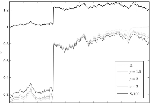
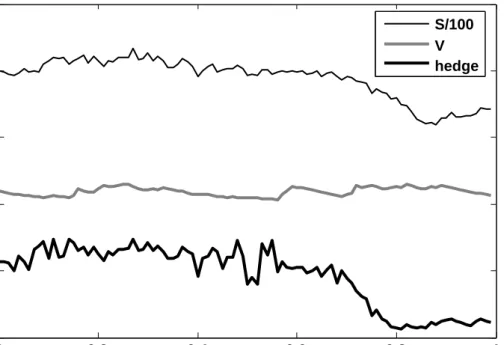
The fourth chapter presents numerical results. In this section we specify both the price process and the variance process, and set up the finite difference method to obtain a numerical solution to the partial integro-differential equation, that is needed in order to find the mean variance hedging strategy. By simulating the processes, we then find approximate mean-variance hedge ratios corresponding to the given sample paths.
Chapter 2
L´
evy processes in Finance
2.1
Introduction
In this chapter we briefly review the main properties of L´evy processes that are used in the following chapters. We introduce the geometric L´evy process and the stochastic volatility model driven by independent L´evy processes. We then consider the absolutely continuous measure changes in these models, and obtain a set of (signed) martingale measures. General reference to this section is the book by Cont and Tankov (2004), Applebaum (2004), or classic books by Jacod and Shiryaev (2002) and Sato (1999).
Definition 2.1. (L´evy process) A stochastic process X = (Xt)t≥0 with X0 = 0
a.s. is called a L´evy process if it possesses the following properties:
1. Independent increments: Xt−Xsis independent ofXv−Xu if(u, v)∩(s, t) =∅. 2. Stationary increments: the law of Xt+h−Xt does not depend on t.
3. Stochastic continuity: for all >0,limh→0P(|Xt+h−Xt| ≥) = 0.
Every L´evy process can be characterized by a triplet (A, ν, γ), where A is a symmetric nonnegative definitive d×d matrix, γ ∈ Rd and ν is a L´evy measure, meaning that ν ∈Rd and satisfies
ν(0) = 0 and Z
Rd
The following theorem shows how the triplet (A, ν, γ) is used to calculate the char-acteristic function of a L´evy process.
Theorem 2.2. (The L´evy-Khintchine representation) LetX be a L´evy process on Rd with characteristic triplet (A, ν, γ). Then
Eeihz,Xti=etψ(z), z ∈Rd ψ(z) = −1 2hz, Azi+ihγ, zi+ Z Rd (eihz,xi−1−ihz, xi1|x|≤1)ν(dx). (2.1)
Proof. cf. Cont and Tankov (2004), proof of Theorem 3.1.
Let J be a Poisson random measure associated to the jump process 4X of the L´evy processX. Its compensated measure is defined by
N(dt, dx) =J(dt, dx)−ν(dx)dt. (2.2) The next theorem shows that the sample paths of L´evy processes can be decomposed into continuous and jump parts.
Theorem 2.3. (The L´evy-Itˆo decomposition) Let X be a L´evy process. There exists b ∈ Rd, called the drift of the L´evy process, a Brownian motion B
A with covariance matrixAand an independent Poisson random measureJ onR+×(Rd−0)
such that, for every t >0, X(t) = bt+BA(t) + Z |x|<1 xN((0, t], dx) + Z |x|≥1 xJ((0, t], dx). (2.3) Proof. cf. Applebaum (2004), proof of Theorem 2.4.16.
Let us note that this decomposition is unique and b=E X(1)− Z |x|≥1 xJ((0, t], dx) .
Definition 2.4. (The L´evy stochastic integral) Let X be a L´evy process with characteristics (A, ν, γ) and L´evy-Itˆo decomposition given by (2.3). Let L = (L(t), T ≥ 0) be a square integrable predictable process, then we can construct pro-cesses with the stochastic differential
dY(t) = L(t)dX(t). (2.4)
Most of the stochastic integrals we consider will be one-dimensional L´evy-type stochastic integrals of the following form
dYt=HtdBt+ Z
R
h(t, x)N(dt, dx), (2.5) where B is now a one-dimensional standard Brownian motion. We will denote by Yc the continuous part of Y.
Theorem 2.5. (Itˆo’s formula) Let Y be a L´evy-type stochastic integral of the form (2.5). For anyf ∈C2(
R), t >0, with probability 1 we have f(Yt)−f(Y0) = Z t 0 ∂f(Yu−)dYuc+ 1 2 Z t 0 ∂2f(Yu−)d[Yc, Yc]u + Z t 0 Z R
f(Yu−+h(u, x))−f(Yu−) N(du, dx) + Z t 0 Z R f(Yu−+h(u, x))−f(Yu−)−h(u, x)∂f(Yu−) ν(dx)du = Z t 0 ∂f(Yu−)dYu+ 1 2 Z t 0 ∂2f(Yu−)d[Yc, Yc]u + X 0≤u≤t f(Yu)−f(Yu−)− 4Yu∂f(Yu−) . (2.6)
Proof. cf. Applebaum (2004), proof of Theorems 4.4.7 and 4.4.10.
Remark 2.1. The second form of Itˆo’s formula is more general and holds for any semimartingale. When the L´evy process has finite number of jumps, i.e. ν(R)<∞, one can rewrite equation (2.6) to the following form
f(Yt)−f(Y0) = Z t 0 ∂f(Yu−)dYuc+ 1 2 Z t 0 ∂2f(Yu−)d[Yc, Yc]u + X 0≤u≤t f(Yu)−f(Yu−) .
Theorem 2.6. (Martingale representation for L´evy processes) Let M be a local martingale adapted to the filtration generated by the L´evy processX. Then there exist unique pair of square integrable processes (φs, ψs) such, that Mt is represented as Mt =M0+ Z t 0 φsdBs+ Z t 0 Z R ψ(s, x)N(ds, dx), (2.7) where B is a standard Brownian motion and N is a compensated Poisson random measure of the L´evy process X.
Proof. cf. Kunita (2004), proof of Theorem 1.1.
Definition 2.7. (Orthogonality in the martingale sense) Two locally square integrable martingales M1 and M2 are called (strongly) orthogonal if M1M2 is a
local martingale, denoted by M1⊥⊥M2.
Note that there is also a notion of weak orthogonality of martingales, but when we will talk about orthogonal processes, we mean orthogonality in the strong sense. We will find the following results useful.
Proposition 2.8. (Independence of L´evy processes) Let(Xt, Yt)be a L´evy pro-cess with L´evy measure ν and without Gaussian part. Its components are indepen-dent if and only if the support of ν is contained in the set {(x, y) :xy= 0}, that is, if and only if they never jump together. In this case
ν(A) =νX(AX) +νY(AY) (2.8) where AX = {x : (x,0) ∈ A} and AY = {y : (0, y) ∈ A}, and νX and νY are L´evy measures of (Xt) and (Yt).
Proof. cf. Cont and Tankov (2004), proof of Proposition 5.3.
Definition 2.9. (Quadratic covariation) Let X and Y be two semimartingales. The quadratic covariation process [X, Y] is the semimartingale defined by
[X, Y]t =XtYt−X0Y0 − Z t 0 Xu−dYu− Z t 0 Yu−dXu. (2.9)
Definition 2.10. (Conditional quadratic covariation) Let X and Y be two semimartingales, and [X, Y] is locally of integrable variation. Then the conditional quadratic covariation hX, Yi exists and is defined to be the compensator of [X, Y].
The process [X, Y] is also called square bracket, and the processhX, Yi sharp or angle bracket.
Example 2.1. Let M1(t) and M2(t) be two local martingales with representation
kernels (φ1, ψ1) and (φ2, ψ2) from Theorem 2.6 respectively. Then
[M1, M2]t = Z t 0 φ1sφ2sds+ Z t 0 Z R ψ1(s, x)ψ2(s, x)J(ds, dx), (2.10) and hM1, M2it = Z t 0 φ1sφ2sds+ Z t 0 Z R ψ1(s, x)ψ2(s, x)ν(ds, dx). (2.11)
2.2
Stochastic exponential and exponential
mar-tingale
Let X be a general semimartingale. The adapted process that is a solution of the following stochastic integral equation
Z = 1 + Z
Z−dX, Z0 = 1, (2.12)
is called stochastic exponential or Dol´eans-Dade exponential. The continuous part of the semimartingale X is denoted by Xc. The solution to the equation (2.12) is given by Zt= exp X(t)− 1 2[X, X] c(t) Y 0≤s≤t [1 +4X(s)]e−4X(s) (2.13) for each t≥ 0, and often denoted by E(X). When we define equivalent probability measure changes, we will use the following condition
inf{4X(t), t >0}>−1 a.s.,
which guarantees positivity of the stochastic exponential. However, many interesting ”optimal” measures are only signed in general when dealing with processes with jumps, and for those we instead assume
4X(t)6=−1 a.s. for 0≤t ≤T.
In that case we can use the following characterization of semimartingales by stochas-tic exponentials.
Proposition 2.11. Let Z be a semimartingale. There exists a semimartingale X such that Z =E(X) if and only if Z0 = 1, Zt 6= 0 a.s. for 0≤ t≤ T. In that case
we can choose X :=Z−−1Z. The process X is called stochastic logarithm of Z. Proof. cf. Jacod (1979), proof of Proposition 6.5 and Exercise 6.1.
We can see from equation (2.12), that the stochastic exponential of a martingale is a local martingale. For a martingale L´evy process, the stochastic exponential is even a true martingale, cf. Proposition 1.4 in Tankov (2004). This will be important
because for ZT to be a density of a martingale measure, it needs to be a true martingale, not just a local martingale. If Z were only a local martingale measure, it could lead to pricing irregularities when pricing via expectation technique is used, cf. Cox and Hobson (2005). It is also equally important in the change of num´eraire technique, where the num´eraire is required to be a true martingale as well. The following Lemma will be useful as it provides an extension of Novikov condition for discontinuous processes, cf. Rheinl¨ander and Steiger (2006), Lemma 2.11.
Lemma 2.12. Let M be a locally bounded local P-martingale, and let Zt = E(M)t where 4M > −1. If the process
1 2hM ci t+ X s≤t (1 +4Ms) log(1 +4Ms)− 4Ms
has a predictable compensator Lt satisfying E[exp(LT)]<∞, then Z is a true mar-tingale.
However, note that the above Lemma is only useful when considering the class of probability measures as4M > −1 which assures thatZ >0.
Another interesting problem is to find a L´evy process X such that eX is a mar-tingale, then called anexponential martingale. As it will be seen in the next section, there are various ways to define models with jumps and this will show the equiva-lence between some of these models and a way to switch from one to another. The following Lemma, due to Goll and Kallsen (2000), states a sufficient condition so that the stochastic exponential of one L´evy process equals the exponential martingale of another L´evy process. Let Λ be any Borel set Λ⊂R\{0}.
Lemma 2.13. 1. Let {Xt}t≥0 be a real-valued L´evy process with characteristic
triplet (A, ν, γ) and Z = E(X) its stochastic exponential. If Z > 0 a.s. then there exists another L´evy process {Lt}t≥0 such that for all t, Zt = eLt. The process L is given by Lt= logZt=Xt− At 2 + X 0≤s≤t {log(1 +4Xs)− 4Xs}, t ≥0.
Its stochastic triplet (AL, νL, γL) is given by AL =A, νL(Λ) =ν({x: log(1 +x)} ∈Λ) = Z ∞ −∞ 1Λ(log(1 +x))ν(dx) γL =γ− A 2 + Z ∞ −∞ ν(dx){log(1 +x)1[−1,1](log(1 +x))−x1[−1,1](x)}.
2. Let{Lt}t≥0 be a real-valued L´evy process with characteristic triplet(AL, νL, γL) and St =eLt its exponential. Then there exists another L´evy process {Xt}t≥0
such that S =E(X), where Xt =Lt− At 2 + X 0≤s≤t e4Xs −1− 4L s
Its stochastic triplet (AL, νL, γL) is given by: A=AL, ν(Λ) = νL({x:ex−1} ∈Λ) = Z ∞ −∞ 1Λ(ex−1)νL(dx), γ =γL+ AL 2 + Z ∞ −∞ νL(dx){(ex−1)1[−1,1](ex−1)−x1[−1,1](x)}.
Proof. cf. Goll and Kallsen (2000), proof of Lemma A.8.
2.3
Models
Our research started off by studying the paper of Chan (1999), which provides excel-lent introduction for measure changes in the context of L´evy processes. In this paper both the minimal and the minimal entropy martingale measure are determined, and provide building blocks to study the variance-optimal and the more generalq-optimal martingale measure. The price processS in Chan (1999) is modelled by a geometric L´evy process
dSt=St−{σtdXt+btdt}, (2.14) where σt and bt are deterministic continuous functions of time, and X is a general L´evy process. The interest rates are assumed deterministic and S represents the discounted price of stocks. Using the L´evy-Itˆo decomposition, cf. Theorem 2.3, X
can by separated into its Brownian part denoted byB and the quadratic pure jump part J by writing Xt =cBt+Jt, for some c∈R. We make the following standing
Assumption 2.1. The L´evy process X satisfies R|x|≥1xν(dx)<∞.
The above assumption, together with the main assumption on the L´evy density, can be written as R(|x|2∧ |x|)ν(dx)< ∞. This will rule out L´evy process without
first moment, for example α-stable L´evy process with α < 1. But it means that there is no need to truncate large jumps. This will simplify a lot of the formulas, because it implies that one can takexas the truncation function, as opposed to the usual truncation function 1|x|≤1. In fact, X is then a special semimartingale.
Lemma 2.14. A L´evy process X is a special semimartingale if and only if it is integrable, i.e. E[X1]<∞.
Proof. cf. Kallsen (1998), proof of Lemma 2.2, 2.
Under the Assumption 2.1, the Doob-Meyer decomposition of J is given by
Jt =Nt+at, (2.15)
and using equation (2.2), we have Nt=
Z
R
x J((0, t], dx)−tν(dx), a=E(J1).
The L´evy-Khintchine formula (2.1) becomes ψ(z) = −c 2z2 2 +iaz + Z R (eizx−1−izx)ν(dx). Thus, we can rewrite (2.14) into
dSt=St−{σt(cdBt+dNt) + (aσt+bt)dt}. (2.16) An explicit solution to equation (2.16) is given by
St=S0exp Z t 0 cσsdBs+ Z t 0 σsdNs+ Z t 0 aσs+bs− c2σ2 s 2 ds × Y 0<s≤t (1 +σs4Ns) exp(−σs4Ns),
or using stochastic exponential form St=S0E Z t 0 (aσs+bs)ds+ Z t 0 cσsdBs+ Z t 0 σsdNs .
We now extend model (2.16) to include stochastic volatility, possibly with jumps as well: dSt=St− b(t, Vt−)dt+σ(t, Vt−)dBt+δ(t, Vt−)dJt dVt=g(t, Vt−)dt+γ(t, Vt−)dLt. (2.17) Here J is a pure jump L´evy process, and L is another L´evy process independent of J and of the Wiener process B. We again assume that L´evy processes J and L satisfy Assumption 2.1. For the price process S to remain non-negative, we need δ(t, Vt−)4Jt ≥ −1 for all t. Let the L´evy measure ofJ be supported on [−c1, c2] for
c1, c2 >0. Thus, in order for S to remain non-negative −1 c2 ≤δ(t, Vt−)≤ 1 c1 , for all t,
which implies that the jumps ofJ need to be bounded from below, i.e. c1 <∞, when
δ(t, Vt−) >0 for some t and bounded from above, i.e. c2 < ∞, when δ(t, Vt−) < 0 for some t. If δ changes sign in [0, T], then J needs to have compact support.
Unless stated otherwise, we assume that δ(t,·) 6= 0 and σ(t,·) 6= 0 for all t ∈
[0, T] and ν(R\0) 6= 0. We also implicitly assume that model parameters have sufficient regularity properties so that there exists unique solution to (2.17) which does not explode on [0, T], see Theorem V.38 in Protter (2004), and Assumption 3.1 in Rheinl¨ander and Steiger (2006) for general jump-diffusion model with stochastic volatility.
From now on, the quantities related to the volatility will be denoted by superscript V. For example, the L´evy-Itˆo decomposition of Lis given by
Lt =cVBtV +JtV =cVBtV + Z t 0 Z R xNV(dt, dx) +aVt.
The stock S is the only traded asset in this market. Such a market is incomplete and there are infinitely many equivalent martingale measures. Note, that market is already incomplete in the case of model (2.16) even without using stochastic
volatility. The reason for considering this kind of model is manifold. The model encompasses many uncorrelated stochastic volatility models, for example uncorre-lated Heston model, Stein and Stein model or Hull-White model are all special cases of the model considered here. From the practical point of view, the question one might ask is why to consider model that combines L´evy process with stochastic volatility. Does model with L´evy processes not provide enough flexibility over the standard geometric Brownian motion? It is well known that stochastic volatility models work best for mid to long term options. They have problems at short matu-rities as the Gaussian-based stochastic volatility models in general produce shallow implied volatility smiles, which does not correspond with the observed market im-plied smiles, see Chapter 8 in Rebonato (2004) and references therein. One reason for this is that convexity of the smile depends to some extent on the speed at which the volatility moves from its current value, which is in general not sufficient for reasonable values of volatility of volatility. On the other hand, models with jumps work better for short term options, while failing at long terms. From the calibration point of view, the combination of a L´evy driven model and stochastic volatility al-lows fitting to the implied volatility surface without needing time-dependent model parameters, see Cont and Tankov (2004). Also, Li, Wells and Yu (2006) in their study of S&P 500 returns provide an economic justification for the class of stochastic volatility models driven by infinite activity L´evy processes. They show superiority of such models in capturing the index returns over even the most sophisticated affine jump diffusion models. From theoretical point of view, the reason for considering this kind of model will become more apparent when we introduce mean-variance tradeoff process and later mean-variance hedging.
2.4
Absolutely continuous measure changes
We follow Chan (1999) and provide a characterization of all the measures Q that are absolutely continuous with respect to the physical measure P. We do this first for a geometric L´evy model (2.16) and then extrapolate to the stochastic volatility model driven by L´evy processes (2.17).
Define a process Z by Zt= exp Z t 0 HsdBs− 1 2 Z t 0 Hs2ds+ Z t 0 Z R h(s, x)N(ds, dx) × Y 0<s≤t h(s,4Js) + 1 exp −h(s,4Js) =E Z HsdBs+ Z Z R h(s, x)N(ds, dx) t t≥0, (2.18) where H is a previsible square integrable process and h(t, x) is a Borel previsible process satisfyingh(t,0) = 0 for all t ≥0.
Lemma 2.15. The process Z defined by (2.18) is a local martingale with Z0 = 1
and Z is positive if and only if h >−1. Proof. cf. Chan (1999), proof of Lemma 3.1.
Theorem 2.16. Let Q be an absolutely continuous measure with respect to P on
FT. Then there exists a martingale Z satisfying equation (2.18) such that dQ dP F T =ZT,
The variables H and h are chosen such that E[ZT] = 1. Proof. cf. Chan (1999), proof of Theorem 3.2.
Remark 2.2. Ifh >−1,Z is a positive local martingale and thus a supermartingale (a consequence of Fatou’s lemma). Moreover, if the process h in Lemma 2.15 is defined such that E[Zt] = 1 for all t, then Z is a true martingale.
Let (Ft), t ∈ [0, T] be the filtration generated by the Brownian motion Bt and the Poisson random measureJ(dt, dx). With respect to (Ft,Q) we have
1) The process ˜ Bt =Bt− Z t 0 Hsds (2.19)
is a standard Brownian motion.
2) The processJ is a quadratic pure jump process with the compensator measure ˜
that is
˜
N(dt, dx) :=J(dt, dx)−ν(dt, dx)˜ (2.21) is a martingale, or equivalently writing
˜ Nt=Nt− Z t 0 Z R xh(s, x)ν(dx)ds. (2.22) 3) Let M(t) be a Q-local martingale. Then there exists a pair of predictable processes (φt, ψ(t, x)) such that Mt is represented by
Mt =M0+ Z t 0 φsdB˜s+ Z t 0 Z R ψ(s, x) ˜N(ds, dx). (2.23) Remark 2.3. J(dt, dx) is no longer a Poisson random measure with respect toQ un-lesshis a deterministic function. Moreover, ifhis deterministic but time-dependent, then increments ofJ from equation (2.15) underQwill be independent, but not sta-tionary. If h is stochastic, the increments of J will be dependent under measure Q. Remark 2.4. In other words, ZT defines the Radon-Nikod´ym derivative of Q with respect to P. Also, note that T has to be less than infinity, which is implied by the measureQ being absolutely continuous with respect toP, otherwise the Radon-Nikod´ym derivative would be either zero or infinity, implying that the measures P and Q are mutually singular.
The following theorem will be used whenever we move from one measure to another. It provides a sufficient condition that allows separation of the jump measure from its compensator.
Theorem 2.17. If the increasing process RR
R|ψ(s, x)|J(ds, dx) (or
RR
R|ψ(s, x)|ν(ds, dx)) is locally P-integrable, then ψ is integrable with respect to the compensated measure and
Z Z R ψ(s, x)N(ds, dx) = Z Z R ψ(s, x)J(ds, dx)− Z Z R ψ(s, x)ν(ds, dx). Proof. cf. Jacod and Shiryaev (2002), Proposition II.1.28.
Using now any equivalent martingale measureQgiven by Theorem 2.16, equation (2.19) for the Brownian motion ˜B and equation (2.22) for the compensated measure
˜
N, underQ, the price process S is given by St =S0exp Z t 0 cσsdB˜s+ Z t 0 σsdN˜s+ Z t 0 aσs+cσsHs+bs− c2σ2 s 2 ds + Z t 0 σs Z R xh(s, x)ν(dx)ds Y 0<s≤t (1 +σs4N˜s) exp(−σs4N˜s).
Looking at the form of the equation above, we deduce that the general condition for the processS to be a martingale underQ is
cσsHs+aσs+bs+ Z
R
σsxh(s, x)ν(dx) = 0 for all s a.s. (2.24) It is clear that H and h are not given uniquely by the martingale condition (2.24). This is one way of seeing that the geometric L´evy model is incomplete. We will study various approaches in the next section that, in addition to (2.24), allow to specify H and h.
Moving onto the stochastic volatility model (2.17), similarly to (2.18), define the process Z by Zt=E Z HudBu+ Z Z R h(u, x)N(du, dx)+ Z FudBuV + Z Z R f(u, x)NV(ds, dx) t , (2.25)
whereH, F are previsible square integrable processes and h(t, x), f(t, x) are previs-ible processes satisfyingh(t,0) = 0 and f(t,0) = 0 for allt ≥0 and further assume that {h(t, x) = −1} and {h(t, x) = −1} are evanescent. The martingale condi-tion practically looks the same as for the geometric L´evy process, but there is now much more freedom due toF and f from (2.25) not being present in the following martingale condition: σ(s, Vs−)Hs+b(s, Vs−) +δ(s, Vs−) a+ Z R xh(s, x)ν(dx)
= 0 for all s a.s. (2.26) There is an alternative way to express the density of a martingale measure. Assum-ing that S is a special semimartingale (sufficient condition for this is for example E(|St|)<∞), S has a unique decomposition
whereM is a local martingale andA is a predictable process of finite variation. See Example 3.1 for the form ofM and A in stochastic volatility model given by (2.17). It then follows, by the absence of arbitrage, that the finite variation part A must be absolutely continuous with respect to the predictable quadratic variation of the martingale partM. This implies that there exists a predictable process ˆλsuch that
At= Z t
0
ˆ
λsdhMis,
and this is usually termed as thestructure condition. The following is a one dimen-sional version of the second claim in Proposition 2 of Schweizer (1995).
Proposition 2.18. Suppose that S satisfies the structure condition. A square-integrable local martingale Z is a martingale density for S if and only if Z satisfies the stochastic differential equation
Zt= 1−
Z t
0
ˆ
λuZu−dMu+Rt, 0≤t≤T (2.27)
for some square-integrable local martingale R strongly orthogonal to M. Proof. cf. Yoeurp and Yor (1977), proof of Theorem 2.1.
Remark 2.5. When both S andR are assumed to be locally bounded, the represen-tation (2.27) is sufficient to ensure that Q is a true martingale, see Corollary 3.2.2 of Steiger (2005). However, in the present context of L´evy processes, S and R are in general not locally bounded.
By the martingale representation property, R can be written as Rt = Z t 0 σRudBu+ Z t 0 Z R δR(u, x)N(du, dx), and asR is orthogonal to M, it satisfies
hM, Rit= Z t 0 σuσuRdu+ Z t 0 Z R δuδR(u, x)xN(du, dx) = 0. (2.28) Thus the alternative way to express the density of the martingale measure by equa-tion (2.25) satisfying the martingale condiequa-tion (2.26) is given by equaequa-tion (2.27) satisfying the orthogonality condition (2.28).
Chapter 3
Optimal martingale measures
3.1
Introduction
In the previous chapter, we have seen that the martingale condition (2.24) or (2.26) is not enough to identify a martingale measure uniquely. In this chapter, we study various additional criteria that characterize martingale measure in addition to the martingale condition. First, we determine the F¨ollmer-Schweizer minimal martin-gale measure. We then explicitly determine the variance-optimal martinmartin-gale measure and discuss cases when it is equal to the minimal martingale measure. This will have consequences in the next chapter where we study mean-variance hedging problem. We finish the chapter with the q-optimal martingale measure (q > 1), which is a generalization of the variance-optimal martingale measure for which q= 2.
We denote by Θ some space of S-integrable predictable processes (further prop-erties and requirements on Θ will be discussed later). For a positive time horizonT, the stochastic integralGT(ϑ) =
RT
0 ϑtdSt represents gains from trading according to
ϑ, which itself can be regarded as a self-financing trading strategy.
Definition 3.1. A signed martingale measure is a signed measure Q P with E dQ dP = 1 and E dQ dPGT(ϑ) = 0 for all ϑ∈Θ.
The space of all signed martingale measures will be denoted by Ms(
P). The subset ofMs(
P) of probability measures that are absolutely continuous martingale measures will be denoted byM(P), and its subset of equivalent martingale measures
will be denoted by Me( P):
M(P) ={QP:Q is a probability measure andS is a Q-local martingale},
Me
(P) ={Q∼P:Q is a probability measure andS is a Q-local martingale}. While not explicitly used in notation, note that Ms, M and Me depend on the choice of space Θ, and we need to assume that Θ contains all indicator processes 1[t1,t2[.
3.2
The minimal martingale measure
Recall that S denotes the discounted price of a stock and we assume that S is a special semimartingale with a Doob-Meyer decomposition of the form S = S0 +
M+A, where M is a local martingale andA is a process of finite variation. Under this assumption, there exists a process ˆλ such that A=R λdˆ hMi and the following process ˆ K = Z ˆ λdA= Z ˆ λ2dhMi
is called the mean-variance tradeoff process. This is nothing else than the integrated squared market price of risk. Using these notions, we can define the minimal mar-tingale measure introduced in F¨ollmer and Schweizer (1991). The density of the minimal martingale measure is given by
dPˆ dP =E − Z ˆ λdM T
providing it exists. This is the case when E−R ˆ
λdM is a uniformly integrable martingale. The ”minimal” in the name refers to the fact, that the change of measure preserves the structure of the reference measure P as much as possible in the following sense: if a square-integrable P-martingale is orthogonal to M, then it is a ˆP-martingale as well. For continuous processes, the minimal martingale measure also preserves orthogonality: if a square-integrableP-martingale is orthogonal toM, then it is orthogonal toSunder ˆPas well. However, this is no longer true whenM is not continuous, and this will play some role when we later discuss the mean-variance
and local risk-minimization hedging problems. Note also, that when the process S has jumps, E−R ˆ
λdM may become negative, and this means that the minimal martingale measure is only a signed measure in general. For further properties of the minimal martingale measure, see Schweizer (1995).
The minimal martingale measure for the geometric L´evy process was determined in Chan (1999). Here, we determine the minimal martingale measure for the stochas-tic volatility model (2.17).
Example 3.1. Stochastic volatility model. The Doob-Meyer decomposition of S is given by Mt= Z t 0 Su− σ(u, Vu−)dBu+δ(u, Vu−) Z R xN(dt, dx) , At= Z t 0 Su− δ(u, Vu−)a+b(u, Vu−) du. The mean-variance tradeoff process Kˆ is given by
ˆ Kt= Z t 0 ˆ λudAu = Z t 0 δ(u, Vu−)a+b(u, Vu−) 2 σ(u, Vu−)2 +δ(u, Vu−)2 R Rx 2ν(dx)du, (3.1) where ˆ λt= dAt dhMit = δ(u, Vu−)a+b(u, Vu−) St− σ(u, Vu−)2+δ(u, Vu−)2R Rx 2ν(dx). (3.2)
Thus density of the minimal martingale measure Pˆ is dPˆ dP =E − Z ˆ λdM T =E Z ˆ HudBu+ Z Z R ˆ h(u, x)N(du, dx) T (3.3) where ˆ Ht =−λˆtσ(t, Vt−)St−, (3.4) and ˆh(t, x) =−λˆtδ(t, Vt−)St−x. (3.5)
We will denote by Bˆt and Nˆ(dt, dx) the associated transformations of Bt and N(dt, dx) by Hˆt and ˆh(t, x), respectively, i.e.
dBˆt=dBt−Hˆtdt, (3.6) ˆ
N(dt, dx) = N(dt, dx)−h(t, x)ν(dx)dtˆ
3.3
The variance-optimal martingale measure
LetMs
2(P) denote the convex set of all signed local martingale measures with square
integrable density, ie. Ms
2(P) :=Ms(P)∩L2(P). Note thatM2s(P) is closed inL2(P)
and has a unique element with minimal L2(
P)-norm, due to convexity of the norm (provided Ms
2(P)6=∅). Thus we can define the following
Definition 3.2. Assume that M2s(P)6=∅. A signed martingale measure P˜ is called variance-optimal if P˜ minimizes dQ dP L2( P) = Var dQ dP + 1 1/2 over all Q∈Ms 2.
In this section we assume that GT(Θ) is a linear subspace of L2, which corre-sponds to a frictionless financial market (no transaction costs, taxes, etc.). The assumptions M2s(P) 6= ∅ is equivalent to assuming that 1 ∈/ GT(Θ), cf. Delbaen and Schachermayer (1996c). In the financial context, this can be regarded as a no-arbitrage condition.
Example 3.2.In this example, we calculate the explicit form of the variance-optimal martingale measureP˜ for the geometric L´evy model given by the equation (2.16). By definition dQ dP 2 L2(P) =E[ZT2] =E exp 2 Z T 0 HsdBs− Z T 0 Hs2ds+ 2 Z T 0 Z R h(s, x)N(ds, dx) × Y 0<s≤T h(s,4Xs) + 1 2 exp −2h(s,4Xs) # =E " exp Z T 0 Hs2ds−2 Z T 0 Z R h(s, x)ν(dx)ds Y 0<s≤T h(s,4Xs) + 1 2 # = exp Z T 0 Hs2ds−2 Z T 0 Z R h(s, x)ν(dx)ds ×E exp 2 Z T 0 Z R ln h(s, x) + 1J(ds, dx) , (3.8)
In the last line we used the fact that H and h are deterministic processes, which is implied by the fact that all model parameters in the martingale condition (2.24) are
deterministic themselves. Using Itˆo’s formula, it is clear that E exp 2 Z T 0 Z R ln h(s, x) + 1J(ds, dx) = exp Z T 0 Z R e2 ln(h(s,x)+1)−1ν(dx)ds . (3.9) Putting the results (3.8) and (3.9) together, we have
dQ dP 2 L2( P) = exp Z T 0 Hs2ds+ Z T 0 Z R h(s, x)2ν(dx)ds . (3.10)
To finish our example, it remains to find the explicit form of the processes H andh that minimize (3.10)subject to the martingale condition (2.24). We follow the same procedure as in Chan (1999). The most convenient way to solve this optimization problem is the use of Lagrange multipliers. First fixH, letκbe a continuous function and define the Lagrangian
L(κ, h) = Z R h(s, x)2ν(dx) + Z R κsσsh(s, x)xν(dx). (3.11) Noting that h7→L(κ, h)is convex in h, finding the value ofh that minimizes (3.11) requires d dtL(κ, h+tF) t=0 = 0 for all F, which gives
h(s, x) = −κsσsx
2 .
Plugging the optimal value of h into (2.24) and differentiating, we find that κ0s(H) = 2cσs Z R (σsx)2ν(dx) −1 . (3.12)
Turning on to minimizing H, again using the optimal value of h, we simply differ-entiate the exponent in the equation (3.10) which gives
2Hs+κ0s(H) Z
R
κs(σsx)2
2 ν(dx) = 0, and using (3.12) we find the optimal value of H to be
Hs =−σsκsc
2 .
For the sake of completeness, after using the optimal forms of H and h in (2.24), we have that κs = aσs+bs σ2 2 c2+R Rx 2ν(dx).
Comparing the results with (3.11) of Chan (1999), we see that the minimal and the variance-optimal martingale measure are exactly the same. This is always the case when the mean-variance tradeoff process process is deterministic, cf. Theorem 11 in Schweizer (1995). Another way to see this, is to look at the form of both measures. It was shown in various degrees of generality, that the density of the variance-optimal martingale measure can be written as c+R ϑdS for some c ∈ R
and ϑ∈Θ, cf. Delbaen and Schachermayer (1996c) or Schweizer (1996):
Lemma 3.3. Assume that Ms
2(P) 6=∅. Then P˜ ∈ M2s is variance-optimal, if and
only if
dP˜
dP = [1,∞) +GT(Θ). Proof. cf. Schweizer (1996), proof of Lemma 1, (c).
In the case of deterministic continuous mean-variance tradeoff
E − Z ˆ λdM =E − Z ˆ λd(S−A) =E − Z ˆ λdS EKˆ and thus both measures coincide.
Another characterization of ˜P is through the so-called adjustment process.
Definition 3.4. A processβ ∈L(S), the space of S-integrable predictable processes, is called an adjustment process if the following two conditions hold:
1. βE −R
βdS−∈Θ, 2. E[E −R
βdST GT(ϑ)] = 0 for all ϑ∈Θ.
Proposition 3.5. Assume that Ms
2(P)6=∅. If β is an adjustment process, then P˜
is given by dP˜ dP = E −R βdST E[E −R βdST] . Proof. cf. Schweizer (1996), proof of Proposition 8.
We now proceed to find ˜Pfor the stochastic volatility model (2.17) by using the above characterization. We assume the usual framework, a complete probability
space (Ω,F,F,P), with filtration F= (Ft)0≤t≤T satisfying the usual conditions gen-erated byB,J andL. Further, we assume thatS is locally inL2(P) in the following sense: there exists a sequence (τn)∞n=1of localising stopping times increasing to
infin-ity such that, for each n∈N, the family{ST :T stopping time, T ≤τn} is bounded inL2(
P), cf. Delbaen and Schachermayer (1996a).
Recall the form of ˆH and ˆhcharacterizing the minimal martingale measure, given by equations (3.4) and (3.5), respectively. For the rest of the section, we assume the following holds
Assumption 3.1. The process RR R|
ˆ
h(s, x)|J(ds, dx) is locally P-integrable. The following is a generalization of Lemma 2.15 in Biagini et al. (2000).
Proposition 3.6. Let C be a positive constant, and let F andf be predictable. The following conditions are equivalent:
a) E Z FudBVu + Z Z R f(u, x)NV(du, dx) T exp( ˆKT) =C (3.13) b) E Z ˆ HudBu+ Z Z R ˆ h(u, x)N(du, dx)+ Z FsdBuV + Z Z R f(u, x)NV(ds, dx) T = CE Z ˆ HudBˆu+ Z Z R ˆ h(u, x) ˆN(du, dx) T . (3.14)
Proof. This follows from equations (3.1), (3.4), (3.5), (3.6) and (3.7).
Remark 3.1. Equation (3.13) is a generalization of the representation equation de-rived by Biagini et al. (2000) and Hobson (2004) for diffusion stochastic volatility models and by Rheinl¨ander (2005) for the Stein and Stein model. Here the repre-sentation equation is more involved, which reflects the fact that we are dealing with a volatility process and a price process that are discontinuous.
We now move onto specifying the set of admissible strategies that we are going to use. A process ϑ is called a simple trading strategy if it has a form ϑ =h1(τ1,τ2] where τ1 < τ2 denote stopping times and h is bounded and Fτ1 measurable.
To guarantee L2(
P) closedness, we assume the following space of admissible strategies, see Delbaen and Schachermayer (1996c), Gourieroux, Laurent and Pham (1998) and the subsequent formulation of ˇCern´y and Kallsen (2007) and Xia and Yan (2006) that we use here.
Definition 3.7. A strategy ϑ ∈ L(S) is admissible, if there exists a sequence (ϑ(n))n∈N of simple trading strategies such that
Z T 0 ϑdS =L2− lim n→∞ Z T 0 ϑndS, Z t 0 ϑdS = lim n→∞ Z t 0
ϑndS in probability for all t. The space of admissible strategies is denoted by Θ.
The following result provides characterisation of admissible strategies.
Corollary 3.8. We have equivalence between: 1. ϑ is an admissible strategy
2. ϑ∈L(S), R ϑdS ∈L2(P), andZQR ϑdS is a martingale for any sigma martingale measure Q with density process ZQ and dQ
dP ∈L
2(
P).
Proof. cf. ˇCern´y and Kallsen (2007), proof of Corollary 2.5.
We also introduce alternative space of admissible strategies. For any special semimartingaleY with Doob-Meyer decompositionY =Y0+MY +AY, withM0Y =
AY 0 = 0, define kY kH2=k([MY, MY]T) 1 2 kL2( P) +kVar(A Y) T kL2( P), (3.15)
where Var(AY) denotes variation of AY. Then Y belongs to a set of square inte-grable semimartingales H2 if kY kH2<∞. We denote by ΘH the set of following strategies
ΘH :={ϑ∈L(S) : Z
ϑdS ∈H 2}.
It is in general easier to check whether certain strategy belongs to ΘH, on the other hand, as opposed toGT(Θ), the setGT(ΘH) is not necessarily closed. In this respect, a useful result is provided by Corollary 2.9 of ˇCern´y and Kallsen (2007) which shows that ΘH ⊂Θ.
Remark 3.2. In our stochastic volatility model we have k Z T 0 ˆ λdS kH2 =k( Z T 0 ˆ λ2d[M, M])12 kL2( P) +k Z T 0 |ˆλ||dA| kL2( P) =E[ Z T 0 ˆ λ2d[M, M]]12 +E[( Z T 0 ˆ λdA)2]12 =E[ Z T 0 ˆ λ2dhM, Mi]12 +E[ ˆK2 T] 1 2 =E[ ˆKT] 1 2 +E[ ˆK2 T] 1 2.
Last line implies that ˆλ ∈ ΘH if and only if the mean-variance tradeoff process ˆK has finite second moment.
We can now use the Proposition 3.6 to obtain the candidate variance-optimal martingale measure.
Lemma 3.9. Let Q be the signed local martingale measure given by dQ dP =E Z ˆ HudBu+ Z Z R ˆ h(u, x)N(du, dx) + Z FsdBuV + Z Z R f(u, x)NV(ds, dx) T
for processes F and f. Then the density of Q with respect to P is of the form dQ dP = E(− ∫λdSˆ )T E h E(− ∫λdS)ˆ T i (3.16)
if and only if the representation equation (3.13) holds with C given by C =EhE(− ∫ ˆλdS)T i−1 =E Z FudBuV + Z Z R f(u, x)NV(du, dx) T exp( ˆKT). (3.17) Proof. First assume that F and f are given by the representation equation (3.13). Note that the process S can be written as
St=S0+ Z t 0 Su− σ(u, Vu−)dBˆu+δ(u, Vu−) Z R xNˆ(du, dx) .
(3.5), imply that Z T 0 ˆ HudBuˆ + Z T 0 Z R ˆ h(u, x) ˆN(du, dx) =− Z T 0 Su−ˆλu σ(u, Vu−)dBuˆ +δ(u, Vu−) Z R xNˆ(du, dx) =− Z T 0 ˆ λudSu. This in turn implies
dQ dP =E − Z ˆ λudSu T × E Z FudBuV + Z Z R f(u, x)NV(du, dx) T exp( ˆKT), (3.18) and the representation equation (3.13) yields
dQ dP = E−R ˆ λudSu T E h E−R ˆ λudSu T i.
The proof in the other direction follows from equation (3.18) above. We can now state the main theorem of this section.
Theorem 3.10. Assume that F and f satisfy equation (3.17) and that local mar-tingale Z defined via
Zt=E Z ˆ HudBu+ Z Z R ˆ h(u, x)N(du, dx) + Z FsdBuV + Z Z R f(u, x)NV(ds, dx) t
is a true martingale. Further assume that E−R ˆ λdS
T
is square-integrable, that
E−R ˆ
λdM is integrable and that E[exp(−KˆT)]>0 P-a.s.. Then the measure Q defined via dQ/dP=ZT is the variance-optimal signed martingale measure.
Proof. By Lemma 3.9, the measureQtakes the form of the measure ˜Pfrom Propo-sition 3.5 withβ = ˆλ. The prove that Q is variance-optimal, we need to show that ˆ
λ is an adjustment process and that Ms
2(P) 6= ∅. We start by showing that the
second property of the adjustment process, c.f. Definition 3.4, holds. For anyϑ∈Θ we have E E − Z ˆ λdS T GT(ϑ) =E E − Z ˆ λdM T exp(−KˆT)GT(ϑ) (3.19)
because A is continuous and finite variation process. The expectation is finite due to square-integrability assumption of E− ∫ ˆλdS
T and the fact that ϑ∈ Θ, using Cauchy-Schwarz inequality. Now define a martingale MV
t = E[exp(−KˆT)|Ft]. As the process ˆK is independent of S, by the martingale representation theorem, cf. Theorem 2.6, we have MtV =E[exp(−KˆT)] + Z t 0 φsdBsV + Z t 0 Z R ψ(s, x)NV(ds, dx),
for some processes (φ, ψ), where integrability of MV is guaranteed by the fact that E[exp(−KˆT)|Ft]≤1. Because M is orthogonal to MV, we have
E − Z ˆ λdM T MTV =E[exp(−KˆT)]− Z T 0 MtVˆλtE − Z ˆ λdM t− dMt + Z T 0 E − Z ˆ λdM t φtdBtV + Z R ψ(t, x)NV(dt, dx)
which is by Proposition 2.18 a martingale density for S, after scaling by E[exp(−KˆT)]. Note that E
−R ˆ
λdM is a true martingale, as both Z and MV are true martingales. Thus the integrability of the product above follows from
E |E − Z ˆ λdM t MtV| ≤E |E − Z ˆ λdM t | <∞. Therefore (3.19) =E E − Z ˆ λdM T MTVGT(ϑ) = 0,
which proves the second property of the adjustment process.
We now follow the arguments of the proof of Theorem 3.3.2 in Wiese (1998) to show that the first property of the adjustment process holds. Let ¯Z be the solution to ¯Z = 1−R ˆ
λZ¯−dS. For n ∈ N, define Tn := inf{t > 0 : ˆKt ≥ n}. Consider the stopped process STn. By Protter (2004), Theorem 2.18, the stopped process ¯ZTn satisfies ¯ ZTn = 1− Z ˆ λZ¯−dSTn = 1− Z ˆ λ1[0,Tn]Z¯ Tn − dS.
In the first step we show that the integrand, ˆλ1[0,Tn]Z¯ Tn − , is admissible. We have kZ¯Tn k H2 =kZˆTnexp(−KˆTn)kH2≤kZˆTn kH2 =k Z T 0 ˆ λ21[0,Tn]( ˆZ Tn − )2d[M, M] 12 kL2( P) =E[ Z T 0 ˆ λ21[0,Tn]( ˆZ Tn − )2d[M, M]] 1 2 =E[ Z T 0 ˆ λ21[0,Tn]( ˆZ Tn − )2dhM, Mi] 1 2 ≤E[ sup t∈[0,T] ( ˆZTn t−)2 Z T 0 ˆ λ21[0,Tn]dhM, Mi] 1 2 =E[ sup t∈[0,T] ( ˆZTn t−)2KˆTTn] 1 2 = √ nE[ sup t∈[0,T] ( ˆZTn t−)2] 1 2 ≤2√nE[( ˆZTn T ) 2]12 ≤2√n E[( ¯ZTTn) 2exp(2 ˆKTn T )] 1 2 (3.20) = 2√nexp(n)E[ ¯ZTn T ] 1 2 = 2 √ nexp(n)E[ ˆZTn T exp(−Kˆ Tn T )] 1 2 (3.21) = 2√nexp(n/2). (3.22)
Line (3.20) follows from Doob’s maximal quadratic inequality, where we used the fact that ˆZ is a martingale by assumption of the Theorem. Line (3.21) is justified by using the second property of the adjustment process, which we have already proved to hold for timeT, and the fact that it holds also for the stopped process STn, due to independence of the stopping time Tn from S, i.e. E[( ¯ZTTn)2] = E[ ¯Z
Tn
T ]. Finally, (3.22) follows from the definition of the stopping time Tn and the fact that ˆZ is a martingale. Thus we have shown that ˆλ1(0,Tn]Z¯
Tn
− ∈ΘH and therefore admissible by Corollary 2.9 of ˇCern´y and Kallsen (2007). As both properties of the adjustment process hold forTn, ˆλ1(0,Tn]is the adjustment process for the stopped processS
Tnand the density of the variance-optimal martingale measure for the stopped processSTn is given by ¯ZTn T /E[ ¯Z Tn T ]. Thus ¯Z Tn T ∈L2(P) for n ∈N, {Z¯ Tn T , n ∈ N} is uniformly integrable in L2(P) and therefore E[ ¯ZTn
T ] →E[ ¯ZT], cf. Gut (2005), Theorems 5.4.2 and 5.5.2. As ˆλ1(0,Tn] is the adjustment process for the stopped process S
Tn for n∈N, we have that E[ ¯ZTn
T ]=E[( ¯Z Tn T )
2], and similarly, as the second property of the
adjustment process was shown to hold in the first part of the proof, we have that E[ ¯ZT]=E[( ¯ZT)2]. Thus E[( ¯ZTTn)2] → E[( ¯ZT)2] which by Gut (2005), Theorem 5.5.2 implies that RT 0 λ1ˆ (0,Tn]Z¯ Tn − dS converges to RT 0 λˆZ¯−dS inL 2(
P). This together with the admissibility of ˆλ1(0,Tn]Z¯
Tn
trading strategies (ϑn)
n∈Nsuch thatR0T ϑndS converges toR0T λˆZ¯−dS inL2(P). Note that all results in the proof so far also hold when T is replaced with any positive t < T. Thus we also have thatRt
0 ϑ
ndSconverges toRt
0 λˆZ¯−dSinL 2(
P) and therefore also in probability. This shows that ˆλZ¯− is admissible.
Combining the results above imply that ˆλ is an adjustment process. It only remains to show that ¯ZT/E[ ¯ZT] has finite second moment. From equation (3.17) we have that E[ ¯ZT] = E[exp(−KˆT)]. As ˆλ is an adjustment process, E[ ¯ZT] = E[ ¯ZT2]. Thus E " ¯ ZT E[ ¯ZT] 2# = E[ ¯Z 2 T] E[ ¯ZT]2 = E[ ¯ZT] E[ ¯ZT]2 = 1 E[exp(−KˆT)] ,
which is finite by assumption and therefore ¯ZT/E[ ¯ZT] is the density of the variance-optimal martingale measure.
3.3.1
Cern´
ˇ
y-Kallsen approach
We shortly comment on a different approach to determine the variance-optimal mar-tingale measure. ˇCern´y and Kallsen (2007) suggest an approach based on finding a measureP∗ that neutralizes the effect of the stochastic mean-variance tradeoff pro-cess, and the variance-optimal martingale measure is then computed as the minimal martingale measure with respect to P∗. ˇCern´y and Kallsen call P∗ the opportunity neutral measure, see Lemma 3.15 and Definition 3.16. The above can be written as
dP˜ dP = dP∗ dP dP˜ dP∗ = dP∗ dP dcP∗ dP∗.
In comparison, the approach used here is to determine the minimal martingale measure first, and in the second step the representation equation is used to determine ˜ P, dP˜ dP = dPˆ dP dP˜ dPˆ.
However in the uncorrelated case, the equation (3.27) in ˇCern´y and Kallsen (2007) that is used to characterize the opportunity process L and which in turn defines P∗, simplifies considerably. In our model, the equation (3.27) means that the drift process of the stochastic logarithm of L under P is equal to the mean-variance
tradeoff process ˆK, and going from measure P to P∗ will not change the drift of S (note that P∗ is not a martingale measure). But this implies that
dcP∗ dP∗ = dPˆ dP and dP∗ dP = dP˜ dPˆ,
ie. finding ˜P through the measure P∗ is equivalent to finding ˜P by using the repre-sentation equation, and the processLcan be recovered from the following expression
dP∗ dP =
L E[L0]E( ˆK)
3.4
The minimal entropy martingale measure
The minimal entropy martingale measure is well studied subject in the mathemat-ical finance and particularly in the context of L´evy processes, cf. Chan (1999), Frittelli (2000), Fujiwara and Miyahara (2003), Grandits and Rheinl¨ander (2002), Rheinl¨ander (1999), Rheinl¨ander (2005), Esche and Schweizer (2005), Rheinl¨ander and Steiger (2006). It has been used for pricing purposes as a martingale mea-sure with minimal relative entropy with respect to the historical probability or for calibration purposes, see for example Carr et al. (2002), Tankov (2004).
While the relative entropy is not a metric, it can be viewed as a distance between two probability measures. The relative entropy, also called Kullback–Leibler diver-gence, I(Q,P) of a probability measure Q with respect to a probability measure P is given as I(Q,P) = E dQ dP log dQ dP if QP, +∞ otherwise.
Note that I(Q,P)≥0 for any probability measure Qand I(Q,P) = 0 if and only if Q= P. The functional I(Q,P) is strictly convex in the first argument. A measure Q(e)∈M(P) which satisfies
I(Q(e),P) = min
Q∈M(P)I(Q,P)
is called theminimal entropy martingale measure.
In the exponential/geometric L´evy models, the minimal entropy martingale mea-sure preserves L´evy property. This can be seen in Chan (1999) and has been rig-orously proved in Esche and Schweizer (2005). The connection between Q(e) and
Esscher transform has been shown in Chan (1999) and further generalized and stud-ied in Fujiwara and Miyahara (2003) and Hubalek and Sgarra (2006).
Frittelli (2000) proves in Theorem 2.1 that in the case of bounded processes, the sufficient condition for existence of the minimal entropy martingale measure is existence of a martingale measure with finite relative entropy with respect to P. Moreover, if there exists an equivalent martingale measure with finite relative entropy, then the minimal entropy martingale measure is equivalent. But in the
case of unbounded processes, infQ∈M(P)I(Q,P) may not be attained by a martingale
measure.
For the remainder of this section, we assume that following holds
Assumption 3.2. S is a locally bounded.
By Proposition 3.2 of Grandits and Rheinl¨ander (2002), the density of the mini-mal entropy martingale measure Q(e) is necessary of the form
dQ(e) dP = exp c− Z T 0 λtdSt (3.23) where c is a constant and λ is a predictable process such that R λdS is a Q(e) -martingale. That (3.23) is not sufficient to characterize the martingale measure with minimal entropy has been shown by counterexample in Schachermayer (2003). Thus after finding a candidate measure Q(c), which we define to be any martingale
measure of the form (3.23), one needs to verify that the candidate measure is entropy minimizer.
Let us start by finding the candidate martingale measure. Comparing (2.25) and (3.23), we see that the candidate minimal entropy martingale measure corresponds to the choices
Ht =−λtSt−σt, (3.24) and h(t, x) = exp(−λtSt−δtx)−1. (3.25) Therefore, we define the following mapping (dependence onVt− omitted from nota-tion)
Ψ(λt, t) = −λtSt−σt2+bt+δtE(J1) +δt Z
R
x(e−λtSt−δtx−1)ν(dx) (3.26) and assume that the process λ is such that
Z
R
|x(e−λtSt−δtx−1)|ν(dx)<∞.
This guarantees that the integral in (3.26) is well defined. This will ultimately depend on how heavy are the tails of the L´evy measure. Further assume that for any t ∈ [0, T], λ is a solution to Ψ(λt, t) = 0. Note that when such λ exists, it is unique as Ψ(λt, t) is monotonically decreasing as a function of λt in its domain,
irrespective of the sign of δ. It is now a straightforward calculation to show that a local martingale measureQ(c) is of the form (3.23) if and only if F and f defined in (2.25) satisfy E Z FudBuV + Z Z f(u, x)NV(du, dx) T = exp c− 1 2 Z T 0 (σuλuSu−)2du− Z T 0 Z R e−λuSu−δux(−λ uSu−δux−1) + 1 ν(du, dx) . (3.27) The condition that guarantees the existence and uniqueness of the solution to the equation Ψ(λt, t) = 0 for all t is given in the following
Proposition 3.11. Assume that J satisfies the following condition
Z {|x|≥1}
euxν(dx)<∞, for any u∈(−u1, u2), where 0< u1, u2 ≤ ∞.
Then the equation Ψ(λt, t) = 0 has a unique solution for all t. If furthermore bt+δtE(J1)>0, then λt∈ 0,bt+δtE(J1) St−σt2 . Proof. It follows from the assumption that
Z {|x|≥1}
xγeuxν(dx)<∞ ∀γ >0.
which implies that the integral in the definition of Ψ(λt, t) is finite for λt ∈ (−u2/(St−δt), u1/(St−δt)) when δt >0 and for λt ∈ (u1/(St−δt),−u2/(St−δt)) when δt < 0, and thus Ψ(λt, t) is well defined. For a fixed t, Ψ(λt, t) is monotonically decreasing as a function of λt (irrespective of the sign of δt). Moreover,
lim λ↓− u2 St−δt Ψ(λ, t) = ∞ and lim λ↑ u1 St−δt Ψ(λ, t) =−∞ for δt>0, lim λ↓ u1 St−δt Ψ(λ, t) =∞ and lim λ↑ −u2 St−δt Ψ(λ, t) = −∞ forδt<0.
Thus equations of the form Ψ(λ,·) =const have unique solution for all λ for which Ψ(λ,·)<∞.
For the second assertion, note that Ψ(0, t) = bt + δtE(J1) and for λt = bt+δtE(J1)
St−σ2t
, only the integral part in the expression of Ψ(q, λ, t) is non-zero. How-ever, because the integral part is monotonically decreasing in λt (irrespective of the
sign of δt) and it is zero at λt = 0, the integral part and thus Ψ(q, λ, t) must be negative at λt =
bt+δtE(J1)
St−σ2t
because of the assumption bt +δtE(J1) > 0. This
implies thatλt lies in the interval
0,bt+δtE(J1) St−σt2
.
The following is the Proposition 3.2, Grandits and Rheinl¨ander (2002), which ensures that the candidate measure Q(c) minimizes the entropy.
Proposition 3.12. Assume there exists Q(c) ∈ Me(
P) such that H(Q(c),P) < ∞. Then Q(c) =
Q(e) if and only if the following hold: (i) dQ(c)/d
P=cexp((− ∫ λdS)T) for a constant c and an S-integrable λ; (ii) EQ[(− ∫ λdS) T] = 0 for Q=Q(c),Q(e). Obviously I(Q(e),P) = logE exp −1 2 Z (σuλu)2du− Z Z e−λuδux(−λ uδux−1) + 1 ν(du, dx) =c.
For L´evy processes, we know that the stochastic exponential of a martingale is in fact a martingale, cf. Proposition 1.4 in Tankov (2004). But in general it is only a local martingale. As the minimal entropy martingale measure is a probability mea-sure, one can use Lemma 2.12 to guarantee that Q(c) is a true martingale measure.
When S is locally bounded, a sufficient condition forR
λdS to be aQ(e)-martingale
is provided by Proposition 3.2 of Rheinl¨ander (2005). In our case this condition translates to E exp Z T 0 λ2tSt2− (σ(t, Vt−)2dt+δ(t, Vt−)2 Z R x2J(dx, dt) <∞. (3.28) This implies thatR λdS is a true Q-martingale for allQ∈Me(
P), and thus Q(c) = Q(e) by Proposition 3.12. Note that (3.28) involves the unknown λ. From the second statement of Proposition 3.11, we have upper bound forλ2 and thus we have the following alternative sufficient condition to (3.28), that involves only model parameters: E exp Z T 0 (bt+δtE(J1))2 σ(t, Vt−)4 (σ(t, Vt−)2dt+δ(t, Vt−)2 Z R x2J(dx, dt) <∞. (3.29)
The Proposition 3.12 assumes that there exists equivalent martingale measure with finite entropy. By appealing to the result of Frittelli (2000), Theorem 2.1, we can provide a condition which guarantees that there exists a unique minimal entropy martingale measure. It is sufficient, for example, if the minimal martingale measure has finite entropy. The entropy of the minimal martingale measure is given by
E " dPˆ dPlog dPˆ dP # = ˆE " log d ˆ P dP # = ˆE Z T 0 ˆ HudBˆu+ 1 2 Z T 0 ˆ Hu2du+ Z T 0 Z R ˆ h(u, x) ˆN(du, dx) + Z T 0 Z R ˆ h(u, x)2ν(dx)du+ Z T 0 Z R
log(ˆh(u, x) + 1)−ˆh(u, x)ν(du, dx)ˆ =E 1 2 Z T 0 ˆ Hu2du+ Z T 0 Z R
log(ˆh(u, x) + 1)−ˆh(u, x) ˆh(u, x) + 1ν(dx)du
. The last line follows from the fact that the model parameters depend only on the volatility process, which has the same distribution under both measure P and the minimal martingale measure ˆP. Therefore, if
E 1 2 Z T 0 ˆ Hu2du+ Z T 0 Z R
log(ˆh(u, x) + 1)−ˆh(u, x) ˆ
h(u, x) + 1
ν(dx)du
<∞, the minimal entropy martingale measure exists.
3.5
The
q
-optimal martingale measure
In this section we consider a set of signed martingale measures of which the variance-optimal martingale measure is a special case. Let q > 1 and p be its conjugate, namely 1
p + 1
q = 1. Similarly to the previous section, we denote by M s
q(P) :=
Ms(
P)∩Lq(P) andMqe(P) :=Me(P)∩Lq(P). Note that Mqs(P) is closed in Lq(P) and has a unique element with minimal Lq(P)-norm, due to convexity of the norm (provided Ms
q(P)6=∅). Thus we can define the following
Definition 3.13. Assume that Mqs(P) 6= ∅. A signed martingale measure Q(q) is called q-optimal if Q(q) minimizes Lq(
P)-norm, i.e. E dQ(q) dP q = inf Q∈Mqs(P) E dQ dP q .
In the context of stochastic volatility models driven by two correlated Brownian motions, the q-optimal martingale measure was studied in Hobson (2004) through the fundamental representation equation, which provides characterisation of the q-optimal martingale measure with respect to the real world measure. More recently, several authors studied this problem in the models with jumps. Jeanblanc, Kl¨oppel and Miyahara (2007) provide sufficient conditions to identify the q-optimal martin-gale measure for exponential L´evy processes, however the authors do not consider signed martingale measures, only equivalent ones. For this reduced optimisation problem, they show that it suffices to consider equivalent martingale measures that preserve the L´evy property and this reduces the problem to a deterministic convex optimization problem. In Bender and Niethammer (2007), theq-optimal signed mar-tingale measure is identified in the exponential L´evy models, and the proof is based on a hedging argument and duality for convex optimisation. The authors restrict the values ofq toq = 2m2m−1 for somem∈N, and they also study the convergence of the q-optimal signed martingale measures to the minimal entropy martingale measure. In the general semimartingale model, under some assumptions, the q-optimal mar-tingale measure and q-optimal hedging problem was studied in Arai (2006). Also, in Sabanis (2008), necessary and sufficient conditions for the candidate measure to be q-optimal are presented.