Selection of our books indexed in the Book Citation Index in Web of Science™ Core Collection (BKCI)
Interested in publishing with us?
Contact [email protected]
Numbers displayed above are based on latest data collected. For more information visit www.intechopen.com Open access books available
Countries delivered to Contributors from top 500 universities International authors and editors
Our authors are among the
most cited scientists
Downloads
We are IntechOpen,
the world’s leading publisher of
Open Access books
Built by scientists, for scientists
12.2%
122,000
135M
TOP 1%
154
Online Incremental Face Recognition System
Using Eigenface Feature and Neural Classifier
Seiichi Ozawa
1, Shigeo Abe
1, Shaoning Pang
2and Nikola Kasabov
21
Graduate School of Engineering, Kobe University,
2Knowledge Engineering & Discover Research Institute, Auckland University of Technology
1
Japan,
2New Zealand
1. Introduction
Understanding how people process and recognize faces has been a challenging problem in the field of object recognition for a long time. Many approaches have been proposed to simulate the human process, in which various adaptive mechanisms are introduced such as neural networks, genetic algorithms, and support vector machines (Jain et al., 1999). However, an ultimate solution for this is still being pursued. One of the difficulties in the face recognition tasks is to enhance the robustness over the spatial and temporal variations of human faces. That is, even for the same person, captured images of human faces have full of variety due to lighting conditions, emotional expression, wearing glasses, make-up, and so forth. And the face features could be changed slowly and sometimes drastically over time due to some temporal factors such as growth, aging, and health conditions.
When building a face recognition system, taking all the above variations into consideration in advance is unrealistic and maybe impossible. A remedy for this is to make a recognition system evolve so as to make up its misclassification on its own. In order to construct such an adaptive face recognition system, so-called incremental learning should be embedded into the system because it enables the system to conduct learning and classification on an ongoing basis. One challenging problem for this type of learning is to resolve so-called “plasticity and stability dilemma” (Carpenter & Grossberg, 1988). Thus, a system is required to improve its performance without deteriorating classification accuracy for previously trained face images. On the other hand, feature extraction plays an essential role in pattern recognition because the extraction of appropriate features results in high generalization performance and fast learning. In this sense, incremental learning should be considered not only for a classifier but also for the feature extraction part. As far as we know, however, many incremental learning algorithms are aiming for classifiers. As for the incremental learning for feature extraction, Incremental Principal Component Analysis (IPCA) (e.g., Oja & Karhunen, 1985; Sanger, 1989; Weng et al., 2003; Zhao et al., 2006) and Incremental Linear Discriminant Analysis (Pang et al., 2005; Weng & Hwang, 2007) have been proposed so far. Hall and Martin (1998) proposed a method to update eigen-features (e.g., eigen-faces) incrementally based on eigenvalue decomposition. Ozawa et al. (2004) extended this IPCA algorithm such that an eigen-axis was augmented based on the accumulation ratio to control the dimensionality of an eigenspace easily.
Open
Access
Database
www.intechweb.org
Recently, a prototype face recognition system was developed by the authors (Ozawa et al, 2005) based on a new learning scheme in which a classifier and the feature extraction part were simultaneously learned incrementally. In this system, IPCA was adopted as an online feature extraction algorithm, and Resource Allocating Network with Long-Term Memory (RAN-LTM) (Kobayashi et al., 2001) was adopted as a classifier model. It was verified that the classification accuracy of the above classification system was improved constantly even if a small set of training samples were provided at a starting point. To accelerate learning of IPCA, we also proposed an extended algorithm called Chunk IPCA (Ozawa et al., 2008) in which an eigenspace is updated for a chunk of given training examples by solving a single intermediate eigenvalue problem.
The aim of this chapter is to demonstrate the followings:
1. how the feature extraction part is evolved by IPCA and Chunk IPCA,
2. how both feature extraction part and classifier are learned incrementally on an ongoing basis,
3. how an adaptive face recognition system is constructed and how it is effective.
This chapter is organized as follows. In Section 2, IPCA is first reviewed, and then Section 3 presents the detailed algorithm of Chunk IPCA. Section 4 explains two neural classifier models: Resource Allocating Network (RAN) and its variant model called RAN-LTM. In Section 5, an online incremental face recognition system and its information processing are described in detail, and we also explain how to reconstruct RAN-LTM when an eigenspace model is dynamically updated by Chunk IPCA. In Section 6, the effectiveness of incremental learning in face recognition systems is discussed for a self-compiled face image database. Section 7 gives conclusions of this chapter.
2. Incremental Principal Component Analysis (IPCA)
2.1 Learning assumptions and outline of IPCA algorithm
Assume that N training samples i n
R
∈
) (
x (i=1,…,N) are initially provided to a system and an eigenspace model Ω=(x,Uk,Λk,N) is obtained by applying Principal Component Analysis (PCA) to the training samples. In the eigenspace model Ω,
x
is a mean vector of) (i
x (i =1,…,N), Uk is an n×k matrix whose column vectors correspond to eigenvectors, and Λk =diag
{
λ
1,…,λ
k}
is a k×kmatrix whose diagonal elements are non-zero eigenvalues. Here,k
is the number of eigen-axes spanning the eigenspace (i.e., eigenspace dimensionality) and the value of k is determined based on a certain criterion (e.g., accumulation ratio). After calculating Ω, the system keeps the information on Ω and all the training samples are thrown away.Now assume that the (N +1)th training sample x(N+1) =y ∈Rn is given. The addition of this new sample results in the changes in the mean vector and the covariance matrix; therefore, the eigenspace model Ω=(x,Uk,Λk,N) should be updated. Let us define the
new eigenspace model by Ω′=(x′,U′k′,Λ′k′,N +1). Note that the eigenspace dimensions
might be increased from k to k+1; thus, k′ in Ω′ is either k or k+1. Intuitively, if almost all energy of y is included in the current eigenspace spanned by the eigenvectors U′k, there
is no need to increase an eigen-axis. However, if y includes certain energy in the complementary eigenspace, the dimensional augmentation is inevitable; otherwise crucial information on y might be lost. Regardless of the necessity in eigenspace augmentation, the
eigen-axes should be rotated to adapt to the variation in the data distribution. In summary, there are three main operations in IPCA: (1) mean vector update, (2) eigenspace augmentation, and (3) eigenspace rotation. The first operation is easily carried out without past training examples based on the following equation:
(
x y)
x + + = ′ N N 1 1 n R ∈ . (1)Hence, the following subsections give the explanation only for the last two operations.
2.2 Eigenspace augmentation
There have been proposed two criteria for judging eigenspace augmentation. One is the norm of a residue vector defined by
g U x y
h=( − )− kT where g=UkT(y−x). (2) Here, T means the transposition of vectors and matrices. The other is the accumulation ratio whose definition and incremental calculation are shown as follows:
∑
∑
∑
∑
= = = = − + + − + + = = n j j k i T k i n j j k i i k N N A 1 2 1 2 1 1 ) 1 ( ) ( ) 1 ( ) ( x y x y U Uλ
λ
λ
λ
(3)where
λ
i is the ith largest eigenvalues, n and k mean the dimensionality of the input space and that of the current eigenspace, respectively. The former criterion in Eq. (2) was adopted in the original IPCA (Hall & Martin, 1998), and the latter in Eq. (3) was used in the modified IPCA proposed by the authors (Ozawa et al., 2004). Based on these criteria, the condition of increasing an eigen-axis hˆ is represented by:[Residue Vector Norm]
⎩ ⎨ ⎧ > = otherwise 0 if / ˆ h h h
η
h (4) [Accumulation Ratio] ⎩ ⎨ ⎧ < = otherwise 0 ) ( if / ˆ h h A Ukθ
h (5)where
η
(in the original IPCA,η
is set to zero) andθ
are positive constants. Note that setting a too large thresholdη
or too smallθ
would cause serious approximation errors for eigenspace models. Hence, it is important to set proper values toη
in Eq. (4) andθ
in Eq. (5). In general, finding a proper thresholdη
is not easy unless input data are appropriately normalized within a certain range. On the other hand, since the accumulation ratio is defined by the ratio of input energy in an eigenspace over the original input space, the value ofθ
is restricted between 0 and 1. Therefore, it would be easier forθ
to get an optimal value by applying the cross-validation method. The detailed algorithm of findingθ
in incremental learning settings is described in Ozawa et al. (2008).2.3 Eigenspace rotation
If the condition of Eq. (4) or (5) satisfies, the dimensions of the current eigenspace would be increased from k to k+1, and a new eigen-axis hˆ is added to the eigenvector matrix Uk. Otherwise, the dimensionality remains the same. After this operation, the eigen-axes are rotated to adapt to the new data distribution. Assume that the rotation is given by a rotation matrix R, then the eigenspace update is represented by the following equation:
1) If there is a new eigen-axis to be added, U′k+1 =[Uk,hˆ]R, (6)
2) otherwise, U′k =Uk R. (7) It has been shown that R is obtained by solving the following intermediate eigenproblem (Hall & Martin, 1998):
1. If there is a new eigen-axis to be added,
, ) 1 ( 0 1 2 2 = ′+1 ⎪⎭ ⎪ ⎬ ⎫ ⎪⎩ ⎪ ⎨ ⎧ ⎥ ⎦ ⎤ ⎢ ⎣ ⎡ + + ⎥ ⎦ ⎤ ⎢ ⎣ ⎡ + T k T T k N N N N Λ R R g g gg 0 0 Λ
γ
γ
γ
(8) 2. otherwise, . ) 1 ( 1 2 k T k N N N N Λ R R gg Λ = ′ ⎭ ⎬ ⎫ ⎩ ⎨ ⎧ + + + (9)Here,
γ
=hˆT(y−x) and 0 is a k-dimensional zero vector; Λ′k+1 and Λ′k are the new eigenvalue matrices whose diagonal elements correspond to k and k+1 eigenvalues, respectively. Using the solution R, the new eigenvector matrix U′k or U′k+1 is calculated from Eq. (6) or (7).3. Chunk Incremental Principal Component Analysis (Chunk IPCA)
3.1 Learning assumptions and outline of chunk IPCA algorithm
IPCA can be applied to one training sample at a time, and the intermediate eigenproblem in Eq. (8) or (9) must be solved for each sample even though a chunk of samples are provided to learn at a time. Obviously this is inefficient from a computational point of view, and the learning may get stuck in a deadlock if a large chunk of training samples is given to learn in a short term; that is, the next chunk of training samples could come before the learning is completed if it takes long time for updating an eigenspace.
To overcome this problem, the original IPCA is extended so that the eigenspace model Ω can be updated with a chunk of training samples in a single operation (Ozawa et al., 2008). This extended algorithm is called Chunk IPCA.
Assume again that N training samples
{
(1) ( )}
, , x N xX= … ∈Rn×N have been given so far and an eigenspace model Ω=(x,Uk,Λk,N) was obtained from these samples. Now, a chunk of
L training samples
{
(1) ( )}
, , y L yY= … ∈Rn×L are presented to the system. Let the updated eigenspace model be Ω′=(x′,U′k′,Λ′k′,N +L). The mean vector x′ in Ω′ can be updated
(
x y)
x N L L N + + = ′ 1 . (10)The problem is how to update U′k and Λ′k in Ω′.
As shown in the derivation of IPCA, the update of U′k and Λ′k is reduced to solving an
intermediate eigenproblem, which is derived from an eigenvalue problem using a covariance matrix. Basically, the intermediate eigenproblem for Chunk IPCA can also be derived in the same way as shown in the derivation of IPCA (Hall & Martin, 1998). However, we should note that the dimensionality k′ of the updated eigenspace could range from k to k+L depending on the given chunk data Y. To avoid constructing a redundant eigenspace, the smallest k′ should be selected under the condition that the accumulation ratio is over a designated threshold. Thus, an additional operation to select a smallest set of eigen-axes is newly introduced into Chunk IPCA. Once the eigen-axes to be augmented are determined, all the eigen-axes should be rotated to adapt to the variation in the data distribution. This operation is basically the same as in IPCA.
In summary, there are three main operations in Chunk IPCA: (1) mean vector update, (2) eigenspace augmentation with the selection of a smallest set of eigen-axes, and (3) eigenspace rotation. The first operation is carried out by Eq. (10). The latter two operations are explained below.
3.2 Eigenspace augmentation
In Chunk IPCA, the number of eigen-axes to be augmented is determined by finding the minimum
k
such that A(Uk)≥θ
holds whereθ
is a threshold between 0 and 1. Tointroduce this criterion, we need to modify the update equation of Eq. (3) such that the accumulation ratio can be updated incrementally for a chunk of L samples. In Chunk IPCA, we need to consider two types of accumulation ratios. One is the accumulation ratio for a k -dimensional eigenspace spanned by U′k =UkR where R is a rotation matrix which is calculated from the intermediate eigenvalue problem described later. The other is that for a (k+l)-dimensional augmented eigenspace spanned by U′k+l =
[
Uk,Hl]
R where Hl is a set ofl augmented eigen-axes. The former is used for checking if the current k-dimensional eigenspace should be augmented or not. The latter one is used for checking if further eigen-axes are needed for the (k+l)-dimensional augmented eigenspace.
The new accumulation ratio A′(U′k) and A′(U′k+l) are calculated as follows (Ozawa et al.,
2008):
∑
∑
∑
∑
= = = = ′′ + + + ′′ + + + = ′ ′ n i L j j i k i L j j i k N L N L N L N L A 1 1 2 2 1 1 2 2 1 1 ) ( μ μ g g Uλ
λ
(11)∑
∑
∑
∑
= = = = + ′′ + + + ′′ ′′ + + + ≈ ′ ′ n i L j j i k i L j j j i l k N L N L N L N L A 1 1 2 2 1 1 2 2 1 1 ) ( μ μ γ g γ g Uλ
λ
(12)where g =UTk
(
y−x)
, gi′′=UkT(
y(i) −y)
, μ=x−y, ( ) , y y μ′′ = j − j γ=H(
y−x)
, T l and(
y y)
H γ′′= T (i) − li . To update A′(U′k), the summation of eigenvalues
λ
i (i =1,…,n) isrequired, and this summation can be held by accumulating the power of training samples (Ozawa et al., 2004). Hence, the individual eigenvalues
λ
i (i= k+1,…,n) are not necessary for this update.As seen from Eqs. (11) and (12), we need no past sample
x
(j) and no rotation matrix R to update the accumulation ratio. Therefore, this accumulation ratio is updated with the following information: a chunk of given training samples{
(1) ( )}
, , y L y
Y= … , the current eigenspace model Ω=(x,Uk,Λk,N), the summation of eigenvalues
∑
=n
j 1
λ
i , and a set ofaugmented eigen-axes Hl which are obtained through the procedure described next. In IPCA, a new eigen-axis is obtained to be orthogonalized to the existing eigenvectors (i.e., column vectors of Uk). A straightforward way to obtain new eigen-axes is to apply
Gram-Schmidt orthogonalization to a chunk of given training samples (Hall et al., 2000). If the training samples are represented by L~ linearly independent vectors, the maximum number of augmented eigen-axes is L~. However, the subspace spanned by all of the L~ eigen-axes is redundant in general. Therefore, we should find a smallest set of eigen-axes without losing essential information on Y.
The problem of finding an optimal set of eigen-axes is stated below.
Find the smallest set of eigen-axes
{
1, , *}
*
l
h h
H = … for the current eigenspace model
) , , , (x Uk Λk N =
Ω without keeping the past training samples X such that the accumulation ratio
) ( k l*
A′ U′+ of all the given training samples
{
X,Y}
is larger than a thresholdθ
.Assume that we have a candidate set of augmented eigen-axes Hl =
{
h1,…,hl}
. Since thedenominator of Eq. (12) is constant once the mean vector
y
is calculated, the increment of the accumulation ratio from A′(U′k) to A′(U′k+l) is determined by the numerator terms.Thus, let us define the following difference ΔA~′(Uk′+l) of the numerator terms between ) ( k A′ U′ and A′(U′k+l):
∑
∑
= = + = + − + − Δ ′ ′ ′ Δ l i i L j j T l T l l k A N L N L A 1 def 1 2 ) ( 2 ~ ) ( 1 ) ( ) ( ~ y y H y x H U (13) where{
( )}
1{
( )}
. ~ 1 2 ) ( 2∑
= − + − + = ′ Δ L j j T i T i i N L N L A h x y h y y (14)Equation (13) means that the increments of the accumulation ratio is determined by the linear sum of ΔA~i′. Therefore, to find the smallest set of eigen-axes, first we find hi with the largest ΔA~i′, and put it into the set of augmented eigen-axes Hl (i.e., l =1 and Hl =hi). Then, check if the accumulation ratio A′(U′k+l) in Eq. (12) becomes larger than the threshold
θ
. If not, select hi with the second largest ΔA~i′, and the same procedure is repeated untilθ
≥ ′ ′( k+l)
A U satisfies. This type of greedy algorithm makes the selection of eigen-axes very
3.3 Eigenspace rotation
Next, let us derive the update equations for Uk and Λk. Suppose that l eigen-axes are
augmented when a chunk of L training samples Y is provided; that is, the eigenspace dimensions are increased by l. Let us denote the augmented eigen-axes as follows:
{
1, ,}
Rn l, 0 l L. l l = ∈ ≤ ≤ × h h H … (15)Then, the updated eigenvector matrix U′k+l is represented by R
H U
U′k+l =[ k, l] (16)
where R is a rotation matrix. It has been shown that Ris obtained by solving the following intermediate eigenproblem (Ozawa et al., 2008):
1. If there are new eigen-axes to be added (i.e., l ≠0),
⎪⎩ ⎪ ⎨ ⎧ ⎥ ⎦ ⎤ ⎢ ⎣ ⎡ ′ ′ ′ ′ ′ ′ ′ ′ + + ⎥ ⎦ ⎤ ⎢ ⎣ ⎡ + + ⎥ ⎦ ⎤ ⎢ ⎣ ⎡ +
∑
= L i T i i T i i T i i T i i T T T T T k L N N L N NL L N N 1 3 2 3 2 ) ( ) ( 0 γ g γ γ γ g g g γ γ g γ γ g g g 0 0 Λ, ) ( ) 2 ( 1 3 k l L i T i i T i i T i i T i i L N N L L + = ′ = ⎪⎭ ⎪ ⎬ ⎫ ⎥ ⎦ ⎤ ⎢ ⎣ ⎡ ′′ ′′ ′′ ′′ ′′ ′′ ′′ ′′ + +
∑
R RΛ γ γ g γ γ g g g (17) 2. otherwise, . ) ( ) 2 ( ) ( ) ( 1 1 3 3 2 3 2 k L i L i T i i T i i T k L N N L L L N N L N NL L N N Λ R R g g g g g g Λ = ′ ⎭ ⎬ ⎫ ⎩ ⎨ ⎧ ′′ ′′ + + + ′ ′ + + + + +∑
=∑
= (18) Here, g′i =UTk(
y(i) −x)
and γ′ =H(
y −x)
) (i T li . As seen from Eqs. (17) and (18), the rotation
matrix R and the eigenvalue matrix Λ′k+l correspond to the eigenvectors and eigenvalues of the intermediate eigenproblem, respectively. Once R is obtained, the corresponding new eigenvector matrix Uk′+l is given by Eq. (16).
The overall algorithm of Chunk IPCA is summarized in Algorithm 2.
3.4 Training of initial eigenspace
Assume that a set of initial training samples D
{
( (i), (i))|i 1, ,N}
0= x z = … is given before
incremental learning gets started. To obtain an initial eigenspace model Ω=(x,Uk,Λk,N),
the conventional PCA is applied to D0 and the smallest dimensionality k of the eigenspace is
determined such that the accumulation ratio is larger than θ. Since a proper θ is usually unknown and often depends on training data, the cross-validation technique can be applied to determining θ (Ozawa et al., 2008). However, for the sake of simplicity, let us assume here that a proper θ is given in advance. The algorithm of the initial training is shown in Algorithm 3.
4. Incremental learning of classifier
4.1 Resource Allocating Network (RAN)
Resource Allocating Network (RAN) (Platt, 1991) is an extended version of RBF networks. When the training gets started, the number of hidden units is set to one; hence, RAN has simple approximation ability at first. As the training proceeds, the approximation ability of RAN is developed with the increase of training samples by allocating additional hidden units.
Figure 1 illustrates the structure of RAN. The output of hidden units
{
}
T Jy y1,…,
=
y is
calculated based on the distance between an input x=
{
x1,…,xI}
T and center vector of the jth hidden unit{
}
T jI j j = c 1,…,c c : 2 2 exp j for 1, , j j y j Jσ
⎛ − ⎞ ⎜ ⎟ = − = ⎜ ⎟ ⎝ ⎠ … x c (19)where I and J are the numbers of input units and hidden units, respectively, and 2
j
σ
is a variance of the jth radial basis. The network output z ={
z1,…,zK}
T is calculated as follows:K k y w z k K k j kj k for 1, , 1 … = + =
∑
=γ
(20)where K is the number of output units, wkj is a connection weight from the jth hidden unit
to the kth output unit, and
γ
k is a bias of the kth output unit.When a training sample (x,d) is given, the network output is calculated based on Eqs. (19) and (20), and the root mean square error E = d−z between the output z and target d for the input x is evaluated. Depending on E, either of the following operations is carried out:
c
Jc
2c
1 Input Layer Hidden Layerx (t)
Ix (t)
1x (t)
2y (t)
1y (t)
2y (t)
J Output Layerz (t)
1z (t)
Kw
11w
1Jw
K1w
KJ1. If E is larger than a positive constant
ε
and the distance between an input x and its nearest center vector *c is larger than a positive value
δ
(t) (i.e., E>ε
and) ( * t
δ
> −cx ), a hidden unit is added (i.e., J ←J+1). Then, the network parameters for the Jth hidden unit (center vector cJ, connection weights wJ =
{
w1J,…,wKJ}
, and variance 2j
σ
) are set to the following values: cJ =xp, wJ =d − z , and*
c x−
=
κ
σ
Jwhere
κ
is a positive constant.δ
(t) is decreased with time t as follows:⎥ ⎦ ⎤ ⎢ ⎣ ⎡ ⎟ ⎠ ⎞ ⎜ ⎝ ⎛ −
=max max exp , min )
(
δ
τ
δ
δ
t t (21)where
τ
is a decay constant,δ
max andδ
min are maximum and minimum values of) (t
δ
, respectively.2. Otherwise, the network parameters are updated as follows:
pj k OLD kj NEW kj w e y w = +
α
(22)∑
= − + = K k kj k pj ji pi j OLD ji NEW ji c x c y e w c 1 2 ( )σ
α
(23) k OLD k NEW kγ
α
eγ
= + (24)where ek =dk −zk and
α
is a positive learning ratio.Although the approximation ability is developed by allocating hidden units, the interference cannot be suppressed completely only by this mechanism. In the next section, we present an extended model of RAN in which a mechanism of suppressing the interference is explicitly introduced.
4.2 Resource allocating network with long-term memory
RAN is a neural network with spatially localised basis functions; hence it is expected that the catastrophic interference (Carpenter & Grossberg, 1988) is alleviated to some extent. However, since no explicit mechanism of suppressing the interference is introduced, the insufficient suppression might cause serious unlearning over the long run.
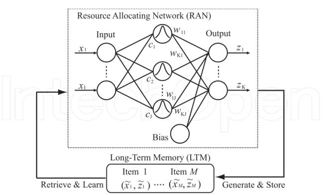
To suppress unexpected forgetting in RAN, Resource Allocating Network with Long-Term Memory (RAN-LTM) (Kobayashi et al., 2001) has been proposed. Figure 2 shows the architecture of RAN-LTM which consists of two modules: RAN and an external memory called Long-Term Memory (LTM). Representative input-output pairs are extracted from the mapping function acquired in RAN and they are stored in LTM. These pairs are called
memory items and some of them are retrieved from LTM to learn with training samples. In the learning algorithm, a memory item is created when a hidden unit is allocated; that is, an RBF center and the corresponding output are stored as a memory item.
Retrieve & Learn Generate & Store Long-Term Memory (LTM) Item 1 Item M
....
(
x
1,
z
1)
~
~
(
x
M,
z
M)
~
~
Resource Allocating Network (RAN)
c
1c
2x
1w
11w
1Jw
K1w
KJz
1x
Iz
Kc
J Input Output BiasFig. 2. Architecture of RAN-LTM.
The learning algorithm of RAN-LTM is divided into two phases: the allocation of hidden units (i.e., incremental selection of RBF centers) and the calculation of connection weights between hidden and output units. The procedure in the former phase is the same as that in the original RAN, except that memory items are created at the same time. Once hidden units are allocated, the centers are fixed afterwards. Therefore, the connection weights W=
{ }
wjkare only parameters that are updated based on the output errors. To minimize the errors based on the least squares method, it is well known that the following linear equations should be solved (Haykin, 1999):
D
ΦW = (25)
where D is a matrix whose column vectors correspond to the target outputs and Φ is a matrix of hidden outputs. Suppose that a new training sample (x,d) is given and M
memory items (~x(m),~z(m)) (m=1,…,M) have already been created, then in the simplest version of RAN-LTM (Ozawa et al., 2005) the target matrix D are formed as follows:
{
,~(1), ,~(M)}
T.z z
d
D= … Furthermore, Φ=
{ }
φ
ij (i=1,…,M +1) is calculated from the training sample and memory items as follows:). , , 1 ; , , 1 ( ~ exp , exp 2 2 , 1 2 2 1 j J i M j j i j i j j j = … = … ⎟⎟ ⎟ ⎠ ⎞ ⎜⎜ ⎜ ⎝ ⎛ − − = ⎟⎟ ⎟ ⎠ ⎞ ⎜⎜ ⎜ ⎝ ⎛ − − = +
σ
φ
σ
φ
x c x c (26)Singular Value Decomposition (SVD) can be used for solving W in Eq. (25). The learning algorithm of RAN-LTM is summarized in Algorithm 4.
5. Face recognition system
Figure 3 shows the overall process in the proposed face recognition system. As seen from Fig. 3, the proposed system mainly consists of the following four sections: face detection, face recognition, face image verification, and incremental learning. The information processing in each section is explained below.
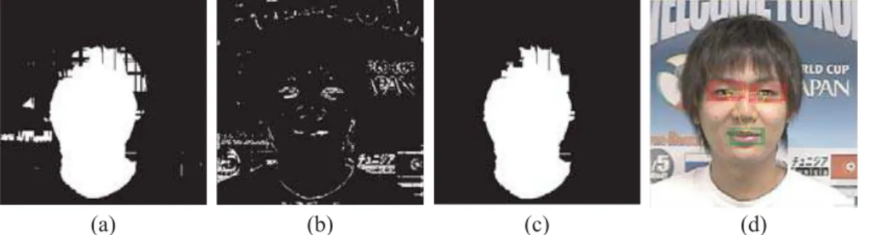
5.1 Face detection
In the face detection part, we adopt a conventional algorithm that consists of two operations: face localization and face feature detection. Figure 4 shows an example of the face detection process.
Facial regions are first localized in an input image by using the skin color information and horizontal edges. The skin color information is obtained by projecting every pixel in the input image to a skin-color axis. This axis was obtained from Japanese skin images in advance. In our preliminary experiment, the face localization works very well with 99% accuracy for a Japanese face database.
Face Localization Face Recognition Input Images Detected Faces Misclassified Images Facial Feature Detection DNN VNN Face Image Verification Face Detection Feature Extraction RNN Classification Check Result Incremental Learning Training Images Verified Faces
Fig. 3. The processing flow in the face recognition system. DNN and VNN are implemented by RBF networks, while RNN is implemented by RAN-LTM that could learn misclassified face images incrementally. In the feature extraction part, an eigen-space model is
incrementally updated for misclassified face images by using Chunk IPCA.
(a) (b) (c) (d)
Fig. 4. The process of face detection: (a) an output of skin colour filter and (b) an output of edge filter, (c) a face region extracted from the two filter outputs in (a) and (b), and (d) the final result of the face detection part. Only one face was detected in this case.
After the face localization, three types of facial features (eye, nose, mouth) are searched for within the localized regions through raster operations. In each raster operation, a small sub-image is separated from a localized region. Then, the eigen-features of the sub-sub-image are given to Detection Neural Network (DNN) to verify if it corresponds to one of the facial features. The eigenspace model for the face detection part was obtained by applying PCA to a large image dataset of human eye, nose, and mouth in advance. This dataset is also used for the training of DNN.
After all raster operations are done, face candidates are generated by combining the identified facial features. All combinations of three facial features are checked if they satisfy a predefined facial geometric constraint. A combination of three features found on the geometric template qualifies as a face candidate. The output of the face detection part is the center position of a face candidate.
The overall process in the face detection part is summarized in Algorithm 5.
5.2 Face recognition and face image verification
In the face recognition part, all the detected face candidates are classified into registered or non-registered faces. This part consists of the following two operations: feature extraction and classification (see Fig. 3). In the feature extraction part, the eigenface approach is adopted here to find informative face features. A face candidate is first
projected to the eigen-axes to calculate eigen-features, and they are given to RAN-LTM called Recognition Neural Network (RNN). Then, the classification is carried out based on the outputs of RNN.
If the recognition is correct, RNN should be unchanged. Otherwise, RNN must be trained with the misclassified images to be classified correctly afterward. The misclassified images are collected to carry out incremental learning for both feature extraction part and classifier (RNN). Since the perfect face detection cannot be always ensured, there is a possibility that non-face images happen to be mixed with the misclassified face images. Apparently the training of these non-face images will deteriorate the recognition performance of RNN. Thus, another RBF network called Verification Neural Network (VNN) is introduced into this part in order to filter non-face images out.
5.3 Incremental learning
Since face images of a person can vary depending on various temporal and special factors, the classifier should have high adaptability to those variations. In addition, the useful features might also change over time for the same reason. Therefore, in the face recognition part, the incremental learning should be conducted for both feature extraction part and classifier.
The incremental learning of the feature extraction part is easily carried out by applying Chunk IPCA to misclassified face images. However, the incremental learning of classification part (RNN) cannot be done in a straightforward manner due to the learning of the eigenspace model. That is to say, the inputs of RNN would dynamically change not only in their values but also in the number of input variables due to the eigen-axis rotation and the dimensional augmentation in Chunk IPCA. Therefore, to make RNN adapt to the change in the feature extraction part, not only the network parameters (i.e., weights, RBF centers, etc.) but also its network structure have to be modified.
Under one-pass incremental learning circumstances, this reconstruction of RNN is not easily done without unexpected forgetting of the mapping function that has been acquired so far. If the original RAN is adopted as a classifier, there is no way of retraining the neural classifier to ensure that all previously trained samples can be correctly classified again after the update of the feature space because the past training samples are already thrown away. This can be solved if a minimum number of representative samples are properly selected and used for retraining the classifier. RAN-LTM is suitable for this purpose.
To implement this idea, we need to devise an efficient way to adapt the memory items in RAN-LTM to the updated eigenspace. Let an input vector of the mth memory item be
I m R ∈ ) ( ~
x and let its target vector be m K
R ∈ ) ( ~z :
{
( ) ~( )}
, ~m m z x (m=1,…,M). Furthermore, let the original vector associated with ~x(m) in the input space be x(m)∈Rn. The two input vectors have the following relation: ~x(m) =UT(x(m)−x). Now, assume that a new eigenspace model Ω′=(x′,U′k+l,Λ′k+l,N +L) is obtained by applying Chunk IPCA to a chunk of Ltraining samples Y =(y1,…,yL). Then, the updated memory item ~x(m)' should satisfy the following equation:
) ( 1 1 ) ( ) ( ' ~( ) ( ) ( ) y x U x x U x x U x ′ − + + − ′ = ′ − ′ = + + T+ l k m T l k m T l k m N (27)
where x′ and U′k+l are given by Eqs. (10) and (16), respectively. The second term in the
right-hand side of Eq. (27) is easily calculated. To calculate the first term exactly, however, the information on x(m), which is not usually kept in the system for reasons of memory
efficiency, is needed. Here, let us consider the approximation to the first term without keeping x(m).
Assume that l of eigen-axes Hl is augmented. Substituting Eq. (16) into the first term on the
right-hand side of Eq. (27), then the first term is reduced to
⎥ ⎦ ⎤ ⎢ ⎣ ⎡ − = − ′+ ) ( ~ ) ( ( ) ) ( ) ( x x H x R x x U T m l m T m T l k . (28)
As seen from Eq. (28), we still need the information on x(m) in the subspace spanned by the
eigen-axes in Hl. This information was lost during the dimensional reduction process. The
information loss caused by this approximation depends on how a feature space evolves throughout the learning. In general, the approximation error depends on the presentation order of training data, the data distribution, and the threshold θ for the accumulation ratio in Eqs. (11) and (12). In addition, the recognition performance depends on the generalization performance of RNN; thus, the effect of the approximation error for memory items is not easily estimated in general. However, recalling a fact that the eigen-axes in Hl are orthogonal to every
vector in the subspace spanned by Uk, the error could be small if an appropriate threshold θ is
selected. Then, we can approximate the term HTl (x(m)−x) to zero, and Eq. (27) is reduced to
) ( 1 1 0 ~ ' ~( ) ( ) y x U x R x ′ − + + ⎥ ⎦ ⎤ ⎢ ⎣ ⎡ ≈ T m T m N (29)
Using Eq. (29), memory items in RNN can be recalculated without keeping the memory items m n
R
∈
) (
x in the input domain even after the eigenspace model is updated by Chunk IPCA. Then, RNN, which is implemented by RAN-LTM, is retrained with L training samples and M updated memory items
{
~(m)',~(m)'}
z
x (m=1,…,M) based on Algorithm 4. The procedure of incremental learning is summarized in Algorithm 7.
5.4 Overall algorithm of online incremental face recognition system
As mentioned in Section 5.1, the eigenspace model for the face detection part is obtained by applying PCA to a large dataset of human eye, nose, and mouth images. This dataset is used for training DNN as well. The training of VNN is carried out using a different dataset which includes a large amount of face and non-face images. Note that DNN and VNN are trained based on the learning algorithm of RAN (see Section 2). All the trainings for the face detection part, DNN, and VNN are conducted in advance.
Finally, we summarize the overall algorithm of the proposed online incremental face recognition system in Algorithm 8.
6. Performance evaluation
6.1 Experimental Setup
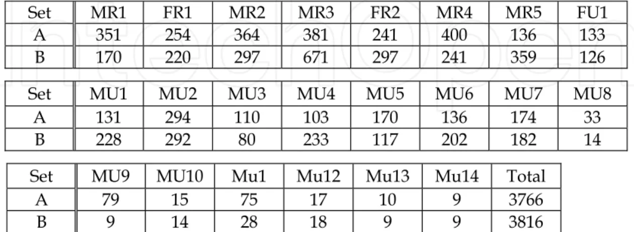
To simulate real-life environments, 224 video clips are collected for 22 persons (19 males / 3 females) during about 11 months such that temporal changes in facial appearances are included. Seven people (5 males / 2 females) are chosen as registrants and the other people (14 males /a female) are non-registrants. The duration of each video clip is 5-15 (sec.). A video clip is given to the face detection part, and the detected face images are automatically forwarded to the face recognition part. The numbers of detected face images are summarized in Table 1. The three letters in Table 1 indicate the code of the 22 subjects in which M/F and R/U mean Male/Female and Registered/Unregistered, respectively; for example, the third registered male is coded as MR3.
The recognition performance is evaluated through two-fold cross-validation; thus, the whole dataset is subdivided into two subsets: Set A and Set B. When Set A is used for learning RNN, Set B is used for testing the generalization performance, and vice versa. Note that since the incremental learning is applied only for misclassified face images, the recognition accuracy before the incremental learning is an important performance measure. Hence, there are at least two performance measures for the training dataset: one is the performance of RNN using a set of training samples given at each learning stage, and the other is the performance using all
training datasets given so far after the incremental learning is carried out. In the following, let us call the former and latter datasets as incremental dataset and training dataset, respectively. Besides, let us call the performances over the incremental dataset and training dataset as
incremental performance and training performance, respectively. We divide the whole dataset into 16 subsets, each of which corresponds to an incremental dataset. Table 2 shows the number of images included in the incremental datasets.
Set MR1 FR1 MR2 MR3 FR2 MR4 MR5 FU1 A 351 254 364 381 241 400 136 133 B 170 220 297 671 297 241 359 126 Set MU1 MU2 MU3 MU4 MU5 MU6 MU7 MU8
A 131 294 110 103 170 136 174 33 B 228 292 80 233 117 202 182 14 Set MU9 MU10 Mu1 Mu12 Mu13 Mu14 Total
A 79 15 75 17 10 9 3766 B 9 14 28 18 9 9 3816 Table 1. Two face datasets (Set A and Set B) for training and test. The three letters in the upper row mean the registrant code and the values in the second and third rows are the numbers of face images.
Set 1 2 3 4 5 6 7 8 A 220 232 304 205 228 272 239 258 B 288 204 269 246 273 270 240 281 Set 9 10 11 12 13 14 15 16 A 212 233 290 212 257 188 199 217 B 205 249 194 241 214 226 210 206 Table 2. Number of images included in the 16 incremental datasets.
Stage Init. 1 2 … 12 13 14 15
Case 1 1 2 3 … 13 14 15 16
Case 2 1,2 3 4 … 14 15 16 ---
Case 3 1,2,3 4 5 … 15 16 --- ---
Table 3. Three series of incremental datasets. The number in Table 2 corresponds to the tag number of the corresponding incremental dataset.
MR3
FR2
MR4
Learning Stages
init. 2 4 6 8 11 13
The size of an initial dataset can influence the test performance because different initial eigen-spaces are constructed. However, if the incremental learning is successfully carried out, the final performance should not depend on the size of the initial dataset. Hence, the three different series of incremental datasets shown in Table 3 are defined to see the influence. Note that the number in Table 3 corresponds to the tag number (1-16) of the incremental dataset in Table 2. Hence, we can see that Case 1 has 15 learning stages and the number of images in the initial dataset is 220 for Set A and 288 for Set B, which correspond to 6.7% and 7.5% over the whole data. On the other hand, the sizes of the initial datasets in Case 2 and Case 3 are set to a larger value as compared with that in Case 1; while the numbers of learning stages are smaller than that in Case 1. Figure 6 shows the examples of detected face images for three registered persons at several learning stages.
When an initial dataset is trained by RNN, the number of hidden units is fixed with 50 in this experiment. The other parameters are set as follows:
σ
2 =7,ε
=0.01, andδ
=5. The thresholdθ
of the accumulation ratio in IPCA is set to 0.9; thus, when the accumulation ratio is below 0.9, new eigen-axes are augmented.6.2 Experimental results
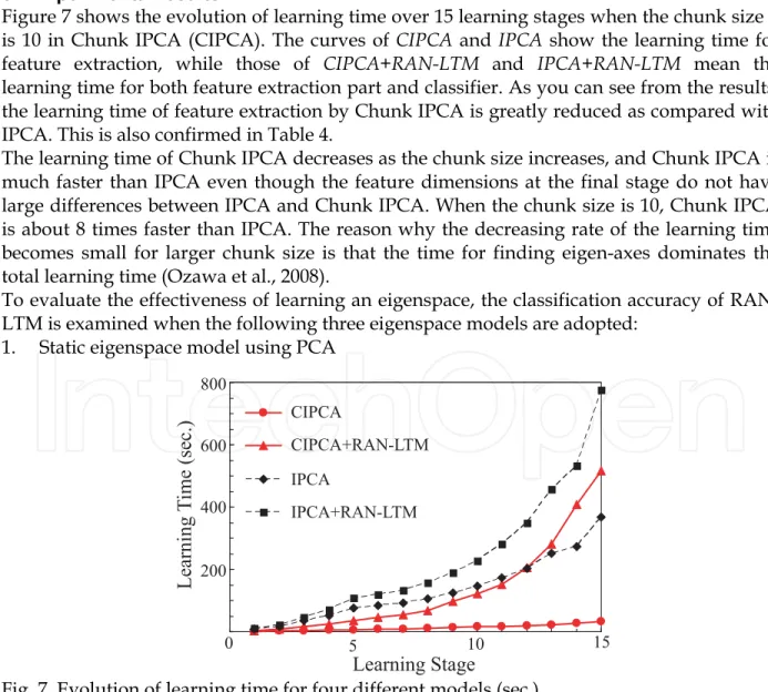
Figure 7 shows the evolution of learning time over 15 learning stages when the chunk size L
is 10 in Chunk IPCA (CIPCA). The curves of CIPCA and IPCA show the learning time for feature extraction, while those of CIPCA+RAN-LTM and IPCA+RAN-LTM mean the learning time for both feature extraction part and classifier. As you can see from the results, the learning time of feature extraction by Chunk IPCA is greatly reduced as compared with IPCA. This is also confirmed in Table 4.
The learning time of Chunk IPCA decreases as the chunk size increases, and Chunk IPCA is much faster than IPCA even though the feature dimensions at the final stage do not have large differences between IPCA and Chunk IPCA. When the chunk size is 10, Chunk IPCA is about 8 times faster than IPCA. The reason why the decreasing rate of the learning time becomes small for larger chunk size is that the time for finding eigen-axes dominates the total learning time (Ozawa et al., 2008).
To evaluate the effectiveness of learning an eigenspace, the classification accuracy of RAN-LTM is examined when the following three eigenspace models are adopted:
1. Static eigenspace model using PCA
5 10 15 0 200 400 600 800 CIPCA CIPCA+RAN-LTM IPCA IPCA+RAN-LTM Learning Stage Learning T ime (sec.)
IPCA CIPCA(10) CIPCA(50) CIPCA(100) Time (sec.) 376.2 45.6 22.5 18.1
Dimensions 178 167 186 192
Table 4. Comparisons of Learning time and dimensions of feature vectors at the final
learning stage. CIPCA(10), CIPCA(50), and CIPCA(100) stand for Chunk IPCA in which the chunk sizes are set to 10, 50, and 100, respectively.
2. Adaptive eigenspace model using the extended IPCA 3. Adaptive eigenspace model using Chunk IPCA.
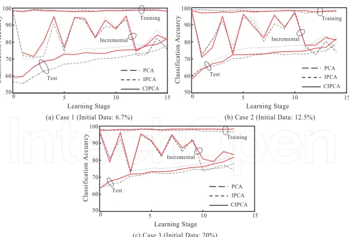
Figures 8 (a)-(c) show the evolution of recognition accuracy over 15 learning stages when the percentage of initial training data is (a) 6.7%, (b) 12.5%, and (c) 20%, respectively. As stated before, the size of an initial dataset can influence the recognition accuracy because different eigenspaces are constructed at the starting point. As seen from Figs. 8 (a)-(c), the initial test performance at stage 0 is higher when the number of initial training data is larger; however, the test performance of IPCA and Chunk IPCA is monotonously enhanced over the learning stages and it reaches almost the same accuracy regardless of the initial datasets. Considering that the total number of training data is the same among the three cases, we can say that the information on training samples is stably accumulated in RNN without serious forgetting even though RNN is reconstructed all the time the eigenspace model is updated. In addition, the test performance of RNN with IPCA and Chunk IPCA has significant improvement against RNN with PCA. This result shows that the incremental learning of a
10 15 50 100 60 70 80 90 5 0 PCA IPCA CIPCA Test Incremental Training Learning Stage Classification Accuarcy
(a) Case 1 (Initial Data: 6.7%)
PCA IPCA CIPCA Test Incremental Training 100 60 70 80 90 Classification Accuarcy 10 15 50 5 0 Learning Stage (b) Case 2 (Initial Data: 12.5%)
PCA IPCA CIPCA 100 60 70 80 90 Classification Accuarcy 10 15 50 5 0 Learning Stage (c) Case 3 (Initial Data: 20%)
Test
Incremental
Training
Fig. 8. Evolution of recognition accuracy for three different datasets (incremental, training, test) over the learning stages when the percentages of initial training datasets are set to (a) 6.7%, (b) 12.5%, and (c) 20.0%.
feature space is very effective to enhance the generalization performance of RNN. However, Chunk IPCA has slightly lower performance than IPCA. It is considered that this degradation originates from the approximation error of the eigenspace model using Chunk IPCA.
In Figs. 8 (a)-(c), we can see that although the incremental performance is fluctuated, the training performance of RNN with IPCA and Chunk IPCA changes very stably over the learning stages. On the other hand, the training performance of RNN with PCA rather drops down as the learning stage proceeds. Since the incremental performance is defined as a kind of test performance for the incoming training dataset, it is natural to be fluctuated. The important result is that the misclassified images in the incremental dataset are trained stably without degrading the classification accuracy for the past training data.
From the above results, it is concluded that the proposed incremental learning scheme, in which Chunk IPCA and RAN-LTM are simultaneously trained in an online fashion, works quite well and the learning time is significantly reduced by introducing Chunk IPCA into the learning of the feature extraction part.
7. Conclusions
This chapter described a new approach to constructing adaptive face recognition systems in which a low-dimensional feature space and a classifier are simultaneously learned in an online way. To learn a useful feature space incrementally, we adopted Chunk Incremental Principal Component Analysis in which a chunk of given training samples are learned at a time to update an eigenspace model. On the other hand, Resource Allocating Network with Long-Term Memory (RAN-LTM) is adopted as a classifier model not only because incremental learning of incoming samples is stably carried out, but also because the network can be easily reconstructed to adapt to dynamically changed eigenspace models.
To evaluate the incremental learning performance of the face recognition system, a self-compiled face image database was used. In the experiments, we verify that the incremental learning of the feature extraction part and classifier works well without serious forgetting, and that the test performance is improved as the incremental learning stages proceed. Furthermore, we also show that Chunk IPCA is very efficient compared with IPCA in term of learning time; in fact, the learning speed of Chunk IPCA was at least 8 times faster than IPCA.
8. References
Carpenter, G. A. and Grossberg, S. (1988). The ART of Adaptive Pattern Recognition by a Self-organizing Neural Network, IEEE Computer, Vol. 21, No. 3, pp. 77-88.
Hall, P. & Martin, R. (1998). Incremental Eigenanalysis for Classification, Proceedings of British Machine Vision Conference, Vol. 1, pp. 286-295.
Hall, P. Marshall, D. & Martin, R. (2000). Merging and Splitting Eigenspace Models, IEEE Trans. on Pattern Analysis and Machine Intelligence, Vol. 22, No. 9, pp. 1042-1049. Jain, L. C., Halici, U., Hayashi, I., & Lee, S. B. (1999). Intelligent Biometric Techniques in
Fingerprint and Face Recognition, CRC Press.
Kasabov, N. (2007). Evolving Connectionist Systems: The Knowledge Engineering Approach, Springer, London.
Kobayashi, M., Zamani, A., Ozawa, S. & Abe, S. (2001). Reducing Computations in Incremental Learning for Feedforward Neural Network with Long-term Memory,
Proceedings of Int. Joint Conf. on Neural Networks, Vol. 3, pp. 1989-1994.
Oja, E. & Karhunen, J. (1985). On Stochastic Approximation of the Eigenvectors and Eigenvalues of the Expectation of a Random Matrix, J. Math. Analysis and Application, Vol. 106, pp. 69-84.
Ozawa, S., Pang, S., & Kasabov, N. (2004) A Modified Incremental Principal Component Analysis for On-line Learning of Feature Space and Classifier. In: PRICAI 2004: Trends in Artificial Intelligence, Zhang, C. et al. (Eds.), LNAI, Springer-Verlag, pp. 231-240.
Ozawa, S., Toh, S. L., Abe, S., Pang, S., & Kasabov, N. (2005). Incremental Learning of Feature Space and Classifier for Face Recognition, Neural Networks, Vol. 18, Nos. 5-6, pp. 575-584.
Ozawa, S., Pang, S., & Kasabov, N. (2008). Incremental Learning of Chunk Data for On-line Pattern Classification Systems, IEEE Trans. on Neural Networks, Vol. 19, No. 6, pp. 1061-1074.
Pang, S., Ozawa, S. & Kasabov, N. (2005). Incremental Linear Discriminant Analysis for Classification of Data Streams, IEEE Trans. on Systems, Man, and Cybernetics, Part B, Vol. 35, No. 5, pp. 905-914.
Sanger, T. D. (1989). Optimal Unsupervised Learning in a Single-layer Linear Feedforward Neural Network, Neural Networks, Vol. 2, No. 6, pp. 459-473.
Weng, J., Zhang Y. & Hwang, W.-S. (2003). Candid Covariance-Free Incremental Principal Component Analysis, IEEE Trans. on Pattern Analysis and Machine Intelligence, Vol. 25, No. 8, pp. 1034-1040.
Weng, J. & Hwang, W.-S. (2007). Incremental Hierarchical Discriminant Regression, IEEE Trans. on Neural Networks, Vol. 18, No. 2, pp. 397-415.
Zhao, H., Yuen, P. C. & Kwok, J. T. (2006). A Novel Incremental Principal Component Analysis and Its Application for Face Recognition, IEEE Trans. on Systems, Man and Cybernetics, Part B, Vol. 36, No. 4, pp. 873-886.
ISBN 978-3-902613-42-4 Hard cover, 436 pages
Publisher I-Tech Education and Publishing Published online 01, January, 2009 Published in print edition January, 2009
InTech Europe
University Campus STeP Ri Slavka Krautzeka 83/A 51000 Rijeka, Croatia Phone: +385 (51) 770 447 Fax: +385 (51) 686 166 www.intechopen.com
InTech China
Unit 405, Office Block, Hotel Equatorial Shanghai No.65, Yan An Road (West), Shanghai, 200040, China Phone: +86-21-62489820
Fax: +86-21-62489821
Notwithstanding the tremendous effort to solve the face recognition problem, it is not possible yet to design a face recognition system with a potential close to human performance. New computer vision and pattern recognition approaches need to be investigated. Even new knowledge and perspectives from different fields like, psychology and neuroscience must be incorporated into the current field of face recognition to design a robust face recognition system. Indeed, many more efforts are required to end up with a human like face recognition system. This book tries to make an effort to reduce the gap between the previous face recognition research state and the future state.
How to reference
In order to correctly reference this scholarly work, feel free to copy and paste the following:
Seiichi Ozawa, Shigeo Abe, Shaoning Pang and Nikola Kasabov (2009). Online Incremental Face Recognition System Using Eigenface Feature and Neural Classifier, State of the Art in Face Recognition, Julio Ponce and Adem Karahoca (Ed.), ISBN: 978-3-902613-42-4, InTech, Available from:
http://www.intechopen.com/books/state_of_the_art_in_face_recognition/online_incremental_face_recognition_ system_using_eigenface_feature_and_neural_classifier