Nonparametric estimation for stochastic differential
equations with random effects
Fabienne Comte, Valentine Genon-Catalot, Adeline Samson
To cite this version:
Fabienne Comte, Valentine Genon-Catalot, Adeline Samson. Nonparametric estimation for stochastic differential equations with random effects. Stochastic Processes and their Applica-tions, Elsevier, 2013, 123 (7), pp.2522-2551. <10.1016/j.spa.2013.04.009>. <hal-00761394>
HAL Id: hal-00761394
https://hal.archives-ouvertes.fr/hal-00761394
Submitted on 5 Dec 2012HAL is a multi-disciplinary open access archive for the deposit and dissemination of sci-entific research documents, whether they are pub-lished or not. The documents may come from teaching and research institutions in France or abroad, or from public or private research centers.
L’archive ouverte pluridisciplinaire HAL, est destin´ee au d´epˆot et `a la diffusion de documents scientifiques de niveau recherche, publi´es ou non, ´emanant des ´etablissements d’enseignement et de recherche fran¸cais ou ´etrangers, des laboratoires publics ou priv´es.
EQUATIONS WITH RANDOM EFFECTS
F. COMTE(1), V. GENON-CATALOT(1) & A. SAMSON(1)
Abstract. We considerN independent stochastic processes(Xj(t), t∈[0, T]), j= 1, . . . , N,
defined by a one-dimensional stochastic differential equation with coefficients depending on a random variableφjand study the nonparametric estimation of the density of the random effect
φjin two kinds of mixed models. A multiplicative random effect and an additive random effect are successively considered. In each case, we build kernel and deconvolution estimators and study their L2-risk. Asymptotic properties are evaluated as N tends to infinity for fixed T
or for T =T(N)tending to infinity with N. ForT(N) =N2, adaptive estimators are built. Estimators are implemented on simulated data for several examples.
December 5, 2012
Keywords and phrases: Diffusion process, mixed models, nonparametric estimation, random ef-fects.
AMS Classification. 62G07–62M05.
Running title: Estimation for SDE with random effects.
(1): Sorbonne Paris Cité, MAP5, UMR 8145 CNRS, Université Paris Descartes, FRANCE, email: [email protected],
1. Introduction
Random effects models are increasingly used in the biomedical field and have proved to be adequate tools for the study of repeated measurements collected on a series of subjects (seee.g.
Davidian and Giltinian, 1995, Pinheiro and Bates, 2000, Nie and Yang, 2005, Nie, 2006, 2007). Such mixed models are defined through a hierarchical structure where, first, a distribution describes the intra-individual variability and, second, a distribution describes the inter-individual variability. In stochastic differential equations (SDEs) with random effects, the dynamics of each individual is given by a SDE with drift and/or diffusion coefficient depending on parameters, and the parameters of each SDE are random variables thus taking into account the variability between individuals. To be more precise, consider the following one-dimensional SDE modeling a continuous evolution forN subjects:
(1) dXj(t) =b(Xj(t), φj)dt+σ(Xj(t), φj)dWj(t), Xj(0) =xj, j= 1, . . . , N.
Here,x1, . . . , xN are known values,(W1, . . . , WN) are independent standard Brownian motions,
φ1, . . . , φN are i.i.d. random variables and (W1, . . . , WN) and (φ1, . . . , φN) are independent.
Each process(Xj(t))represents an individual and the random variableφj represents the random
effect of individual j. The functions b(x, ϕ), σ(x, ϕ) are supposed to be known and statistical inference is mainly concerned with the common unknown distribution of the random effects
φj. In several recent contributions, a parametric model is proposed for the latter distribution
and various numerical as well as theoretical results have been obtained concerning maximum likelihood estimation (see e.g. Ditlevsen and De Gaetano, 2005, Overgaardet al., 2005, Donnet and Samson, 2008, Picchiniet al., 2010, Picchini and Ditlevsen, 2011, Donnet and Samson, 2010, Delattreet al., 2012).
Nonparametric estimation in the context of random effects models has been recently investi-gated for linear discrete time models (seee.g. Comte and Samson, 2012). To our knowledge, the problem of nonparametric estimation of the population distribution (distribution of φj) has not been yet investigated in the context of SDEs with random effects. In this paper, we study this topic in two special cases of (1). First, a multiplicative random effect in the drift:
(2) dXj(t) =φj b(Xj(t))dt+σ(Xj(t))dWj(t), Xj(0) =xj, j= 1, . . . , N.
Second, an additive random effect in the drift:
(3) dXj(t) = (φj+ b(Xj(t)))dt+σ(Xj(t))dWj(t), Xj(0) =xj, j = 1, . . . , N.
The functions b : R → R and σ : R → R are known. We assume that the random variables
φ1, . . . , φN have a common density f on R and that the processes (Xj(t)) are continuously
observed on a time interval[0, T]withT >0given. We build a series of nonparametric estimators of the density f from the observations {Xj(t),0≤t ≤T, j = 1, . . . , N} which are either kernel or deconvolution estimators. We study theL2-risk of the proposed estimators and discuss their
asymptotic properties asN tends to infinity. We distinguish the case of fixedT and the case of
T =T(N) tending to infinity with N. In view of practical implementation, the case of discrete observations (Xj(kδ),0 ≤k ≤n, j = 1, . . . , N), with nδ =T is studied. Numerical simulation results using discretized sample paths for various models are given.
Section 2 concerns model (2). For large T, we propose a kernel estimator fˆh(1) of f. The bound of its L2-risk shows that T =T(N) ≥N3 ensures the possibility of obtaining the usual optimal rates on Nikol’ski classes of regularity for f. Section 2.2 is devoted to the special case
b = σ. Using an approach analogous to the one in Comte and Samson (2012), we build a deconvolution estimator fˆm(2) and discuss its properties for fixed and large T. Then, under the
conditionT =T(N) =N2, a special class of deconvolution estimators( ˆf
We propose a data-driven selection of the parameter τ which is non standard and leads to an adaptive estimator (Theorem 1).
Section 3 concerns model (3). We follow an analogous scheme. The model assumptions and the constraints on T are weaker. First, a kernel estimator fˆh(4) is proposed which attains usual optimal rates for T = T(N) ≥ N5/2. Then, for T = T(N) = N2 a class of deconvolution
estimators ( ˜fτ, τ ≤N2))and a data-driven selection of τ are studied.
In view of practical implementation, we consider the case of discrete observations with small sampling interval δ and check that the estimators can be adapted to this case (Section 4). This is used indeed in Section 5, devoted to numerical simulation on various models: the kernel and the adaptive deconvolution estimators are implemented. The results are satisfactory, even when the condition T(N) =N2 is not fulfilled. In Section 6, model properties are investigated in the
general framework of (1) or in the special cases of (2) and (3). Some concluding remarks are given in Section 7. Proofs are gathered in Section 8.
2. Multiplicative random effect in the drift
We consider in this section model (2) whereϕbelongs toRand band σ are known functions satisfying:
(H1) b andσ are Lipschitz:
∃L >0,∀x, y∈R, |b(x)−b(y)|+|σ(x)−σ(y)| ≤L|x−y|. (H2) Z T 0 b2 σ2(Xj(s))ds <+∞, j= 1, . . . , N, a.s.
The processes (W1, . . . , WN) and the r.v.’s (φ1, . . . , φN) are defined on a common probability
space (Ω,F,P). Consider the filtration (Ft, t ≥ 0) defined by Ft = σ(φj, Wj(s), s ≤ t, j =
1, . . . , N). As Ft=σ(Wi(s), s≤t)∨ Fi
t, withFti =σ(φi,(φj, Wj(s), s≤t), j 6=i) independent
of Wi, each process Wi is a (Ft, t ≥ 0)-Brownian motion. The random variables φi are F0
-measurable. Under (H1), equation (2) admits a strong solution adapted to the filtration(Ft, t≥ 0)(see Proposition 8). Assumption (H2) is clearly fulfilled, for instance, if σ is lower bounded. Following Delattreet al. (2012), we may now introduce statistics which have a central role in the estimation procedure. For j= 1, . . . , N, we denote
(4) Uj(t) = Z t 0 b σ2(Xj(s))dXj(s), Vj(t) = Z t 0 b2 σ2(Xj(s))ds.
Then, equation (2) yields:
(5) Uj(t) =φjVj(t) +Mj(t), j= 1, . . . , N,
withMj(t) =R0t(b/σ)(Xj(s))dWj(s).
2.1. Large observation time. In this paragraph, we consider the asymptotic framework where bothN andT tend to infinity. And, in addition to (H1)-(H2), we assume:
(H3) Z +∞ 0 b2 σ2(Xj(s))ds= +∞, j= 1, . . . , N, a.s. Let Aj,T := Uj(T) Vj(T) .
The statistic Aj,T coincides with the maximum in ϕ of the conditional likelihood of (2) given φj =ϕ. From (5), we see thatAj,T =φj+Mj(T)/Vj(T) (seee.g. Delattreet al. (2012)). The
tends to zero a.s. when T tends to infinity. Thus, Aj,T is a consistent estimator of the random
variable φj. To deal with expectations, we need the following stronger assumption implying
(H3):
(H4) There exist positive constantsc0, c1 such that
c20≤b2(x)/σ2(x)≤c21, ∀x∈R.
AsAj,T approximates φj, we introduce a kernel estimator for the unknown density f of φj:
(6) fˆh(1)(x) = 1 N N X j=1 Kh(x−Aj,T), Kh(x) = 1 hK x h ,
whereK is integrable with R K(u)du= 1,C1 and satisfies
(7) kKk2 :=
Z
K2(u)du <+∞, kK′k2 =
Z
(K′)2(u)du <+∞,
where K′ denotes the derivative of K and k.k the L2-norm. We define fh = f ⋆ Kh where ⋆
denotes the convolution product.
Proposition 1. Consider estimator fˆh(1) given by (6) under (H1), (H2), (H4) and (7). Then
(8) E(kfˆh(1)−fk2)≤2kf−fhk2+kKk 2 N h + 2c21kK′k2 c4 0 1 T h3.
The proof of Proposition 1, as all other proofs, is relegated to Section 8.
Under weak regularity assumptions on f,kf−fhk2 tends to zero when h tends to zero. The
estimating method is consistent, as soon as 1/(N h) + 1/(T h3) tends to zero. Since N is the
number of i.i.d. observed trajectories, we now look at the rate of the L2-risk expressed as a function of N and thus let T and h be expressed as functions of N. We recall that a kernel of order ℓsatisfiesR xkK(x)dx= 0 for k= 1, . . . , ℓ. For constants β >0and L >0, the Nikol’ski
classN(β, L) is defined by:
N(β, L) = ( f :R7→R:Z f(ℓ)(x+t)−f(ℓ)(x)2dx 1/2 ≤L|t|β−ℓ , ∀t∈R ) .
The following Corollary holds
Corollary 1. Assume that f belongs to N(β, L) and that the kernel K has order ℓ=⌊β⌋ with
R
|x|β|K(x)|dx <+∞. Under the condition
(9) h∝N−1/(2β+1) and T =T(N)≥N(2β+3)/(2β+1),
we have
(10) E(kfˆh(1)−fk2).N−2β/(2β+1).
We give here the classical discussion implying Corollary 1. If f belongs toN(β, L)and if the kernel K has order ℓ, then kf −fhk2 ≤ C2h2β with C = LR|u|β|K(u)|du/ℓ! (see Tsybakov, 2009). For the first two terms in the r.h.s. of (8), the classical rate-optimal compromise imposes
thath∝N−1/(2β+1)thus implying h2β+ 1/(N h)∝N−2β/(2β+1). Fitting the last term with this
rate requires that1/(T h3)≤N−2β/(2β+1). This holds forT ≥N(2β+3)/(2β+1). The conditions in
(9) yield the rate (10).
The constraint onT is satisfied for any nonnegative β if T ≥N3. If β ≥β
0 for some known β0, we only require T ≥N(2β0+3)/(2β0+1). Even if β is very large, we always need T /N tends to
WithT =T(N)≥N3, an adaptive selection of the bandwidthh could be done relying on the method described in Goldenshluger and Lepski (2011).
2.2. The special case b=σ for fixed T. The following approach is inspired by the discrete time model studied in Comte and Samson, 2012. Indeed, when b =σ, the variables in (4) and equation (5) reduce to:
Uj(t) = Z t 0 dXj(s) σ(Xj(s)) , Vj(t) =t, Uj(t) =φjt+Wj(t), j= 1, . . . , N.
Assume thatT is fixed and let∆be a sampling interval to be discussed later. Fork= 1, . . . , K,
tk=k∆,T =K∆, we consider the following random variables based on observations
(11) Uj,k := Uj(tk)−Uj(tk−1) ∆ =φj+ 1 √ ∆ Wj(tk)−Wj(tk−1) √ ∆ .
Using a Gaussian deconvolution, we define the estimator: (12) fˆm(2)(x) = 1 2π Z πm −πm e−iux ∆ N T N X j=1 K X k=1 eiuUj,keu2/(2∆)du,
wherem is a cutoff which should be chosen adaptively.
Recall some standard notations. For possibly complex-valued functionsg, h∈L2(R)∩L1(R),
we denote by g∗(u) = R eiuxg(x)dx the Fourier transform of g, by hg, hi = R g(x)h(x)dx the L2-scalar product. The Plancherel theorem yields hg, hi=hg∗, h∗i/2π. Let now
fm(x) =
1
2π
Z πm
−πm
e−iuxf∗(u)du, i.e. fm∗(u) =f∗(u)1I[−πm,πm](u)
so that fˆm(2)(x) is, for all x, an unbiased estimator offm(x), i.e. E( ˆfm(2)(x)) =fm(x). We have
the following result.
Proposition 2. Consider the estimatorfˆm(2) given by (12). We have
E(kf −fˆm(2)k2) ≤ kf −fmk2+ ∆ 2πN T Z πm −πm eu2/∆du+ m N ≤ 21π Z |u|≥πm| f∗(u)|2du+ ∆ πN T ∆eπ2m2/∆ πm + e 2 √ ∆ ! +m N. (13)
The bound of the L2-risk is classically split into the sum of a bias term kf −fmk2 and a
variance term, itself the sum of two expressions (last two terms in the r.h.s. of (13)). Let us discuss the possible best choice of ∆for fixedT.
Do we have interest to take small∆? The function ∆7→∆2e(πm)2/∆ decreases for∆≤π2m2/2, increases for ∆≥π2m2/2and thus admits a unique minimum reached at π2m2/2. Asm has to
be large (for the bias to be small), the choice of ∆minimizing ∆2e(πm)2/∆ is excluded. Conse-quently, with fixedT ≥1, the best choice of∆≤1 is just∆ = 1. It follows that the dominating variance term is ∝ (e(πm)2/m)/N. This is the standard order of variance in nonparametric de-convolution when measurement errors are Gaussian. We refer to e.g. Comte et al. (2006) for defining the adequate adaptive choice of the cut-off m.
In view of the next section, let us consider the case of a largeT. Then, we can choose a large ∆if T ≥(πm)2/2. With ∆ = (πm)2/2and T ≥(πm)2/2, ∆2e(πm)2/∆ π2m N T ≤ e2 2 m N.
The two variance terms thus have the same orderm/N which is standard in density estimation without noise. For instance, for ∆ =T, K = 1, πm=√T, the estimator (12) is equal to:
1 2π Z √ T −√T e−iux 1 N N X j=1
eiuAj,Teu2/(2T)du, with here A
j,T =
Uj(T)
T .
The variance term in its L2-risk bound is simply(3e/2)√T /N+m/N. This suggests the choice
T(N)∝N2 as adequate.
2.3. Estimation in the case b = σ for large T. In the case of large T, with b = σ, the previous discussion indicates thatT =T(N) should be proportional toN2. Let us assume, for simplicity, that
T =T(N) =N2.
The discussion also suggests to introduce a new class of estimators defined by
ˆ fτ(x) = 1 2π Z √τ −√τ e−iux 1 N N X j=1 eiuAj,τeu2/(2τ)du,
based on the observed processes
(14) Aj,τ =
Uj(τ)
τ , τ ∈[0, N
2].
Then, we proceed to build an adaptive choice of τ, among the integer values{1, . . . , N2}. Note that the class of estimators ( ˆfτ) presents a non standard feature as the parameter τ appears
not only as a cut-off parameter for deconvolution but also inside the integral. The following risk bound holds whenτ is fixed.
Proposition 3. Assume (H1),b=σ and τ ≤T(N) =N2. Then,
E(kfˆτ−fk2)≤ 1 2π Z |u|≥√τ| f∗(u)|2du+ √ τ πN 1 + Z 1 0 ev2dv .
Letfτ be such thatfτ∗ =f∗1I[−√τ ,√τ]. The bias term above is:
kf−fτk2 = 1 2π Z |u|≥√τ| f∗(u)|2du.
Regularity spaces usually considered in deconvolution setting are Sobolev balls defined by: (15) C(a, L) ={f ∈(L1∩L2)(R), Z (1 +u2)a|f∗(u)|2du≤L}. Clearly, if f belongs toC(a, L): 1 2π Z |u|≥√τ| f∗(u)|2du≤(L/2π)τ−a.
Thus, the bias-variance compromise is obtained for τ of order N2/(2a+1). The resulting rate is proportional to N−2a/(2a+1). Evidently, as a is unknown, this choice of τ cannot be done.
Therefore, we now define the data-driven selection of τ. Withκ a constant to be specified later, let (16) pen(k) =κ √ k N , and (17) Γˆτ = max 1≤k≤N2 kfˆk∧τ−fˆkk2−pen(k) += maxτ≤k≤N2 kfτˆ −fˆkk2−pen(k) +, where(x)+= max(x,0). Now define (18) τˆ= arg min 1≤τ≤N2 n ˆ Γτ+ pen(τ) o .
As in Goldenschluger-Lepski method (see reference [9]), Γˆτ is a data-driven estimation of the
bias termkf−fτk2 whilepen(τ)corresponds to the variance term. The choice of ˆτ is thus done
to minimise the bias-variance compromise. Recall thatfτ is defined byfτ∗ =f∗1I[−√
τ ,√τ].
Theorem 1. Assume (H1), b=σ and T(N) =N2. For κ≥12R1
0 ev 2 dv/π(≃5.58), we get E(kfˆτˆ−fk2≤C inf 1≤τ≤N2(kfτ−fk 2+ pen(τ)) +C′ N,
where C is a numerical constant (C= 7) and C′ is a constant.
Theorem 1 states that the bias-variance compromise is automatically achieved by the adaptive estimatorfˆτˆ without knowledge of the regularity off.
The conditionT(N) =N2 may appear rather strong, but can be weakened if some knowledge on the regularity off is available. For instance, assume that f ∈ C(a, L) witha≥2. Then the optimal τ has orderN2/(2a+1)≤N2/5. Therefore, the condition T(N) =N2 can be replaced by
T(N) =N2/5.
2.4. Miscellaneous remarks. The two strategies described sections 2.1 and 2.2 have links. Under (H1) and (H4),f can be as well estimated using deconvolution as follows:
(19) fˆm(3)(x) = 1 2π Z πm −πm e−iux1 N N X j=1 eiuAj,Tdu= 1 πN N X j=1 sin(πm(Aj,T −x)) Aj,T −x .
This estimator corresponds to a kernel estimator as (6) withK(x) = sin(πx)/(πx)(not fulfilling (7)) and bandwidthh= 1/mand is also a possible estimator off in the special caseb=σ. The risk is then bounded as follows.
Proposition 4. Consider the estimator given by (19) under (H1) and(H4). We have
(20) E(kfˆm(3)−fk2)≤ 1 2π Z |u|≥πm| f∗(u)|2du+π 2c2 1 3c4 0 m3 T + m N. If b=σ, (21) E(kfˆm(3)−fk2)≤ 1 2π Z |u|≥πm| f∗(u)|2du+ 1 8πT2 Z πm −πm| u|4|f∗(u)|2du+ m N.
Compared with Proposition 1, the bound in (20) is analogous to (8). In the special caseb=σ, the risk bound offˆh(1) is unchanged.
On the contrary, the bound of fˆm(3) in (21) contains an additional bias term (middle term in the
r.h.s. of (21)) which allows to weaken the constraints on T. For instance, ifR |u|4|f∗(u)|2du < +∞, which is true if f ∈ C(a, L) for a ≥ 2, the new term is negligible as soon as T ≥ √N. Thus, if the regularity index of f is larger than 2, rates of density estimation without noise can be attained.
If we have no knowledge at all on the behaviour of |f∗(u)|2, we can only use that |f∗(u)| ≤ 1
and get the orderm5/T2 which is better than m3/T.
3. Additive random effect in the drift We study in this section model (3), under (H1).
3.1. Large time strategy. Relying on Equation (3), we set:
Zj,T := Xj(T)−Xj(0)− RT 0 b(Xj(s))ds T =φj + 1 T Z T 0 σ(Xj(s))dWj(s),
and define the estimator
(22) fˆh(4)(x) = 1 N N X j=1 Kh(x−Zj,T),
whereKh(x) = (1/h)K(x/h),K isC2, integrable, withR K(u)du= 1 and
(23)
Z
K2(u)du <+∞,
Z
(K”)2(u)du <+∞.
The risk offˆh(4) is slightly different than the risk of fˆh(1) of Section 2.
Proposition 5. Consider estimator fˆh(4) given by (22) under (H1)and (23). Assume moreover that σ2(x)≤σ12, ∀x∈R. Then (24) E(kfˆh(4)−fk2)≤2kf −fhk2+kKk 2 N h +cσ 4 1kK”k2 1 T2h5
where c is a numerical constant.
The discussion of Corollary 1 can be done here. Consider thatf belongs to the Nikol’ski class
N(β, L)and that the kernel has orderℓ=⌊β⌋withR |x|β|K(x)|dx <+∞. If we impose thath∝
N−1/(2β+1), we get a rate proportional toN−2β/(2β+1)plus a term of orderN5/(2β+1)/T2. IfT2 ≥
N(2β+5)/(2β+1), then N5/(2β+1)/T2 ≤N−2β/(2β+1). This constraint holds for any nonnegative β
if T ≥N5/2. Note that this constraint is weaker than forfˆh(1) and the result holds under weaker assumptions for the model.
3.2. Fixed step strategy using increments. The method using increments with a sampling interval ∆is possible here. Using (3) yields,
Yj,k:= Xj(tk)−Xj(tk−1)− Rtk tk−1b(Xj(s))ds tk−tk−1 =φj+ 1 tk−tk−1 Z tk tk−1 σ(Xj(s))dWj(s)
wheretk=k∆, k= 1, . . . , K,T =K∆. Let: ˆ fm(5)(x) = 1 2π Z πm −πm e−iux ∆ N T N X j=1 K X k=1 eiuYj,ke u2 2∆2 Rtk tk−1σ 2(X j(s))ds du.
Note that, in the above formula, we use a ”stochastic deconvolution” to build the estimator. The following risk decomposition holds.
Proposition 6. Consider estimatorfˆm(5)given above under(H1). Assume moreover thatσ2(x)≤ σ12, ∀x∈R. Then E(kfˆm(5)−fk2)≤ kf −fmk2+ ∆ πN T Z πm −πm eu2σ12/∆du+ m N.
The same discussion as after Proposition 2 can be done here. As above, we can define another class of estimators depending on a cutoff parameterτ and build an adaptive choice of it. Let
˜ fτ(x) = 1 2π Z √τ −√τ e−iux 1 N N X j=1 eiuZj,τeu 2 2τ2 Rτ 0 σ2(Xj(s))dsdu, Zj,τ := Xj(τ)−Xj(0)− Rτ 0 b(Xj(s))ds τ . We define (25) Γ˜τ = max 1≤k≤N2 kf˜k∧τ−f˜kk2−pen(g k)
+ with pen(g k) = ˜κlog(N)
√ k N , Let (26) τ˜= arg min 1≤τ≤N2 n ˜ Γτ+pen(g τ) o .
Theorem 2. Assume (H1) andT(N) =N2. Assume moreover thatσ2(x)≤σ2
1, ∀x∈R. Then
there exists a numerical constant κ˜ such that:
(27) E(kf˜τ˜−fk2≤C inf 1≤τ≤N2(kfτ−fk 2+ g pen(τ)) +C′ N,
where C is a numerical constant and C′ is a constant.
The additional factor log(N) in the penalty peng is due to the fact that σ(x) is not constant. It implies a logarithmic loss in the rate. More precisely, if f ∈ C(a, L), the infimum in the right-hand-side of (27) is of order (N/log(N))−2a/(2a+1) instead ofN−2a/(2a+1).
Ifσ(x) is constant, this factorlog(N) in the penalty is not needed.
Remark 1. The study of Section 3 can be done under weaker assumptions on σ including the case where a random effect is present in the diffusion coefficient too, say σ(x, ψ) provided that
supt≥0E(σ2(X
j(t), ψj) =σ12 <+∞.
4. Discretizations
In practice, only discrete time observations of (Xj(t))are available. We investigate now this
context and assume that for a small sampling interval δ, the observations are (Xj(kδ))1≤k≤n,
withT =nδ. In estimators of Sections 2 and 3, we replace all ordinary and stochastic integrals based on the continuous time observations by their usual discrete approximations using the discrete data. This procedure is classical. To avoid unnecessary repetitions, we only deal with the estimators built in Section 3.
We replace theZj,T’s by the usual approximation: ˆ Zj,T = 1 T Xj(T)−Xj(0)−δ n X k=1 b(Xj((k−1)δ)) ! ,
and define the estimator based on discrete observations:
ˆ fh,δ(4)(x) = 1 N N X j=1 Kh x−Zj,Tˆ .
Analogously, forτ ≤T, set:
ˆ Zj,τ = 1 τ Xj(δ[τ /δ])−Xj(0)−δ [τ /δ]X k=1 b(Xj((k−1)δ)) , ˜ fτ,δ(x) = 1 2π Z √ τ −√τ e−iux 1 N N X j=1 eiuZˆj,τeu 2 2τ2 P[τ /δ] k=1 δσ2(Xj((k−1)δ))du.
The following proposition holds:
Proposition 7. Assume (H1). Assume moreover that E(φ2
j) <+∞, σ2(x) ≤σ21 for all x and
sups≥0E[b2(X
j(s))]<+∞.
(1) Let the kernel satisfy (7) and (23). Then,
(28) E(kfˆh,δ(4)−fk2)≤2kf −fhk2+kKk 2 N h +c σ 4 1kK”k2 1 T2h5 +C δ h3kK′k 2,
where c, C are constants not depending on T, h, δ.
(2) For 0< δ <1≤τ,
(29) E(kf˜τ,δ −fk2)≤C(kfτ−fk2+√τ( 1
N +δ)),
where C is a constant not depending onτ, δ.
Let us give some comments on the assumptionsups≥0E[b2(X
j(s))]<+∞. It holds obviously if
the driftbis bounded. Otherwise, it may be linked with the existence of a stationary distribution for model (3), but it will be checked directly in the examples below. Repeating all steps of Theorem 2, we can define a data-driven choiceτ˜δofτ and prove that the corresponding estimator
˜
fτ˜δ,δ satisfies an inequality analogous to (27).
5. Numerical simulation results.
In this section, we consider three models of multiplicative or additive form.
Model (1). Geometric Brownian motion:
(30) dXj(t) =Xj(t)(φjdt+σdWj(t)), Xj(0) =xj >0.
Then,Xj(t) = exp(Yj(t))with dYj(t) = (φj−σ2/2)dt+σdWj(t).
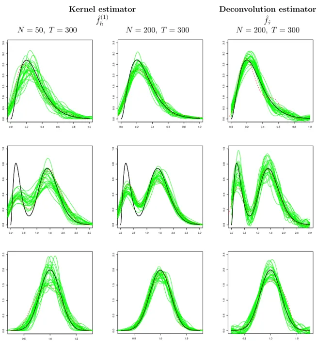
For this model, we use exact simulations for N = 50 and T = 300 or N = 200 and T = 300, withσ = 1,xj = 1. The distributions of the random effects are: Gamma Γ(3, 0.1), where 3 is the shape parameter and 0.1 the scale parameter, mixed gamma 0.3 Γ(3,0.1) + 0.7 Γ(15,0.1), and Gaussian N(1,0.22).
The computation of the kernel estimator is fast as we only need the terminal variableUj(T),
Kernel estimator Deconvolution estimator ˆ fh(1) fˆτˆ N = 50, T = 300 N = 200, T = 300 N = 200, T = 300 0.0 0.2 0.4 0.6 0.8 1.0 0. 0 0. 5 1. 0 1. 5 2. 0 2. 5 3. 0 3. 5 N = 50 , T= 300 0.0 0.2 0.4 0.6 0.8 1.0 0 .0 0 .5 1 .0 1 .5 2 .0 2 .5 3 .0 3 .5 N = 200 , T= 300 0.0 0.2 0.4 0.6 0.8 1.0 0 .0 0 .5 1 .0 1 .5 2 .0 2 .5 3 .0 3 .5 N = 200 , T= 300 0.0 0.5 1.0 1.5 2.0 2.5 3.0 0 .0 0 .2 0. 4 0. 6 0. 8 1. 0 N = 50 , T= 300 0.0 0.5 1.0 1.5 2.0 2.5 3.0 0 .0 0 .2 0 .4 0 .6 0 .8 1 .0 N = 200 , T= 300 0.0 0.5 1.0 1.5 2.0 2.5 3.0 0. 0 0. 2 0. 4 0. 6 0. 8 1. 0 N = 200 , T= 300 0.5 1.0 1.5 0. 0 0. 5 1. 0 1. 5 2. 0 2. 5 N = 50 , T= 300 0.5 1.0 1.5 0 .0 0 .5 1 .0 1 .5 2 .0 2 .5 N = 200 , T= 300 0.5 1.0 1.5 0. 0 0. 5 1. 0 1. 5 2. 0 2. 5 N = 200 , T= 300
Figure 1. Model (1), Geometric Brownian Motion with distribution of the ran-dom effects: Gamma (first line), mixed gamma (second line), and Gaussian (third line). Estimated density for 25 independent samples in thin green: kernel estima-tor (first two columns) and deconvolution estimaestima-tor (last column). True density in bold black. Estimated density for one sample of (φj)’s directly observed with
standard kernel density estimator in bold dotted red.
with a Gaussian kernel. The bandwidthhis selected by cross-validation. The deconvolution-type estimatorfˆτˆis computed, with constantκcalibrated through preliminary simulations toκ= 150.
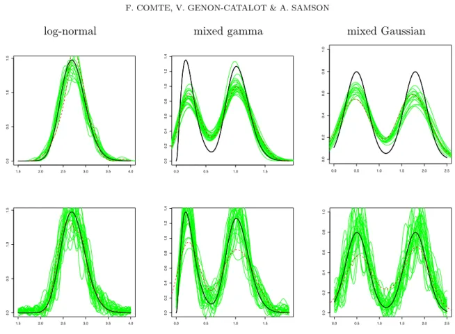
log-normal mixed gamma mixed Gaussian !!"# !$"% !$"# !&"% !&"# !'"% #" # #" % '" # '" % N = 200 , T= 400 !!"# !!"$ !%"# !%"$ !$"# $"$ $ "$ $ "! $ "& $ "' $ "( % "$ N = 200 , T= 400 !!"# !!"$ !%"# !%"$ !$"# $"$ $ "$ $ "! $ "& $ "' $ "( % "$ N = 200 , T= 400
Figure 2. Model (2), multiplicative Ornstein-Uhlenbeck process with distribu-tion of the random effects: log-normal (first column), mixed gamma (second column), and mixed Gaussian (third column). Kernel density estimators (fˆh(1)) for 25 independent samples in thin green. True density in bold black. Estimated density for one sample of (φj)’s directly observed with standard kernel density
estimator in bold dotted red. N = 200, T = 400.
first column gives 25 estimated densities with N = 50, T = 300 for the kernel estimator. In the last two columns, we haveN = 200, T = 300, for the kernel (column 2) and the deconvolu-tion (last column) estimators. Clearly, increasing N improves the result as expected. Note that the methods work well even for T /N not very large. Looking at the last two columns, we see that the deconvolution method seems less biased but with a greater variability than the kernel method. Especially, for a bimodal distribution, the deconvolution methods works well, even bet-ter than when the individual paramebet-ter φj are directly observed (dotted line). Nevertheless, the
deconvolution method is more time consuming as we need to compute all theUj(τ)for1≤τ ≤T.
Model (2). Ornstein-Uhlenbeck process with multiplicative random effect:
(31) dXj(t) =φjXj(t)dt+σdWj(t), Xj(0) =xj.
This model satisfies (H1)-(H2) but not (H4). Nevertheless, it is a classical model. We use the explicit solution: Xj(t) =xjeφjt+σeφjt Z t 0 e−φjsdW j(s).
We use exact simulations of the Xj(kδ) with δ = 0.01, for N = 200 and T = 400, with σ = 1
and xj = 0. The distributions of the opposite of the random effect −φj are: log-normal from normal distributionN(1,0.12), mixed gamma0.3 Γ(3,0.08)+0.7 Γ(15,0.07), and mixed Gaussian
0.5N(0.5,0.252) + 0.5N(1.8,0.252).
To compute the kernel estimator fˆh(1), we replace Uj(T) and Vj(T) by their usual discrete
approximations using discrete data Xj(kδ). The method works well as illustrated by Figure 2 where 25 estimated densities are plotted. Indeed, the graphs are comparable to those obtained from a sample of directly observedφj (bold dotted curves). Again,T /N need not be very large.
Model (3): Ornstein-Uhlenbeck process with additive random effect:
log-normal mixed gamma mixed Gaussian 1.5 2.0 2.5 3.0 3.5 4.0 0. 0 0. 5 1. 0 1. 5 0.0 0.5 1.0 1.5 0. 0 0. 2 0. 4 0. 6 0. 8 1. 0 1. 2 1. 4 0.0 0.5 1.0 1.5 2.0 2.5 0 .0 0 .2 0 .4 0 .6 0 .8 1 .0 N = 200 , T= 400 1.5 2.0 2.5 3.0 3.5 4.0 0 .0 0. 5 1. 0 1. 5 0.0 0.5 1.0 1.5 0 .0 0. 2 0. 4 0. 6 0. 8 1. 0 1. 2 1. 4 0.0 0.5 1.0 1.5 2.0 2.5 0 .0 0. 2 0. 4 0. 6 0. 8 1. 0
Figure 3. Model (3), additive Ornstein-Uhlenbeck process with distribution of the random effects: log-normal (first column), mixed gamma (second column), and mixed Gaussian (third column). Estimated density for 25 independent sam-ples in thin green: kernel estimator (fˆh,δ(4), first line) and deconvolution estimator (f˜τ˜δ,δ, second line). True density in bold black. Estimated density for one sample of(φj)’s directly observed with standard kernel density estimator in bold dotted
red. N = 200, T = 400.
The solution is:
Xj(t) =xje−t+φj(1−e−t) +σe−t Z t 0 esdWj(s). Hence, E(Xj2(t)|φj =ϕ)≤3(xj)2+ϕ2+ σ2 2t.
Provided that Eφ2j < +∞, E(Xj2(t)) ≤ 3((xj)2+Eφ2j +σ2). All assumptions of Section 3 are satisfied. For this model, we use exact simulations of the Xj(kδ) with δ = 1 for N = 200
and T = 400, with σ = 1 and xj = 0. The distributions of the random effects are:
log-normal logN(1, 0.12), mixed gamma 0.4 Γ(3,0.08) + 0.6 Γ(30,0.035), and mixed Gaussian
0.5N(0.5,0.252) + 0.5N(1.8,0.252).
The computation of the kernel estimator fˆh,δ(4) only requires the discretized terminal variable
ˆ
Zj,T while the deconvolution-type estimator f˜˜τδ,δ requires all the variables Zˆj,τ for 1≤τ ≤N
see Proposition 7. The deconvolution-type estimatorf˜τ˜δ,δis computed with constantκ˜calibrated through preliminary simulation experiments to ˜κ= 10.
Figure 3 (25 estimated densities) illustrates the kernel method (first line) and the deconvolution method (second line). The deconvolution method has a great variability but captures well the two modes of the bimodal distributions. On the contrary, the variability band for the kernel estimators is thiner but seems to miss the height of the two modes.
6. Model properties.
In this section, we detail some properties of model (1), give some interpretations of our as-sumptions and look at links between model (2) and (3).
6.1. Existence and uniqueness of strong solutions. We consider N real valued stochastic processes (Xj(t), t ≥ 0), j = 1, . . . , N, with dynamics ruled by (1) where φj are Rd-valued.
Consider the assumptions
(A) The functions (x, ϕ)→b(x, ϕ) and (x, ϕ)→σ(x, ϕ) areC1 on R×Rd, and such that:
∃K >0,∀(x, ϕ)∈R×Rd, |b(x, ϕ)|+|σ(x, ϕ)| ≤K(1 +|x|+|ϕ|).
(B) The functions(x, ϕ)→b(x, ϕ) and (x, ϕ)→σ(x, ϕ) areC1 on R×Rd, and such that:
|b′x(x, ϕ)|+|σx′(x, ϕ)| ≤L(ϕ), |b′ϕ(x, ϕ)|+|σϕ′(x, ϕ)| ≤L(ϕ)(1 +|x|),
withϕ→L(ϕ) continuous.
Under (A) or (B), for allϕ, and allxj ∈R, the stochastic differential equation
(33) d Xjϕ,xj(t) =b(Xjϕ,xj(t), ϕ)dt+σ(Xjϕ,xj(t), ϕ)dWj(t), Xϕ,x
j
j (0) =xj
admits a unique strong solution process (Xjϕ,xj(t), t≥0)adapted to the filtration(Ft, t≥0). LetC(R+,R) be the space of continuous functions onR+, endowed with the Borelσ-field asso-ciated with the topology of uniform convergence on compact sets. The distribution of Xjϕ,xj(.)
is uniquely defined on this space. Now, we can state:
Proposition 8. • Under (A) or (B), for j = 1, . . . , N, equation (1) admits a unique solution process (Xj(t), t ≥ 0), adapted to the filtration (Ft = σ(φj, Wj(s), s ≤ t, j =
1, . . . , N), t ≥ 0) such that the joint process ((Xj(t), φj), t ≥ 0) is Markov and there
exists a measurable functional
(34) (ϕ, x, w.)∈(Rd×R×C(R+,R))→F.(ϕ, x, w.)∈C(R+,R)
such that Xj(.) =F.(φj, xj, Wj(.)).
Given that φi =ϕ, the conditional distribution of (Xj(t), t≥0)is identical to the
distri-bution of the process (Xjϕ,xj(t), t≥0).
The processes (Xj(t), t≥0), j = 1, . . . , N are independent.
• Under (A), if moreover, fork≥1,E(|φi|2k)<∞, then, for all T >0,sup
t∈[0,T]E[Xj(t)]2k<
6.2. Assumption (H4). Let us discuss some implications of Assumption (H4). Under (H4), the function b2/σ2 is non null. If we combine (H4) with the assumption that 0 < σ2
0 ≤ σ2(x) ≤
σ12,∀x∈R, then, we can assume that bothband σ are positive and satisfy:
(H5) (i) 0< c0 ≤b(x)/σ(x)≤c1, (ii) 0< σ0≤σ(x)≤σ1,∀x∈R.
Proposition 9. Let Xi be given by (2),Xj(0) =xj, j= 1, . . . , N under(H5). Then, the process Xi is transient in the sense that:
P( lim
t→+∞Xi(t) = +∞) =P(φi >0), P( limt→+∞Xi(t) =−∞) =P(φi<0).
6.3. Links between the multiplicative and the additive model. In some cases, the mul-tiplicative model can be transformed into an additive model by a change of function.
Proposition 10. Assume that the drift function in model (2) is C1 and satisfies, for some
positive constant b0, b(x)≥ b0 for all x, and set F(x) =R0xdu/b(u). Then the process Yj(t) = F(Xj(t))satisfies dYj(t) = (φj− 1 2 b′◦F−1(Yj(t)) b2◦F−1(Y j(t)) )dt+σ◦F− 1(Y j(t)) b◦F−1(Y j(t)) dWj(t)
The result follows from a standard application of the Itô formula. Consequently, (2) can be treated as (3) after the change of function whenb(·) is lower bounded b y a positive constant.
7. Concluding remarks
In this paper, we consider N i.i.d. processes (Xj(t), t ∈ [0, T]), j = 1, . . . , N, where the
dynamics ofXj is described by a SDE including a random effect φj. The nonparametric density
estimation of φj is investigated in two specific models ((2)-(3)) where the diffusion coefficient does not contain the random effect. The drift term is either multiplicative (b(x, ϕ) =ϕb(x)) or additive (b(x, ϕ) =φ+b(x)). We build kernel and adaptive deconvolution-type estimators and study theirL2-risk as bothNandT =T(N)tend to infinity. Under the theoretical condition that
T(N)/N tends to infinity rather fast, the estimators attain the usual optimal rates. Nevertheless, numerical simulation results on several models show that, in practice,T(N)/N needs not be very large. Extensions of the present work to models with a more general drift are on going work.
8. Proofs 8.1. Proof of Proposition 1. Classically,
E(kf −fˆh(1)k2) = kf −E( ˆfh(1))k2+E(kfˆh(1)−E( ˆfh(1))k2)
≤ 2kf −fhk2+ 2kfh−E( ˆfh(1))k2+E(kfˆh(1)−E( ˆfh(1))k2).
(35)
The last term is the usual variance term and is bounded by (36) E(kfˆh(1)−E( ˆfh(1))k2) = 1 N Z Var(Kh(x−A1,T))dx≤ R K2 N h .
The first term is a usual bias term. The specific term is the middle one. We note thatfh(x) =
E(Kh(x−φ1))and we apply the Taylor Formula with integral remainder:
Kh(x−A1,T)−Kh(x−φ1) = (φ1−A1,T) h2 Z 1 0 K′ 1 h(x−φ1+u(φ1−A1,T)) du
which yields kfh−E( ˆfh(1))k2 = Z (E(Kh(x−A1,T)−Kh(x−φ1)))2dx ≤ Z Eh(Kh(x−A1,T)−Kh(x−φ1))2 i dx = E Z (Kh(x−A1,T)−Kh(x−φ1))2dx ≤ h13 Z (K′)2(y)dyE[(φ1−A1,T)2] = 1 h3 Z (K′)2(y)dyE M1(T) V1(T) 2! ≤ 1 h3 Z (K′)2(y)dy c 2 1 T c4 0 since under (H4), E (M1(T))2 (V1(T))2 ≤ 1 T2c4 0 E[(M1(T))2]≤ 1 T c21 c40.
8.2. Proof of Proposition 2. Since E( ˆfm(2)) =fm, we have
(37) E(kf−fˆm(2)k2) =kf −fmk2+E(kfm−fˆm(2)k2).
Askfm−fˆm(2)k2 = (2π)−1kfm∗ −( ˆf (2)
m )∗k2, and the random vectors (Uj,k)1≤k≤K are independent
and identically distributed forj = 1, . . . , N (see (11)), we get
E(kfm−fˆm(2)k2) = 1 2π Z πm −πmE 1 N K N X j=1 K X k=1 (eiuUj,keu2/∆−E(eiuUj,keu2/(2∆))) 2 du = 1 2πN Z πm −πm Var 1 K K X k=1 eiuU1,keu2/(2∆) ! du = 1 2πN K2 Z πm −πm K X k,k′=1
cov(eiuU1,k, eiuU1,k′)eu2/∆du.
(38)
Looking at (11), we can see that, fork=k′,
cov(eiuU1,k, eiuU1,k′) = 1− |f∗(u)|2e−u2/∆
and for k6=k′,
cov(eiuU1,k, eiuU1,k′) = (1− |f∗(u)|2)e−u2/∆.
Plugging this in (38) yields
(39) E(kfm−fˆm(2)k2)≤ ∆(m) N K + m n where ∆(m) = 1 2π Z πm −πm eu2/∆du.
We now bound∆(m). First ∆(m) = √ ∆ π Z πm/√∆ 0 ev2dv ≤ √ ∆ π e+ Z πm/√∆ 1 ev2dv ! .
Integrating by part and using thatv7→ev2/v2 is nondecreasing forv≥1 imply
Z πm/√∆ 1 ev2dv = " ev2 2v #πm/√ ∆ 1 +1 2 Z πm/√∆ 1 ev2dv v2 ≤ √ ∆ πme π2m2/∆ −2e. Therefore we get ∆(m)≤ √ ∆ π √ ∆ πme π2m2/∆ + e 2 ! . Asf∗ m =f∗1[−πm,πm],kf −fmk2 = (2π)−1 R
|u|≥πm|f∗(u)|2du, which ends the proof of (13) and
thus of Proposition 2. 2
8.3. Proof of Proposition 3. The proof is close to the one of Proposition 2 and simpler. The following decomposition holds:
kfτˆ −fk2 =kfτˆ −fτk2+kfτ −fk2. Then, E(kfˆτ−fτk2) = 1 2πN Z √ τ −√τ
VareiuA1,τeu2/(2τ)du,
where Var(eiuA1,τ) = 1− |f∗(u)|2e−u2/τ. Hence, (40) E(kfˆτ−fτk2) = 1 2πN Z √ τ −√τ (1− |f∗(u)|2e−u2/τ)eu2/τdu≤ √ τ πN Z 1 0 ev2dv.
8.4. Proof of Theorem 1. We have the successive decompositions
kfˆτˆ−fk2 ≤3(kfˆτˆ−fˆˆτ∧τk2+kfˆτˆ∧τ−fˆτk2+kfˆτ−fk2) and kfˆτˆ−fˆτˆ∧τk2 = kfˆτˆ−fˆτk21Iˆτ≥τ = kfˆτˆ−fˆτk2−pen(ˆτ) 1Iˆτ≥τ+ pen(ˆτ)1Iˆτ≥τ ≤ Γˆτ + pen(ˆτ) kfˆτˆ∧τ−fˆτk2 = kfˆτˆ−fˆτk21Iˆτ≤τ = kfˆτˆ−fˆτk2−pen(τ) 1Iˆτ≤τ+ pen(τ)1Iˆτ≤τ ≤ Γˆτˆ+ pen(τ). This yields kfˆτˆ−fk2 ≤ 3(ˆΓτ + pen(ˆτ) + ˆΓˆτ+ pen(τ) +kfˆτ −fk2) ≤ 6(ˆΓτ + pen(τ)) + 3kfˆτ −fk2.
Then, for k≥τ: kfˆk−fˆτk2 ≤ 3(kfˆτ−fτk2+kfˆk−fkk2+kfk−fτk2) Note that kfk−fτk2 = 1 2πkfk∗−fτ∗k 2= 1 2π Z √τ ≤|u|≤√k| f∗(u)|2du ≤ 1 2π Z |u|≥√τ| f∗(u)|2du=kf−fτk2.
Moreover, as the Fourier transforms of fτˆ −fτ andf −fτ have disjoint supports,
kfˆτ−fk2 =kfˆτ −fτk2+kfτ −fk2.
It follows that, for k≥τ:
kfˆk−fˆτk2 ≤3(kfˆk−fkk2+kfˆτ −fk2),
which in turn implies that
ˆ
Γτ ≤3 max
τ≤k≤N2(k
ˆ
fk−fkk2−pen(k)/3) + 3kfτˆ −fk2.
Therefore, gathering inequalities, we get
kfˆτˆ−fk2 ≤18 max τ≤k≤N2(k ˆ fk−fkk2−pen(k)/3) + 6kfˆτ −fk2+ 6pen(τ) and E(kfˆˆτ−fk2) ≤ 18 N2 X k=τ E(kfˆk−fkk2−pen(k)/3) + 6E(kfˆτ −fk2) + 6pen(τ) ≤ 18 N2 X k=τ E(kfˆk−fkk2−pen(k)/3) + 6kfτ−fk2 +61 + R1 0 ev 2 dv π √ τ N + 6pen(τ). Consequently E(kfˆˆτ−fk2)≤6kfτ −fk2+ 6 1 + 1 +R01ev2dv πκ ! pen(τ) + 18 N2 X k=τ E(kfˆk−fkk2− pen(k) 3 ).
Now, we use the Talagrand Inequality to prove the Lemma
Lemma 1. Under the Assumptions of Theorem 1
N2 X k=τ E(kfˆk−fkk2−pen(k)/3)≤ C N.
This and Proposition 3 gives the result of Theorem 1. 2 Proof of Lemma 1. We have that kfˆk −fkk2 = supt∈S√
k,ktk=1|νN(t)| 2 where S m = {t ∈ L2,supp(t∗) = [−m, m]}and νN(t) = 1 2πht ∗,( ˆf k−fk)∗i= 1 2πN N X j=1 Z √ k −√k t∗(−u)(eiuAj,keu2/(2k)−f∗(u))du.
Note that: νN(t) = 1 N N X j=1 (ψt(Aj,k)−E(ψt(Aj,k))) with ψt(x) = 1 2π Z √ k −√k t∗(−u)eiuxeu2/(2k)du.
The class of functions{ψt, t∈S√
k,ktk= 1} is uniformly bounded as follows.
kψtk∞≤ 1 √ 2πktk Z √ k −√k eu2/kdu !1/2 ≤pe/π k1/4 :=M.
By inequality (40), we get that:
E sup t∈S√ k,ktk=1 |νN(t)|2 ! =E(kfˆk−fkk2)≤c √ k/N :=H2, withc=R01ev2
dv/π.At last, let us determine the boundv.
4π2 sup t∈S√ k,ktk=1 Varψt(Aj,k) ≤ sup t∈S√k,ktk=1E ZZ
t∗(u)t∗(−v)ei(u−v)Aj,ke(u2+v2)/(2k)dudv
≤ sup t∈S√ k,ktk=1 ZZ t∗(u)t∗(−v)f∗(u−v)e(u2+v2+(u−v)2)/(2k)dudv ≤ Z √ k −√k Z √ k −√k| f∗(u−v)|2e3(u2+v2)/kdudv !1/2 ≤ 2√ke6 Z 2√k −2√k| f∗(z)|2dz !1/2 ≤ 2√πe3k1/4kfk:= 4π2v
Thus applying the Talagrand Inequality yields with ǫ2 = 1/2that:
E sup t∈S√ k,ktk=1 |νN(t)|2−4H2 ! ≤C1 k1/4 N e −C2k1/4 +k 1/2 N2 e− C3√N ! ,
whereC1, C2, C3 are positive constants. Thus for pen(k)/3 = 4H2, we get
N2 X k=τ E(kfˆk−fkk2−pen(k)/3) = N2 X k=τ E sup t∈S√ k,ktk=1 |νN(t)|2−2H2 ! ≤ CN1 N2 X k=τ k1/4e−C2k1/4 +e−C3k1/4≤ C4 N .
8.5. Proof of Proposition 4. We have
E(kfˆm(3)−fk2) = E(kfˆm(3)−E( ˆfm(3)) +E( ˆfm(3))−fm+fm−fk2)
= kfm−fk2+kE( ˆfm(3))−fmk2+E(kfˆm(3)−E( ˆfm(3))k2)
The term kfm −fk2 = 2π1 R|u|≥πm|f∗(u)|2du is the usual bias term. The additional bias term kE( ˆfm(3))−fmk2 is bounded by kE( ˆfm(3))−fmk2 = 1 2π Z πm −πm| 1 N N X j=1 E(eiuAj,T)−E(eiuφj)|2du = 1 2π Z πm −πm| E(eiuA1,T −eiuφ1)|2du By the Taylor formula,
eiuA1,T −eiuφ1 =eiuφ1
iuM1(T) V1(T)e iuξj,T . Thus kE( ˆfm(3))−fmk2≤ 1 2π Z πm −πm u2E M1(T) V1(T) 2! du Then, under (H4), E (Mj(T))2 (Vj(T))2 ≤ 1 T2c4 0 E[(Mj(T))2]≤ 1 T c2 1 c40. We obtain kE( ˆfm(3))−fmk2 ≤ π 2c2 1 3c4 0 m3 T
Using the Parseval equality, the variance term can be bounded as follows
E(kfˆm(3)−E( ˆfm(3))k2) = 1 2πE Z πm −πm| 1 N N X j=1 (eiuAj,T −E(eiuAj,T))|2du = 1 2π Z πm −πm V ar 1 N N X j=1 eiuAj,T du≤ m N
Finally, we obtain the bound (20). Ifb=σ, E( ˆfm(3)(x)) = 1 2π Z πm −πm e−iuxf∗(u)e−u2/(2T)du.
The risk of the estimator, using repeatedly Parseval equality, is
E(kf−fˆm(3)k2) = kf−fmk2+kfm−E( ˆfm(3))k2+E(kfˆm(3)−E( ˆfm(3))k2) ≤ kf−fmk2+ 1 2π Z πm −πm| f∗(u)|2|e−u2/(2T)−1|2du+ m N ≤ 1 2π Z |u|≥πm| f∗(u)|2du+ 1 8πT2 Z πm −πm| u|4|f∗(u)|2du+m N, (41)
8.6. Proof of Proposition 5. Equations (35) and (36) hold withfˆh(4) instead of fˆh(1) andZ1,T
instead of A1,T. Now we study kfh−E( ˆfh(4))k2, still considering that fh(x) = E(Kh(x−φ1)).
We apply the Taylor Formula with integral remainder:
Kh(x−Z1,T)−Kh(x−φ1) = (φ1−Z1,T) h2 K′ x−φ1 h +(φ1−Z1,T) 2 h3 Z 1 0 (1−u)K” 1 h(x−φ1+u(φ1−Z1,T)) du.
Recall thatφ1 isF0-measurable, thus E((φ1−Z1,T)K′(x−hφ1)) = 0, and we obtain, using
succes-sively the Cauchy Schwarz and the Burkholder-Davis-Gundy inequalities,
kfh−E( ˆfh(4))k2 = Z (E(Kh(x−Z1,T)−Kh(x−φ1)))2dx ≤ Z Eh(Kh(x−Z1,T)−Kh(x−φ1))2 i dx = E Z (Kh(x−Z1,T)−Kh(x−φ1))2dx ≤ 31h5 Z (K”)2(y)dyE RT 0 σ(X1(s))dW(s) 4 T4 ≤ c h5T4kK”k 2E"Z T 0 σ2(X1(s))ds 2# ≤ c h5T2kK”k 2σ4 1.
8.7. Proof of Proposition 6. We know thatexp(Ut−hUit/2)is a martingale ifU is a martingale and E(ehUit/2)<∞. As σ2(x)≤σ2
1 for all x, this implies that
exp iu ∆ Z k∆ (k−1)∆ σ(Xj(s))dW(s) + u2 2∆2 Z k∆ (k−1)∆ σ2(Xj(s))ds !
has conditional expectation 1 given F(k−1)∆. Sinceeiuφj isF(k−1)∆-measurable, we obtain that
E eiuYj,keu 2 2∆2 Rk∆ (k−1)∆σ2(Xj(s))ds = E eiuφjE ei∆u Rk∆ (k−1)∆σ(Xj(s))dW(s)+u 2 2∆2 Rk∆ (k−1)∆σ2(Xj(s))ds|F(k −1)∆ = E(eiuφ1) =f∗(u).
Therefore E( ˆfm(5)(x)) =fm(x)and we decompose the risk in the two usual terms
(42) E(kfˆm(5)−fk2) =kf −fmk2+E(kfˆm(5)−fmk2).
Then we have to compute
E(kfˆm(5)−fmk2) = 1 2πE Z πm −πm 1 N K N X j=1 K X k=1 (eiuYj,keu 2 2∆2 Rk∆ (k−1)∆σ2(Xj(s))ds−f∗(u)) 2 du .
Then using that the terms under expectation are centered, we compute a variance with indepen-dent variables with respect to the index j:
E(kfˆm(5)−fmk2) = 1 2πN Z πm −πmE 1 K K X k=1 (eiuY1,keu 2 2∆2 Rk∆ (k−1)∆σ2(X1(s))ds−f∗(u)) 2 du. Let us denote by Mk = Rk∆ (k−1)∆σ(X1(s))dW(s) and hMik = Rk∆ (k−1)∆σ2(X1(s))ds. Now, for k < ℓ, by conditioning as follows:
coveiu(φ1+Mk)+u2hMik/2, eiu(φ1+Mℓ)+u2hMiℓ/2
= EeiuMk+u2hMik/2E(eiuMℓ+u2hMiℓ/2|F(ℓ
−1)∆)
− |f∗(u)|2
we get that
coveiu(φ1+Mk)+u2hMik/2, eiu(φ1+Mℓ)+u2hMiℓ/2= 1− |f∗(u)|2.
We obtain E(kfˆm(5)−fmk2) = 1 2πN Z πm −πm 1 K2 K X k=1 (eu 2 ∆2 Rk∆ (k−1)∆σ2(X1(s))ds− |f∗(u)|2) +X k6=ℓ (1− |f∗(u)|2) du ≤ 1 2πN K Z πm −πm e u2σ21 ∆2 du+m N.
Gathering the last inequality and (42) gives the result of Proposition 6. 2
8.8. Proof of Theorem 2. The proof follows the steps of Theorem 1. We prove that
E(kf˜τ−fk2)≤ kf−fτk2+ √ τ πN Z 1 0 eσ12v2dv. Then we obtain E(kf˜τ˜−fk2)≤6kfτ −fk2+ 6 1 + 1 +R01eσ21v2dv π˜κ ! g pen(τ) + 18 N2 X k=τ E(kf˜k−fkk2− g pen(k) 3 ).
Then we have to prove
E N2 X k=τ E(kf˜k−fkk2− g pen(k) 3 ) ≤ C′ N.
To this end, we define
˜ νN(t) = 1 N N X j=1 (ψt( ˜Aj,k)−E(ψt( ˜Aj,k))) with A˜j,k = (Zj,k, Z k 0 σ2(Xj(s))ds) and ψt(x, y) = 1 2π Z √ k −√k t∗(−u)eiux+u 2 2k2ydu1I 0≤y≤σ2 1k. We find kψtk∞≤M˜ := q eσ2 1/πk1/4, sup t∈S√ k,ktk=1 |ν˜N(t)|2 ! ≤˜c√k/N := ˜H2
with˜c=R01eσ12v2dv/π. The difference with the proof of Theorem 1 is that, here, we get nothing better than ˜v := NH˜2. This is why we take ǫ2 = 3 log(N)/K
1 in the Talagrand Inequality.
Then, choosingpen(g k)/3≥(1 + 2ǫ2) ˜H2 gives the result and the value of the constantκ˜. 2
8.9. Proof of Proposition 7. For the fisrt point, the proof is very close to the one of Proposition 5. The only difference is that the bias term includes an additional term due to the approximation of Zj,T byZj,Tˆ . We have: Kh(x−Zˆj,T)−Kh(x−Zj,T) = Zj,T −Zj,Tˆ h2 Z 1 0 K′(x−Zj,Tˆ +u(Zj,T −Zj,Tˆ ) h )du.
Using the Cauchy-Schwarz inequality, we get:
Z dxE(Kh(x−Zˆj,T)−Kh(x−Zj,T)) 2 ≤ E(Zj,T −Zˆj,T) 2 h3 Z (K′(y))2dy. It remains to study Zj,T −Zˆj,T = 1 T n X k=1 Z kδ (k−1)δ (b(Xj(s))−b(Xj((k−1)δ)))ds.
Using again the Cauchy-Schwarz inequality and the fact that b is Lipschitz, say with constant
L, yields: E(Zj,T −Zˆj,T)2≤ L2 T n X k=1 Z kδ (k−1)δ (Xj(s)−Xj((k−1)δ))2ds. As Xj(s)−Xj((k−1)δ) = Z s (k−1)δ (φj+b(Xj(u))du+ Z s (k−1)δ σ(Xj(u))dWj(u), we obtain: E(Xj(s)−Xj((k−1)δ))2≤4δ2(Eφ2j+ sup s≥0E [b2(Xj(s))] + 2δσ12.
Thus, E(Zj,T −Zˆj,T)2≤Cδ for some constantC which depends neither on T nor onδ.
Second, we have:
E(kf˜τ,δ −fk2)≤2E(kf˜τ,δ−f˜τk2) + 2E(kf˜τ−fk2).
Thus, we only deal with the additional term:
E(kf˜τ,δ −f˜τk2)≤ 1 2π Z √ τ −√τE| eiuZˆ1,τ+u 2 2τ2 P[τ /δ] k=1 δσ2(X1((k−1)δ))−eiuZ1,τ+u 2 2τ2 Rτ 0 σ2(X1(s)ds|2du.
Forδ <1≤τ, we can prove as above:
E(Z1,τ −Z1,τˆ )2+ 1 τ2E( [τ /δ]X k=1 δσ2(X1((k−1)δ))− Z τ 0 σ2(X1(s))ds)2 ≤Cδ
for some constantC which depends neither onτ nor on δ. Therefore,
E|eiuZˆ1,τ+u 2 2τ2 P[τ /δ] k=1 δσ2(X1((k−1)δ)))−eiuZ1,τ+u 2 2τ2 Rτ 0 σ2(X1(s))ds|2≤Cδ(eu2σ12/τ + u 4 4τ2e 2u2σ2 1/τ), which, integrating with respect tou, gives the result. 2
8.10. Proof of Proposition 8. . Consider the two-dimensional SDE:
dXj(t) = b(Xj(t), φj(t))dt+σ(Xj(t), φj(t))dWi(t), Xj(0) =xj,
dφj(t) = 0, φi(0) =φj.
This clarifies the Markov property of the joint process(Xj(t), φj)once we have proved existence
and unicity of a strong solution. Moreover, the random effectφj thus appears as an unobserved
initial condition.
• Assumption (A) standardly implies that the above two-dimensional SDE admits a unique strong solution and that there exists a functional F such that Xj(.) =F.(φj, xj, Wj(.))
where F. : Rd ×R ×C(R+,R) → C(R+,R) is measurable (see e.g. Karatzas and
Shreve (1997) p.310).
The joint process ((Xj(t), φj(t)≡φj), t≥0)is Markov. By the Markov property, for all
ϕ, xj, the conditional distribution of (Xj(t), φj), t ≥0)given φj =ϕ is the distribution
of
Xjϕ,xj(.) =F.(ϕ, xj, Wj(.)).
As(φj, Wj(.))are independent, the processes(Xj(.))are independent. As(φj, xj) is the
initial condition, the moment result follows.
• Assumption (A) does not cover the case of (2). This is why we also consider (B). Under (B), we proceed in several steps which are classically used to prove regularity w.r.t. an initial condition.
Under (B), for all ϕ, equation (33) admits a unique strong solution. Therefore, there exists a measurable functional
(43) (x, w.)∈R×C(R+,R)→F.(ϕ, x, w.)∈C(R+,R)
such thatXjϕ,xj(.) =F.(ϕ, xj, Wj)is the unique strong solution of (33). Moreover, as the initial condition xj is deterministic, it holds that, for all integer k≥1 and allT >0,
E sup
t∈[0,T]
(Xjϕ,xj(t))2k<+∞.
We now prove that (43) is measurable as a function of (ϕ, x, w.). Step 1
LetH be a compact subset ofRd, we prove that for all xj ∈Rand allT >0,
(44) sup
ϕ∈HE
(sup
u≤T
(Xjϕ,xj(u))2k:=C(T, H)<+∞.
By equation (33), for all ϕ∈H andt≤T,
Xjϕ,xj(t) =xj+ Z t 0 b(Xjϕ,xj(s), ϕ)ds+ Z t 0 σ(Xjϕ,xj(s), ϕ)dWj(s)
By (B), we have, for allϕ,x and k≥1,
b2k(x, ϕ) +σ2k(x, ϕ)≤L(k, ϕ) (1 +x2k),
whereϕ→L(k, ϕ) is continuous. To ease notations, let us set,X(t) =Xjϕ,xj(t), x=xj. We proceed as in Ikeda and Watanabe (1981,Theorem 2.4, p.163). Using the Hölder inequality, the Burholder-Davis-Gundy inequality, we get
Esup u≤t (X(u))2k≤C(k)(x2k+LT(k, ϕ) Z t 0 (1 +Esup u≤s (X(u))2k)ds,
whereC(k) is a constant andϕ→LT(k, ϕ)is continuous. We conclude by the Gronwall
lemma that, for all t≤T,
Esup
u≤t
(X(u))2k≤CT(k, ϕ),
whereϕ→CT(k, ϕ) is continuous. Thus, we get (44).
Step 2
We prove that
(45) ϕ→Xjϕ,xj(.)
is continuous as a functionRd→C(R+,R).
LetH be a compact convex subset ofRd and set, forϕ, ϕ′ ∈H,
St(ϕ, ϕ′) =Esup u≤t Xjϕ,xj(u)−Xjϕ′,xj(u)2k. We have: Xjϕ,xj(t)−Xjϕ′,xj(t) = Z t 0 b(Xjϕ,xj(s), ϕ)−b(Xjϕ′,xj(s), ϕ′)ds + Z t 0 σ(Xjϕ,xj(s), ϕ)−σ(Xjϕ′,xj(s), ϕ′)dWj(s). By (B), we have fors≤T, |b(Xjϕ,xj(s), ϕ)−b(Xjϕ′,xj(s), ϕ′)|+|σ(Xjϕ,xj(s), ϕ)−σ(Xjϕ′,xj(s), ϕ′)| ≤L(ϕ) |Xjϕ,xj(s)−Xjϕ′,xj(s)|+|ϕ−ϕ′|(1 + sup u≤T| Xjϕ′,xj(u)|) !
Now, we proceed as in Step 1. We use the Hölder inequality, the Burkholder-Davis-Gundy inequality, the result (44) of Step 1 and finally the Gronwall lemma to obtain that, for all t≤T,
St(ϕ, ϕ′)≤ |ϕ−ϕ′|2kCT(k, H),
for (another) constant CT(k, H). Now, choosing 2k > d, we can conclude by the
Kol-mogorov continuity of sample paths theorems (see e.g. Revuz and Yor, 1991, Theorem 2.1, p.25), that ωT(δ) = sup ϕ,ϕ′∈H sup t≤T | Xjϕ,xj(t)−Xjϕ′,xj(t)|
tends to 0a.s. asδ tends to0. This gives (45). Step 3
As (43) is measurable for all ϕ, Step 2 standardly implies that
(ϕ, x, w.)∈Rd×R×C(R+,R)→F.(ϕ, x, w.)∈C(R+,R)
is measurable.
The conclusion of Proposition 8 follows.
8.11. Proof of Proposition 9. For the proof, we omit the index j in the notations. Consider a fixed value ϕ >0 and introduce the process Y0(t)given by:
dY0(t) =ϕσ0c0dt+σ(Y0(t))dW(t), Y0(0) =x.
Asϕ > 0,ϕb(x)≥ϕσ0c0 for all x. By the comparison theorem for one-dimensional SDEs (see
e.g. Ikeda and Watanabe 1981, p.352), it holds that Xϕ,x(t)≥Y0(t)for all t≥0. Thus,
Xϕ,x(t) t ≥ x t +ϕσ0c0+ 1 t Z t 0 σ(Y0(s))dW(s) = x t +ϕσ0c0+ Rt 0σ(Y0(s))dW(s) Rt 0σ2(Y0(s))ds Rt 0 σ2(Y0(s))ds t AsR0tσ2(Y0(s))ds≥σ02t, R+∞ 0 σ2(Y0(s))ds= +∞, so Rt 0σ(Y0(s))dW(s) Rt 0 σ2(Y0(s))ds →0, a.s.. As0< Rt 0σ2(Y0(s))ds
t ≤σ12, we deduce that, a.s.,lim inft→+∞X
ϕ,x(t)
t ≥ϕσ0c0, hencelimt→+∞Xϕ,x(t) =
+∞.
Analogously, for ϕ < 0, P(limt→+∞Xϕ,x(t) = −∞) = 1. For ϕ = 0, X0,x(.) is a
martin-gale such that < X0,x >+∞= R0+∞σ(X0,x(s))ds = +∞ a.s.. Hence, P(lim inft→+∞X0,x(t) =
−∞,lim supt→+∞X0,x(t) = +∞) = 1. Noting that
P( lim t→+∞X(t) = +∞|φ=ϕ) =P( limt→+∞X ϕ,x(t) = +∞) = 1 (ϕ>0), we get that P( lim t→+∞X(t) = +∞) =P(φ >0).
The other property follows analogously. 2
8.12. Talagrand Inequality. The following result follows from the Talagrand concentration inequality given in Klein and Rio (2005) and arguments in Birgé and Massart (1998) (see the proof of their Corollary 2 page 354).
Lemma 2. (Talagrand Inequality) LetY1, . . . , Ynbe independent random variables, letνn,Y(ψ) = (1/n)Pni=1[ψ(Yi)−E(ψ(Yi))] and let F be a countable class of uniformly bounded measurable
functions. Then forǫ2 >0
E h sup ψ∈F| νn,Y(ψ)|2−2(1 + 2ǫ2)H2i + ≤ 4 K1 v ne −K1ǫ2nH 2 v + 98M 2 K1n2C2(ǫ2) e− 2K1C(ǫ2)ǫ 7√2 nH M , with C(ǫ2) =√1 +ǫ2−1, K 1= 1/6, and sup ψ∈Fk ψk∞≤M, E h sup ψ∈F| νn,Y(ψ)|i≤H, sup ψ∈F 1 n n X k=1 Var(ψ(Yk))≤v.
By standard density arguments, this result can be extended to the case where F is a unit ball of a linear normed space, after checking that f 7→ νn(ψ) is continuous and F contains a
References
[1] Birgé, L., and Massart, P. (1998) Minimum contrast estimators on sieves: exponential bounds and rates of convergence.Bernoulli4, 329-375.
[2] Comte, F., Rozenholc, Y. and Taupin, M.-L. (2006) Penalized contrast estimator for adaptive density decon-volution.Canadian Journal of Statistics34, 3, 431-452.
[3] Comte, F. and Samson, A. (2012). Nonparametric estimation of random effects densities in linear mixed-effects model,Journal of Nonparametric Statistics,24, 4, 951-975.
[4] Davidian, M., and Giltinan, D.M. (1995). Nonlinear Models for Repeated Measurement Data, New York: Chapman and Hall.
[5] Delattre M., Genon-Catalot V. and Samson A. (2012). Maximum likelihood estimation for stochastic differ-ential equations with random effects.Scandinavian Journal of Statistics, to appear.
[6] Ditlevsen, S. and De Gaetano, A. (2005). Mixed effects in stochastic differential equation models.REVSTAT 3, 137-153.
[7] Donnet, S. and Samson, A. (2008) Parametric inference for mixed models defined by stochastic differential equations.ESAIM Probab. Stat.12, 196-218.
[8] Donnet S, Samson A. (2010). EM algorithm coupled with particle filter for maximum likelihood parameter estimation of stochastic differential mixed-effects models.Preprint MAP5 2010-24.
[9] Goldenshluger, A., Lepski, O. (2011). Bandwidth selection in kernel density estimation: oracle inequalities and adaptive minimax optimality.Ann. Statist.39, 1608-1632.
[10] Ikeda, N. and Watanabe, S. (1989) Stochastic differential equations and diffusion processes. Second edi-tion. North-Holland Mathematical Library, 24. North-Holland Publishing Co., Amsterdam; Kodansha, Ltd., Tokyo.
[11] Karatzas, I. and Shreve, S. (1997).Brownian motion and stochastic calculus. Springer-Verlag, New-York. [12] Klein, T. and Rio, E. (2005). Concentration around the mean for maxima of empirical processes.Ann. Probab.
33, 1060-1077.
[13] Nie, L. (2006) Strong consistency of the maximum likelihood estimator in generalized linear and nonlinear mixed-effects models.Metrika63, 123-143.
[14] Nie, L. (2007). Convergence rate of the mle in generalized linear and nonlinear mixed-effects models: Theory and applications.J. Statist. Plann Inf.137, 1787-1804.
[15] Nie, L. and Yang, M. (2005). Strong consistency of MLE in nonlinear mixed-effects models with large cluster size.Sankhya67, 736-763.
[16] Overgaard, R., Jonsson, N., Tornøe, C. and Madsen, H. (2005). Non-linear mixed effects models with sto-chastic differential equations: Implementation of an estimation algorithm.J. Pharmacokinet. Pharmacodyn. 32, 85-107.
[17] Picchini, U., De Gaetano, A. and Ditlevsen, S. (2010). Stochastic differential mixed-effects models.Scand. J. Statist.37, 67-90.
[18] Picchini, U. and Ditlevsen, S. (2011). Practical estimation of high dimensional stochastic differential mixed-effects models.Comput. Statist. Data Anal.55, 1426-1444.
[19] Pinheiro, J.C. and Bates, D.M. (2000).Mixed-Effects Models in S and S-PLUS. New York, Springer. [20] Revuz, D. and Yor, M. (1999).Continuous martingales and Brownian motion.Third edition. Grundlehren der
Mathematischen Wissenschaften [Fundamental Principles of Mathematical Sciences], 293. Springer-Verlag, Berlin.
[21] Tsybakov, A. B. (2009). Introduction to nonparametric estimation. Revised and extended from the 2004 French original. Translated by Vladimir Zaiats. Springer Series in Statistics. Springer, New York.