Procedia Materials Science 10 ( 2015 ) 446 – 454
2211-8128 © 2015 The Authors. Published by Elsevier Ltd. This is an open access article under the CC BY-NC-ND license (http://creativecommons.org/licenses/by-nc-nd/4.0/).
Peer-review under responsibility of the International Conference on Nanomaterials and Technologies (CNT 2014) doi: 10.1016/j.mspro.2015.06.080
ScienceDirect
* Corresponding author. Tel.: +91-9880994563; fax: +91-80-28437373.
E-mail address: [email protected], [email protected], [email protected]
2nd International Conference on Nanomaterials and Technologies (CNT 2014)
A Novel Approach for Design and Analysis of Diabetic Retinopathy
Glaucoma Detection using Cup to Disk Ration and ANN
P.V.Rao
a*, Gayathri.R
b, Sunitha.R
ca Professor and R&D Head, Department of ECE, Rajarajeswari college of Engineering, Bangalore, India
b Ph.D. Research Scholar, Dept. of ECE, (AIT), Jain University, Bangalore, India c Ph.D Research Scholar, Department of ECE, Rajarajeswari College of Engineering, Bangalore, India
ABSTRACT
Glaucoma is an eye disease which damages the optic nerve of the eye and becomes severe over a period of time. It is caused due to buildup of pressure inside the eye. Glaucoma tends to be inherited and may not show up until later in life. The detection of glaucomatous progression is one of the most important and most challenging aspects of primary open angle glaucoma (OAG) management. It is caused due to buildup of pressure inside the eye. The detection of glaucomatous progression is one of the most important and most challenging aspects of primary open angle glaucoma (OAG) management. The early detection of glaucoma is an important in human life in order to enable appropriate monitoring, treatment and to minimize the risk of irreversible visual field loss. Although advances in ocular imaging offer the potential for earlier diagnosis, the best method is to involve a combination of information from structural and functional tests. In this proposed method both structural and energy features are considered, then analyzed to classify as glaucomatous image. Energy distribution over cup to disk ration were applied to find these important texture energy features. Finally extracted energy features are applied to Multilayer Perceptron (MLP) and Back Propagation (BP) neural network for effective classification by considering normal subject’s extracted energy features. Naive Bayes classifies the images in the database with the accuracy of 89.6%. MLP-BP Artificial Neural Network (ANN) algorithm classifies the images in the database with the accuracy of 90.6%.
Keywords:Z-Score Normalization, Cup-to-Disc, Symlets, Biorthogonal and Daubechies wavelets, MLP-BP ANN
© 2015 The Authors. Published by Elsevier Ltd.
Peer-review under responsibility of the International Conference on Nanomaterials and Technologies (CNT 2014). © 2015 The Authors. Published by Elsevier Ltd. This is an open access article under the CC BY-NC-ND license
(http://creativecommons.org/licenses/by-nc-nd/4.0/).
1.Introduction
Glaucoma is an eye disease which damages the optic nerve of the eye and becomes severe over time. It is caused due to buildup of pressure inside the eye. Glaucoma tends to be inherited and may not show up until later in life. The increased pressure, called intraocular pressure, damages the optic nerve, which transmits pictures to the brain. Glaucoma is an optic neuropathy characterized by distinctive changes in the optic nerve head and visual field [2]. If damage to the optic nerve continues, glaucoma will result in permanent loss of vision [10]. If not medicated, glaucoma can cause total permanent blindness within a few years. People with glaucoma have no early symptoms or pain from this increased pressure. Glaucoma is the second leading cause of blindness in the world. The detection of glaucomatous progression is one of the most important and most challenging aspects of primary open angle glaucoma (OAG) management The early detection of glaucoma is important in order to enable appropriate monitoring and treatment, and to minimize the risk of irreversible visual field loss. Although advances in ocular imaging offer the potential for earlier diagnosis, the best method is to involve a combination of information from structural and functional tests. The systematic and automatic investigation of 2-dim level images is proposed in this paper. Pre-processing should be done in automatic diagnosis of retinal images since the quality of acquired image is usually not good. To improve the quality of retinal image Z Score Normalization is used.
2.Related Work
U. Rajendra Acharya, Automated diagnosis of glaucoma using texture and higher spectra energy features, is proposed higher order spectra (HOS) feature from digital fundus images and SVM for classification with accuracy of 91% [1]. Gwenole quellec proposed classification of glaucoma is normal and abnormal based on false positive and false negative and optimal filter framework for detecting target lesions in retinal images [2]. Linlin Shen and Sen Jia were proposed 3-D Gabor wavelet based approach for pixel-based hyperspectral imagery classification with maximum accuracies of 96.04% and 95.36% [3]. Cheng-Hsuan Li were proposed Spatial–Contextual support vector machine for remote sensed image with overall classification accuracy of the hyperspectral image of the IPS data set with 16 classes is 95.5%. The kappa accuracy is up to 94.9%, and the average accuracy of each class is up to 94.2% [4]. Fereidoun A. Mianji proposed mathematically optimized for unmixing problems with a priori known information ignores some statistical properties of the extracted samples and leads to a suboptimal solution for real situations [5]. Sumeet Dua was proposed wavelet based energy feature for glaucoma classification with accuracy of 93% [6]. N. Annul proposed wavelets, Principal component analysis (PCA) and probabilistic neural network (PNN) with 90% of PCA-PNN and 95% of DWT-PNN [7]. Heidelberg Retina Tomography (HRT) is used for diagnosis of Glaucoma, it is a confocal laser scanning system developed by Heidelberg Engineering. It analyzes 3-dim images of the retina. Thus, any changes in nerve head, called papilla, can be quantitatively characterized [4,11].
3.Problem Statement
Glaucoma that can lead to vision loss very quickly, Glaucoma affects all age groups, including infants, children, and the elderly due to low contrast and noise in images, doctors may have problem to identify the small abnormality conditions in the eye. To address this issue a modified wavelets subbands to extract the energy levels of the glaucoma and MLP-BP ANN algorithms for classification is proposed and analyzed.
4.Methodology
Fig.1. shows the block diagram of proposed method for glaucoma detection. It consists of the following blocks Glaucoma Image Database, Z-Score Normalization, Cup to Disc Ratio, Wavelet processing and ANN Classification.
3
Fig.1. Proposed block diagram of Glaucoma detection
4.1 Glaucoma Image database
The 300 Glaucomaimages of both normal and abnormal eye images are collected from different hospitals of different patients and are stored in database. One of the image is taken from the database and subjected to Glaucoma detection.
4.2 Cup-to-Disc Ratio
The Cup-to-Disc Ratio (CDR) consists of cropped gray optical disc, segmentation and calculation of cup to disc ration. From the given image, it is used to crop the required area of an eye; the selected area is applied for segmentation to segment Glaucoma. CDR is the ratio of the size of the optic cup to the optic disc. It is one of the clinical indicators of glaucoma, and is determined manually by trained ophthalmologists, limiting its potential in mass screening for early detection and is computed as
CDR = VCD VDD Where
VDD= Vertical Disc Diameter.
CDR is an important indicator of glaucoma. The optic cup and disc is first segmented to calculate CDR. To extract the optic disc and cup each retinal fundus image has been captured using a high resolution retinal fundus camera and saved as 3072 x 2048 high resolution digital images.When CDR is greater than a threshold, it is glaucomatous, else healthy eye. Usually for healthy eye the ratio is of 0.2 -0.3. Fig.2 shows the flow chart of CDR algorithm.
Fig.2. Flow chart of Cup to Disc Ratio Algorithm Data base Optic nerve image
Cropped gray optical disc
Segmented optic disc
Bounding box of the disc
Segmented optic cup
Bounding box of the cup
Calculate CDR Glaucoma identified Glaucoma Image Database Cup to Disc Ration Image SegmentationI Wavelet
Processing ClassificationANN Image Pre
4.3 Optic Disc and Optic Cup segmentation
The Optic disc is the entry and exit point for blood vessels for retina. A normal optic disc is orange pink in color. A pale disc is an optic disc which varies in color from a pale pink or orange color to white and is an indication of disease condition. The central depression of variable size in the disc is called the Optic Cup and is usually white in color. In order to extract only this boundary the edge image has to be classified into three groups based on the distance from the center of the optic disc and is achieved by performing K-means clustering to the edge of the image [8]. K-means clustering is a method of cluster analysis which aims to partition n observation into k clusters. Then, the group that contains only edge detection of a disc boundary is selected, and noise can be rejected.
5. Wavelets Processing
Input
Fig.3. DWT two level subbands decomposition
The separable wavelet filters is used to extend 1-D Discrete Wavelet Transform (DWT) to 2-D transform. In separable filters, 1-D transform is applied to all the rows of the input and then is applied to columns resulting in 2-D transform. When one-level 2-D DWT is applied to an image, four transform coefficient sets are created. The four sets are Al, Dh, Dv and Db, where the first letter corresponds to applying either a low pass or high pass filter to the rows, and the second letter refers to the filter applied to the columns. The Two-Dimensional DWT (2D-DWT) converts images from spatial domain to frequency domain. At each level of the wavelet decomposition, each column of an image is first transformed using a 1D vertical analysis filter-bank. The same filter-bank is then applied horizontally to each row of the filtered and sub sampled data. One-level of wavelet decomposition produces four filtered and sub sampled images, known as sub bands [10]. The subbands used in this proposed research work are Daubechies, Biorthogonal, and Symlets, the result of the horizontal 1D-DWT and sub sampling to form a 2D-DWT output image is shown in Fig.3.
A wavelet transform is used as an effective tool in those situations, where one needs multiresolution analysis, providing short windows at high frequencies and long windows at low frequencies [6,7]. Here each image is represented as a p × q gray-scale matrix I[i,j]. The resultant 2-D DWT coefficients are the same irrespective of whether the matrix is traversed from top-to-bottom or bottom-to-top. Hence, there exists four decomposition directions corresponding to 0◦ (horizontal, Dh), 45◦ (diagonal, Dd), 90◦ (vertical, Dv), and 135◦ (diagonal, Dd)
orientations. The decomposition structure for one level is illustrated in Fig.2. In this figure, I is the image, g[n] and
h[n] are the low-pass and high-pass filters, respectively, and A is the approximation coefficient. Where, 2ds1 indicates that rows are down sampled by two and columns by one. 1ds2 indicates that rows are down sampled by one and columns by two. The “×” operator indicates convolution operation. Since the number of elements in these matrices is high, and since it needs only a single number as a representative feature, and employed averaging methods to determine such single valued energy features [2]. These are obtained by the following equations.
ܣݒ݁ݎܽ݃݁ܦ݄1=1×ݍΣΣ|ܦ݄1 (ݔ, ݕ) |ݕ= {ݍ} ݔ= {} --- (1) ܣݒ݁ݎܽ݃݁ܦݒ1=1×ݍΣΣ|ܦݒ1 (ݔ, ݕ) |ݕ= {ݍ} ݔ= {} --- (2) ܧ݊݁ݎ݃ݕ=1/2×ݍ2 (Σ x= {p} Σ y= {q} (ܦݒ1 (ݔ,)) 2 --- (3) Retinal Image A1 Dh Dv Dd Down Sampling Down Sampling Down Sampling Down Sampling Columns X g(n) Columns X h(n) Columns X g(n) Columns X h(n) Rows X g(n) Rows X h(n) Down Sampling Down Sampling
6.ANN Classification
In ANN Classification two architectures are used namely, Multilayer Perceptron and Back Propagation which are described in detail in the following sections:
A multilayer Perceptron is a feed forward artificial neural network algorithm that maps sets of input neurons onto a set computational output [3]. The back propagation is modified version of linear Perceptron in that it uses three or more hidden layers with nonlinear activation function. The back propagation is the most widely applied learning algorithm for multilayer Perceptron in neural networks and it employs gradient descent to minimize the squared error between the network output value and desired output value. Theses error signals are used to calculate the weight updates which represents power of knowledge learnt in the network [7]. Multilayer Perceptron with Back Propagation (MLP-BP) are the main algorithm. Based on the literature survey, MLP-BP algorithm was found to be better than the others in terms of accuracy, speed and performance [9]. The phases involved in ANN are forward phase and backward phase as shown in Fig.4. In back propagation, weights are updated after each pattern and by taking one pattern m at a time as follows:
Fig.4. Multilayer Perceptron Architecture 6.1 Forward Phase
Apply the pattern
X
(lj)to the input layer and propagate the signal forward through the network until the final outputsX
jLhave been calculated for each j and L) 4 ( x s X (lj)w(jl) w(lj) ) 1 L ( D 0 i j ) l ( j ) l ( ¸¸¹ · ¨¨© § T T
¦
Where D (L-1) is the number of neurons in layer (L-1),
X
i(l1)output of the jth neuron in the (l-1) th layer, W ij(i)synaptic weight contained in the current neuron, Wij(i) current neuron’s bias weight, j
l
X
()output of the current neuron.6.2 Backward Phase
In this phase, the weights and biases are updated according to the error gradient-descent vector. After an input vector is applied during the forward computation phase, a network output vector is obtained. A target vector t is
provided to the network, to drive the network’s output toward the expected targeted value [10, 14].
Starting with the output layer, and moving back towards the input layer, calculates the error terms and gradient as follows:
)
5
(
1
L
...
,3
,2
,1
l
for
s
w
L
l
for
u
e
l( 1) j ij ) 1 l( j)l ( x )l ( j°¯
°
®
¦
where
e
lj is the error term for jth neuron in the lthlayer
)
6
(
,...
2
,1
l
for
)
s
(
e
s
()l j ) 1 l( j ) 1 l( jT
where
T
(
s
(lj))
is the derivative if the activation function. Calculate the changes for all the weights as follows:)
7
(
L
,...
2
,1
l
...
x
s
w
l(1) j )l ( j )l ( ijK
'
where K is the learning rate. Update all the weights as follows:
)
8
(
)
L
(
w
)
L
(
w
)
1
L
(
w
(l) ij ) l ( ij ) l ( ij'
Where l=1,2...L (l) and j=0, 1 ...L (l-1), Wij (l)(L) is the current synaptic weight.
Wij (l) (L+1) is the updated synaptic weights to be used in the next feed forward iteration. Fig.4 shows the complete
cycle of period in neural networks training the term period is used to describe a complete pass through all of the training patterns. The weight in the neural net may be updated after each pattern is presented to the net, or they may be updated just once at the end of the period.
7. Implementation and Results
The implementation is done using Matlab 2011b. A Graphical User Interface is created and is as shown in Fig.5. The retinal fundus images are collected from the hospitals and stored in a database. Database consists of fifteen normal retinal images and fifteen glaucomatous retinal images. The image which is to be analysed is selected through the GUI. The selected image is pre-processed using Z-score normalization. The pre-processed image is applied to Wavelet filters Daubechies, Symlets and Biorthogonal. Then feature extraction option is selected to get list of the energy levels extracted from the image. In the GUI, there are two tables: one corresponds to list of energy levels of the input image. The second corresponds to list of selected energy levels of all the images in the database.
7
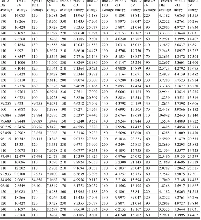
Table 1Enlarged table of the table in the GUI
Table.1 shows the enlarged version of the second table in the GUI. The rows of the table are individual energy level of each retina image in the database. The Columns of the table shows energy level extracted from the images of database with respect to each wavelet filter. First two columns are corresponding to Daubechies filter, the third Db12 Dh1 average Db12 cV energy Sym12 Dh1 average Sym12 cV energy rbio3.7 Dh1 average rbio3.7 cD energy rbio3.7 cV energy rbio3.7 Dh1 average rbio3.9 cD energy rbio3.9 cV energy rbio3.9 cV average rbio4.4 Dh1 average rbio4.4 cH energy rbio4.4 cV energy 150 16.083 150 16.083 260 13.965 41.188 230 9.1801 33.841 220 4.1182 7.6863 31.515 170 18.266 170 18.266 350 15.435 47.205 330 9.9975 39.047 320 5.2522 8.2761 36.286 120 10.428 120 10.428 230 8.5355 25.077 210 5.8071 21.084 190 3.2903 4.9727 19.830 140 9.1697 140 9.1697 270 9.0650 21.893 240 6.2153 18.167 230 3.3333 5.3644 17.031 110 7.6268 110 7.6268 190 6.1105 19.601 170 4.0240 15.707 160 2.2921 3.3995 14.407 130 9.1858 130 9.1858 240 10.047 21.832 220 7.0314 18.032 210 3.2857 6.0837 16.891 110 8.9921 110 8.9921 210 6.8610 24.475 190 4.5708 19.750 170 2.2445 3.8927 18.287 110 8.8547 110 8.8547 200 7.7716 23.148 180 5.1534 18.837 170 2.3693 4.3472 17.594 130 1.1000 130 11.000 230 8.8269 28.980 200 6.1147 23.224 190 2.2607 5.3601 21.400 120 8.1044 120 8.1044 210 7.1364 20.624 200 4.9080 16.889 190 2.5723 4.2792 15.695 100 8.0428 100 8.0428 200 7.5344 20.372 170 5.1164 16.671 160 2.4928 4.4139 15.482 130 9.6110 130 9.6110 280 9.8074 23.305 250 6.7280 19.243 230 3.7208 5.7523 17.914 160 8.7326 160 8.7326 280 8.4659 21.165 250 5.8957 17.474 240 3.3146 5.1627 16.220 120 6.9764 120 6.9764 230 7.3511 17.000 200 5.0603 14.164 190 2.9544 4.3634 13.235 100 8.0723 100 8.0723 190 5.8230 20.309 160 3.8834 16.543 150 1.8239 3.3531 15.319 89.255 9.6231 89.255 9.6231 150 6.6218 25.209 140 4.3798 20.189 130 1.8655 3.7398 18.606 100 8.8988 100 8.8988 190 7.0271 24.269 180 4.6995 19.505 170 2.4418 3.9866 18.152 67.884 9.5880 67.884 9.5880 120 5.5397 24.440 110 3.6764 19.688 110 .96942 3.2443 18.140 79.689 7.9448 79.689 7.9448 150 5.7240 19.558 140 3.9244 15.844 130 1.5574 3.4889 14.722 90.726 6.8426 90.726 6.8426 200 4.6595 17.880 170 2.9594 14.437 160 1.4495 2.4854 13.283 93.858 7.3962 93.858 7.3962 170 5.3136 19.232 150 3.5696 15.600 140 1.6285 3.1009 14.470 96.115 10.342 96.115 10.342 190 9.0772 27.366 170 6.1034 22.223 160 2.5909 5.1879 20.575 120 13.331 120 13.331 230 9.6781 33.990 200 6.2494 27.813 180 2.8689 5.2293 25.862 110 7.6078 110 7.6078 210 6.0777 19.233 190 4.1093 15.753 180 2.1504 3.5577 14.723 97.494 12.479 97.494 12.479 180 10.399 31.826 160 6.9766 26.092 160 2.5486 5.9133 24.379 110 10.096 110 10.096 210 7.8924 26.056 190 5.2300 21.143 180 2.1869 4.4696 19.519 110 12.202 110 12.202 210 9.1694 30.338 190 6.1037 25.047 180 2.8282 5.2042 23.515 92.933 9.0100 92.933 9.0100 180 6.3639 23.396 160 4.1252 18.773 160 2.2542 3.5075 17.301 84.856 7.0662 84.856 7.0662 170 4.9956 19.112 150 3.2166 15.594 140 1.7069 2.7148 14.487 96.40 7.8549 96.401 7.8549 170 6.1773 20.039 160 4.1502 16.195 160 1.8368 3.5917 14.887 150 16.083 150 16.083 260 13.965 41.188 230 9.1801 33.841 220 4.1182 7.6863 31.515 170 18.266 170 18.266 350 15.435 47.205 330 9.9975 39.047 320 5.2522 8.2761 36.286 120 10.428 120 10.428 230 8.5355 25.077 210 5.8071 21.084 190 3.2903 4.9727 19.830 140 9.1697 140 9.1697 270 9.0650 21.893 240 6.2153 18.167 230 3.3333 5.3644 17.031 110 7.6268 110 7.6268 190 6.1105 19.601 170 4.0240 15.707 160 2.2921 3.3995 14.407
and fourth columns are corresponding to symlets12 [4, 5]. The fifth, sixth and seventh columns are corresponding to Biorthogonal filter (Bio3.7). The eighth, ninth and tenth columns are corresponding to Biorthogonal filter (Bio3.9). The eleventh twelve and thirteenth columns are corresponding to Biorthogonal filter (Bio4.4) [8]. Using these energy levels the Naive Bayes and MLP-BP ANN algorithm will classify the images as normal or abnormal [9].
Fig.6 shows the GUI for Wavelets, energy and classification of glaucoma for normal displays the tables corresponding to Naive Bayes and MLP-BP ANN algorithm. Naive Bayes classifies the images in the database with the accuracy of 89.6% MLP-BP ANN algorithm classifies the images in the database with the accuracy of 97.6%. This GUI also shows two popup windows which are nothing but the report generated by Naive Bayes and MLP-BP ANN algorithm for the selected input image. Fig.7 shows the abnormal condition of glaucoma.
Fig.6. Wavelets, energy and classification of glaucoma for normal
Fig.7. Wavelets, energy and classification of glaucoma for abnormal 8.Conclusion and Future Work
For the glaucomatous image, the cup to disc ratio is used to segment glaucoma portion, the segmented image is applied for energy levels extracted using wavelet subbands Daubechies (Db4), Symlets (sym4) and Biorthogonal filters (bio3.7, bio4.2 & bio4.7) gives the clear indication of difference in the energy levels compared to that of normal retina image. The ANN algorithms Naive Bayes and MLP-BP are trained with normal Bayes classifies the images in the database with the accuracy of 89.6%. MLP-BP ANN algorithm classifies the images in the database
with the accuracy of 97.6%. The proposed system exhibits better accuracy compared to existing glaucoma classification systems. This system is cost effective and can be readily used in the hospitals. This system reduces doctor’s burden and overcomes human error. In future the system can be incorporated with artificial intelligence to classify other abnormalities of the eye as well. It can also be designed to generate a report by itself with full information of the patient so that it can be used for telemedicine purpose.
Acknowledgement
We would like to express our sincere thanks to shri. A C Shanmugam, the chairman and Dr. M S Bhagyashekar, the principal, MCET-Rajarajeswari College of Engineering, Bangalore for providing constant support and encouragement during this research work.
References
Annu.N “Classification of Glaucoma Images using Wavelet based Energy Features and PCA”. International Journal of Scientific &
Engineering Research, Volume 4, Issue 5, May-2013 ISSN 2229-5518.
Cheng-Hsuan Li, Bor-Chen Kuo, Member, IEEE, “A Spatial-contextual Support vector machine for remotely sensed image classification”,
IEEE Transanction on Geoscinece and remote sensing, Vol.50,No.3, March 2012, 0196-2892.
Fereidoun A and Mianji, Member, IEEE, “SVM-Based Unmixing-to-Classification Conversion for Hyperspectral Abundance
Quantification”, IEEE Transanction on Geoscinece and remote sensing, Vol.49,No.11, Novenber 2011, 0196-2892.
Gwenole quellec, Stephen R. Russell and Michael D. Abramoff, senior Member, IEEE, “Optimal filter framework for automated, instantaneous detection of lesions in retinal images”, IEEE Transanction on medical imaging, Vol.30, N0.2, February 2011, 0278-0062. Linlin Shen and Sen Jia, “Three-Dimensional gobar wavelets for pixel based hyperspectra imahery classification”, IEEE Transanction on
Geoscinece and remote sensing, Vol.49, N0.12, December 2011, 0196-2892.
Rajendra Acharya.U Sunmeet Due, Xian Du and Chua Kuang, “Automated diagnosis of glaucoma using texture and higher spectra features”, IEEE Transanction on information technology in biomedicine, Vol. 15, No.3, May 2011, 1089-7771.
Shen.L and L. Bai, “Mutualboost learning for selecting Gabor features for face recognition,” Pattern Recognit. Lett., vol. 27, no. 15, pp. 1758–1767, Nov.2006.
Sumeet Dua, Senior Member, IEEE, “Wavelet-based energy features for glaucomatous image classification”, IEEE Transanction on information technology in biomedicine, Vol. 16, No.1, January 2012, 1089-7771.
Tarabalka.Y M. Fauvel, J. Chanussot, and J. A. Benediktsson, “SVM- and MRF-based method for accurate classification of hyperspectral
images,” IEEE Geosci. Remote Sens. Lett., vol. 7, no. 4, pp. 736–740, Oct. 2010.
Yorozu .Y M. Hirano, K. Oka, and Y. Tagawa, “Electron spectroscopy studies on magneto-optical media and plastic substrate interface,”
IEEE Transl. J. Magn. Japan, vol. 2, pp. 740-741, August 1987 [Digests 9th Annual Conf. Magnetics Japan, p. 301, 1982].
Zhao.Y.-Q L. Zhang, and S. G. Kong, “Band-subset-based clustering and fusion for hyperspectral imagery classification,” IEEE Trans. Geosci. Remote Sens., vol. 49, no. 2, pp. 747–756, Feb. 2011.