Electrical energy demand forecasting model development and evaluation with maximum overlap discrete wavelet transform-online sequential extreme learning machines algorithms

energies

Electrical Energy Demand Forecasting Model

Development and Evaluation with Maximum Overlap

Discrete Wavelet Transform-Online Sequential

Extreme Learning Machines Algorithms

1 _{School of Sciences, Institute of Life Sciences and the Environment, University of Southern Queensland,}

Toowoomba, QLD 4350, Australia; [email protected] or [email protected] (M.S.A.-M.); [email protected] (Y.L.)

2 _{Management Technical College, Southern Technical University, Basrah 61001, Iraq} * Correspondence: [email protected]

Received: 7 March 2020; Accepted: 2 May 2020; Published: 6 May 2020

Abstract:To support regional electricity markets, accurate and reliable energy demand (G) forecast models are vital stratagems for stakeholders in this sector. An online sequential extreme learning machine (OS-ELM) model integrated with a maximum overlap discrete wavelet transform (MODWT) algorithm was developed using dailyGdata obtained from three regional campuses (i.e., Toowoomba, Ipswich, and Springfield) at the University of Southern Queensland, Australia. In training the objective and benchmark models, the partial autocorrelation function (PACF) was first employed to select the most significant lagged input variables that captured historical fluctuations in theGtime-series data. To address the challenges of non-stationarities associated with the model development datasets, a MODWT technique was adopted to decompose the potential model inputs into their wavelet and scaling coefficients before executing the OS-ELM model. The MODWT-PACF-OS-ELM (MPOE) performance was tested and compared with the non-wavelet equivalent based on the PACF-OS-ELM (POE) model using a range of statistical metrics, including, but not limited to, the mean absolute percentage error (MAPE%). For all of the three datasets, a significantly greater accuracy was achieved with the MPOE model relative to the POE model resulting in anMAPE=4.31% vs.MAPE=11.31%, respectively, for the case of the Toowoomba dataset, and a similarly high performance for the other two campuses. Therefore, considering the high efficacy of the proposed methodology, the study claims that the OS-ELM model performance can be improved quite significantly by integrating the model with the MODWT algorithm.

Keywords: energy security; time-series forecasting; predictive model for electricity demand; OS-ELM; wavelet transformation; MODWT; sustainable energy management systems

1. Introduction

To promote the application of appropriate strategic measures and provide accurate scheduling of electrical power in energy security platforms, a forecasting model that can reliably and precisely forecast the electricity energy demand (G), is required. Arising from a shift in consumer energy usage, the large fluctuations evident inGdata records leave traditional machine learning models, for example, artificial neural network (ANN) [1], multivariate adaptive regression spline (MARS) [1–3], support vector regression (SVR) [2,3], M5 model tree [3], online sequential extreme learning machine (OS-ELM) [4], and multiple linear regression (MLR) [1] needing to improve their capability to accurately forecast theGdata. To achieve this task, a data pre-processing method, to be implemented before running Energies2020,13, 2307; doi:10.3390/en13092307 www.mdpi.com/journal/energies

Energies2020,13, 2307 2 of 19

the model, is required to address this issue if such data are unsteady, stochastic, or chaotic, as found with real life variables.

Wavelet transformation (WT) algorithm, a popular data pre-processing technique that has been widely adopted in the field of energy forecasting (e.g., [5–10]), has been largely explored to decompose the model input datasets through high and low-pass filters. By applying WT, a more coherent structure of the complex time-series can be supplied and fed to a machine learning model to significantly improve the forecast accuracy. Additionally, energy modelers can potentially address issues of non-stationary input data using the WT algorithm, thereby, assisting the model to be more responsive to the input variables’ stochastic behaviors [5]. Wavelet transformation can also provide the relevant information regarding the time-series decomposition process, including the provision of patterns of energy usage within the time and frequency domains, thereby increasing a forecasting model’s capacity to capture such valuable information at different levels of resolution [7,11]. Because of the detailed information that is produced by WT to convert the data from time domain to frequency domain, a machine learning model can work more intelligently to forecast electricity demand data. The fact that several recent studies have applied the WT algorithm to improve global forecasting accuracies in a range of parameters in several fields, for example, rainfall [11], price of electricity [7,8,10], solar radiation [5,6,9], synthetic hydrological time-series [12], flood levels [13,14], water demand [15], electricity demand [16] and streamflow [17], demonstrates the ability of the WT technique to significantly enhance forecasting accuracy.

Although several research studies (e.g., [5–8,17,18]) have implemented WT for different data forecasting purposes, a recent study in hydrological and water resources forecasting has shown that these studies may have incorrectly applied WT in the data decomposition step. In doing so, they have generated models that should not be employed for real-world forecasting problems because their accuracy is potentially falsely represented [19]. This issue can arise because: (i) future data is drawn upon when the WT uses some data from the testing period to calculate the wavelet and scaling coefficients for the training data, (ii) decomposition levels and wavelet filters are incorrectly selected, and (iii) the training/validation/testing data are split up in an inappropriate manner [19]. It is important to note that these three problems have not been addressed by the current studies in the field of energy forecasting when they apply WT. While some other studies [5,6,17,20,21] have tried to address these issues by applying different forms of WT multiresolution analysis (MRA), for example, discrete wavelet transform (DWT)-MRA or maximal overlap discrete wavelet transform (MODWT)-MRA separately to the training, validation, and testing of data, these approaches require the full time-series to calculate the detail and approximation coefficients, leaving some of the previously mentioned issues unresolved [19]. Therefore, again these studies have failed to apply WT in real-world forecasting problem. Consequently, as only one study has correctly applied MODWT without added MRA to forecast hydrological and water resources, additional studies are needed to explore the impact of MODWT and address the drawbacks cited above when this approach has been used on energy forecasting sector.

In the present study, an OS-ELM model, a fast, reliable and accurate machine learning tool that can offer a better generalization performance than other algorithms in a range of forecasting applications (e.g., regression, classification or time-series) and can learn data one by one as do basic extreme learning machine (ELM) algorithms [22,23], was coupled for the first time with the correct MODWT technique in an effort to forecastGdata. Moreover, OS-ELM input and output parameters as well as weights were randomly and analytically selected, respectively [22]. First, the study selected the significant model input variables using a partial autocorrelation function (PACF) to construct a PACF-OS-ELM (POE) model. The novel MODWT-PACF-OS-ELM (MPOE) model was thus built and compared with the standalone (non-wavelet) POE model to investigate the influence of WT onGforecasting when the MODWT transform was applied separately to each input variable to generate the wavelet and scaling coefficients used in feeding the OS-ELM portion of the model. Data from the three regional campuses (Toowoomba, Ipswich, and Springfield) of the University of Southern Queensland (USQ), Australia, were drawn upon to develop and evaluate the accuracy of these techniques in forecasting dailyG.

Energies2020,13, 2307 3 of 19

To outline how these goals were achieved, this paper is organized as follows. The theory of the OS-ELM and MODWT algorithms are presented in Section2. Section3describes the study area, data, and methods, while model evaluation criteria, results, and discussions are shown in Section4. Finally, the study limitations showing future work opportunities, and conclusions are summarized in Sections5and6, respectively.

2. Theoretical Background

2.1. Online Sequential Extreme Learning Machine Model (OS-ELM)

In this paper, the machine learning data intelligent ELM-based model architecture was employed to design a single-layer feed-forward neural network (SLFN), expressed as [4,24]:

yk= i=M X i=1

ρif(wi.xk+ci) (1)

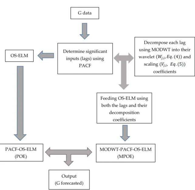
wherek= 1, 2,. . .;N,Mis the hidden nodes ofNinputs (lagged variables generated from partial autocorrelation function (PACF) forGdata or the decomposition of the lagged data resulting from MODWT)xk(t) ={xk}N_k=1∈RN, and output (Gforecasted)yk(x) =yk Nk=1∈Rin the training period). A high-level flowchart is presented in Figure 1to show how these input variables were used to feed the OS-ELM model. f(.) is the activation function, ci ∈ Γ denotes the threshold of theith hidden node, the weight vectors that connect theithhidden node with the input and output nodes are wi= [wi1,wi2,. . .,win]Tandρi= [ρi1,ρi2,. . .,ρim]T, respectively, and the termwi.xkrefers to the inner product ofwiandxi.

According to [24], Equation (1) can be simplified to the form below:

Hρ=Y (2) whereH=             f(w1.x1+c1) · · · f(wM.x1+cM) .. . . .. ... f(w1.xN+c1) · · · f(wM.xN+cM)             0 N×_M

is the hidden layer output matrix of the neural

network,ρ=             ρT 1 .. . ρT M             M×_m andY=             yT₁ .. . yT_N             N×_m .

The following output weight is calculated by applying the least square solution of the linear systems as follows:

ρ=H∗Y (3)

whereH∗denotes the inverse matrix ofH.

With the classical ELM model, allNsamples of data are used during the learning process, making the model relatively time consuming [4]; however, the OS-ELM model, such as the one developed in the present study, addresses this issue: data are only used once within the two learning stages of initialization and sequential learning [4]. The hidden layer output matrix is designed in the initialization step by allocating the input node(wi)and the threshold(ci)to a small piece of initial training data, while the second step of sequential learning is then launched on a one-by-one basis to stop reusing training data [4,22,23,25].

Energies2020,13, 2307 4 of 19

Energies 2020, 13, x FOR PEER REVIEW 4 of 19

𝑊, = ℎ,𝑋 (4)

𝑉, = 𝑔,𝑋 (5)

where 𝑋 is an input time-series vector with 𝑁 values; 𝑗 = 1,2, … 𝐽, where 𝐽 is the decomposition level at the time 𝑖; ℎ, and 𝑔, are the 𝑗th level wavelet (𝑊,) and scaling (𝑉,) filters of MODWT, respectively, and 𝐿 denotes the width of the 𝑗th level filters.

Figure 1. Flowchart showing the model development stages. Figure 1.Flowchart showing the model development stages.

2.2. Maximum Overlap Discrete Wavelet Transform (MODWT)

Serving as a pre-processing method, the MODWT algorithm [26] was implemented before running the model to address non-stationarity issues in time-series datasets by decomposing the input data into high and low-pass filters, resulting in MODWT wavelet and scaling coefficients, respectively (Figure1). Basically, those components are defined as follows [6,19,26]:

Wj,i= l=Lj−1 X l=0 hj,lXi−_1modN (4) Vj,i= l=Lj−1 X l=0 gj,lXi−_1modN (5)

whereXis an input time-series vector withNvalues;j=1, 2,. . .J, whereJis the decomposition level at the timei;hj,landgj,lare thejth level wavelet(Wj,i)and scaling

Vj,i

filters of MODWT, respectively, andLjdenotes the width of thejth level filters.

Energies2020,13, 2307 5 of 19

3. Data and Methods in the Training Period

3.1. Study Area and Data

In the present case study, the ability of the MPOE model to forecast daily electricity demand (G) was tested using electricity use data from three regional university campuses (Toowoomba, Ipswich, and Springfield) of the University of Southern Queensland (USQ), Australia. The historical data were provided by the university campus services for the periods of 1 January 2013 to 31 December 2014 for the main feed of Toowoomba, 1 September 2015 to 31 August 2016 for the main feed and Building A block of Ipswich and Springfield campuses, respectively. Data were recorded every 15-min (96 times per day) in kilowatts (kW), with a total of 70,080 values including 60 zeros for Toowoomba, 35,136 points each for Ipswich and Springfield including 30 zeros and non-zeros, respectively. Zeros were filled in by taking the average values for the points at the same time of day, across the previous month. Daily data were then obtained by summing each set of the 96 values, resulting in 730 points (days) for Toowoomba and 366 points (days) each for Ipswich and Springfield.

Descriptive statistics for the daily time-series datasets are given in Table1, while plots of the series datasets for the three university campuses are shown in Figure2to demonstrate the electricity demand values recorded for each day. The currentGdata clearly showed large fluctuations inGvalues, resulting in the need to implement wavelet transformation through MODWT to address non-stationary issues.

Energies 2020, 13, x FOR PEER REVIEW 5 of 19

3. Data and Methods in the Training Period

3.1. Study Area and Data

In the present case study, the ability of the MPOE model to forecast daily electricity demand (G) was tested using electricity use data from three regional university campuses (Toowoomba, Ipswich, and Springfield) of the University of Southern Queensland (USQ), Australia. The historical data were provided by the university campus services for the periods of 1 January 2013 to 31 December 2014 for the main feed of Toowoomba, 1 September 2015 to 31 August 2016 for the main feed and Building A block of Ipswich and Springfield campuses, respectively. Data were recorded every 15-min (96 times per day) in kilowatts (kW), with a total of 70,080 values including 60 zeros for Toowoomba, 35,136 points each for Ipswich and Springfield including 30 zeros and non-zeros, respectively. Zeros were filled in by taking the average values for the points at the same time of day, across the previous month. Daily data were then obtained by summing each set of the 96 values, resulting in 730 points (days) for Toowoomba and 366 points (days) each for Ipswich and Springfield.

Descriptive statistics for the daily time-series datasets are given in Table 1, while plots of the series datasets for the three university campuses are shown in Figure 2 to demonstrate the electricity demand values recorded for each day. The current G data clearly showed large fluctuations in G

values, resulting in the need to implement wavelet transformation through MODWT to address non-stationary issues.

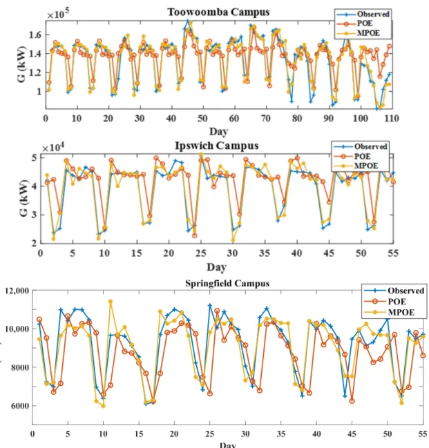
Figure 2. Daily electricity demand (G, kW) time-series for the three study sites of Toowoomba, Ipswich, and Springfield campuses.

Figure 2.Daily electricity demand (G, kW) time-series for the three study sites of Toowoomba, Ipswich, and Springfield campuses.

Energies2020,13, 2307 6 of 19

Table 1.Data splitting and descriptive statistics for theGdata from the University of Southern Queensland campuses’ three stations.

Station Data Period

(dd-mm-yyyy)

Original 15-Mins Data No. Daily Data Points Descriptive Statistics for the Whole Daily Datasets

Total No. Zeros Total Training (70%) Validation (15%) Testing (15%) Minimum (kW) Maximum (kW) Mean (kW)

Toowoomba campus (Main feed) 01-01-2013 to 31-12-2014 70,080 60 730 512 109 109 81,579.70 195,037 141,328 Ipswich campus (Main feed) 01-09-2015 to 31-08-2016 35,136 30 366 256 55 55 23,336 62,378.06 43,716.96 Springfield campus (A Block) 35,136 0 5214 13,536.80 8310.05

Energies2020,13, 2307 7 of 19

3.2. Forecast Model Development and Validation

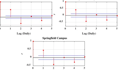
In this study, the proposed MPOE model and its traditional non-WT equivalent POE were developed under the MATLAB environment running on an Intel i7 processor at 3.60 GHz. The original (non-wavelet) dataset with its statistically significant lagged variables, identified using the partial autocorrelation function (PACF) operating in a 95% confidence interval, was used as an input to develop the classical POE model. Figure3illustrates the number of those lags used to build the model where the first two significant lags were selected using the data from all three study sites.

Energies2020, 13, 2307 7 of 19

3.2. Forecast Model Development and Validation

In this study, the proposed MPOE model and its traditional non-WT equivalent POE were developed under the MATLAB environment running on an Intel i7 processor at 3.60 GHz. The original (non-wavelet) dataset with its statistically significant lagged variables, identified using the partial autocorrelation function (PACF) operating in a 95% confidence interval, was used as an input to develop the classical POE model. Figure 3 illustrates the number of those lags used to build the model where the first two significant lags were selected using the data from all three study sites.

Figure 3. The model input variables constructed from the statistically significant lags at a 95%

confidence interval from the original daily G-datasets in the training period for the three study sites

based on correlation coefficient (r) of predictors (lags) using the partial autocorrelation function

(PACF).

On the other hand, to construct the MPOE model, wavelet transformation through MODWT was employed on the individual PACF lagged variables, and the wavelet outputs (wavelet and scaling coefficients) were used along with the PACF lagged components as model inputs. The critical task in achieving a robust model with wavelet transformation is to identify the type of wavelet scaling (ℎ𝑗𝑗,𝑙𝑙/𝑔𝑔𝑗𝑗,𝑙𝑙) filter and the decomposition level (𝐽𝐽). As no single technique to select the best filter and the level of decomposition can be confirmed in the literature [6,27], a trial-and-error method was employed in the present case. Defining a total of 30 wavelet filters, four different widely tested wavelet families (e.g., [5,6,12,17,19]) were used: Daubechies (𝑑𝑑𝑑𝑑𝑖𝑖,𝑖𝑖= 1,2,⋯,10), where 𝑑𝑑𝑑𝑑1 is the same as the Haar wavelet (haar); Fejer–Korovkin (𝑓𝑓𝑘𝑘𝑖𝑖,𝑖𝑖= 4,6,8,14,18,22); Coiflets (𝑐𝑐𝑐𝑐𝑖𝑖𝑓𝑓𝑖𝑖,𝑖𝑖= 1,2,⋯,5); and Symlets (𝑠𝑠𝑦𝑦𝑠𝑠𝑖𝑖,𝑖𝑖= 2,3,⋯,10). The maximum level of decomposition (𝐽𝐽) was computed using Equation (6) [6,17,28]:

𝐽𝐽=𝑖𝑖𝑖𝑖𝑡𝑡(log2𝑁𝑁) (6)

where 𝑁𝑁 is the number of daily data points in this work, and 𝑖𝑖𝑖𝑖𝑡𝑡() is the function that returns the nearest integer. For example, for the Toowoomba campus data, a value of 𝐽𝐽 = 9 was computed, so all possible levels of decomposition (𝐽𝐽= 1,2, … 9) were tested. More details about the MODWT filter and the decomposition level are shown in Table 2. Figure 4 shows the two MODWT wavelet coefficients (WC1 and WC2) and the MODWT scaling coefficient (SC) using lag 1 data from the Toowoomba campus with the best wavelet filter (𝑓𝑓𝑘𝑘8) and decomposition level (2). The results of MODWT (wavelet and scaling coefficients) with 𝑑𝑑𝑑𝑑2 and 𝑑𝑑𝑑𝑑3 were found to be the same as those with 𝑠𝑠𝑦𝑦𝑠𝑠2 and 𝑠𝑠𝑦𝑦𝑠𝑠3, for all study datasets, respectively.

While forecasting models must go through training, validation, and testing datasets, there is no single agreed-upon scenario for data splitting [2,3,5]. Accordingly, these data were divided into

0 1 2 3 4 5 Lag (Daily) -0.5 0 0.5 1 r Toowoomba Campus 0 1 2 3 4 5 Lag (Daily) -0.5 0 0.5 1 r Ipswich Campus 0 1 2 3 4 5 Lag (Daily) -0.5 0 0.5 1 r Springfield Campus

Figure 3.The model input variables constructed from the statistically significant lags at a 95% confidence interval from the original dailyG-datasets in the training period for the three study sites based on correlation coefficient (r) of predictors (lags) using the partial autocorrelation function (PACF).

On the other hand, to construct the MPOE model, wavelet transformation through MODWT was employed on the individual PACF lagged variables, and the wavelet outputs (wavelet and scaling coefficients) were used along with the PACF lagged components as model inputs. The critical task in achieving a robust model with wavelet transformation is to identify the type of wavelet scaling (hj,l/gj,l)filter and the decomposition level(J). As no single technique to select the best filter and the level of decomposition can be confirmed in the literature [6,27], a trial-and-error method was employed in the present case. Defining a total of 30 wavelet filters, four different widely tested wavelet families (e.g., [5,6,12,17,19]) were used: Daubechies (dbi, i=1, 2,· · · , 10), wheredb1is the same as the Haar wavelet (haar); Fejer–Korovkin (f ki, i=4, 6, 8, 14, 18, 22); Coiflets (coi fi,i=1, 2,· · ·, 5);. and Symlets(symi, i=2, 3,· · ·, 10). The maximum level of decomposition(J)was computed using Equation (6) [6,17,28]:

J=intlog₂N (6)

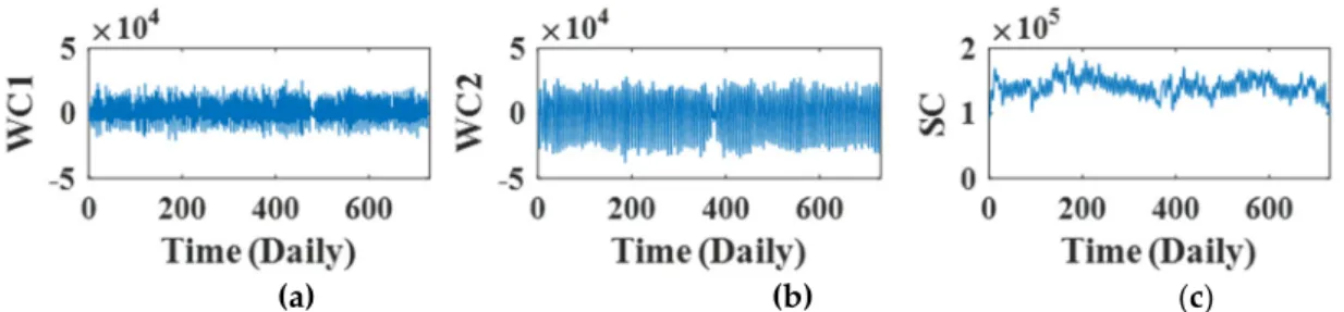
whereNis the number of daily data points in this work, andint(). is the function that returns the nearest integer. For example, for the Toowoomba campus data, a value ofJ.=9 was computed, so all possible levels of decomposition(J=1, 2,. . .9)were tested. More details about the MODWT filter and the decomposition level are shown in Table2. Figure4shows the two MODWT wavelet coefficients (WC1 and WC2) and the MODWT scaling coefficient (SC) using lag 1 data from the Toowoomba campus with the best wavelet filter (f k8) and decomposition level (2). The results of MODWT (wavelet and scaling coefficients) withdb2. anddb3were found to be the same as those withsym2andsym3, for all study datasets, respectively.

Energies2020,13, 2307 8 of 19

Table 2.Optimum model performance and parameters in the training and validation phases based on correlation coefficient (r) and root-mean square error (RMSE; kW), for the three stations with the daily forecast horizon. The models inboldfaceare the optimal (best performing) models.

Station Model No. Hidden

Neurons

No. Wavelet/Scaling Filter No. Wavelet Level No. Models Developed Best Model Training Validation Wavelet/Scaling

Filter Wavelet Level

Hidden Neuron Size r RMSE (kW) r RMSE (kW) Toowoomba

campus (Main feed)

POE 100 Non-wavelet model 100 0.70 17715.42 0.74 16284.72 Non-wavelet model 9

MPOE 100 30 9 27,000 0.96 7260.42 0.94 8026.74 fk8 2 90

Ipswich campus (Main feed)

POE 100 Non-wavelet model 100 0.68 6944.43 0.67 7543.30 Non-wavelet model 10

MPOE 100 30 8 24,000 0.97 2476.19 0.90 4279.08 db2/sym2 3 54

Springfield campus (A Block)

POE 100 Non-wavelet model 100 0.65 1036.28 0.61 1641.08 Non-wavelet model 4

Energies2020,13, 2307 9 of 19

Energies 2020, 13, x FOR PEER REVIEW 8 of 19

70:15:15 for training: validation: testing (Table 1). Data normalization, a very common practice in machine learning, was applied using Equation (7) to scale values down to a range of (0 1), thereby avoiding large numbers in the predictor values of datasets [29]. De-normalization was then applied on predicted data to scale those data back to their original range before models were evaluated.

𝑥 = 𝑥 − 𝑥

𝑥 − 𝑥 (7)

The MATLAB-based OS-ELM function [23], was used to build the present OS-ELM models in this paper. The most important step in developing an OS-ELM model is the selection of the activation function (𝑓(. )) and the hidden neuron size (𝑀; Equation (1)). The radial basis function (RBF) was employed as the activation function in developing the present model, while values of hidden neuron size from 1 to 100 were tested, resulting in 100 POE models for each of the three stations. Additionally, many MPOE models were developed as a result of the numbers of hidden neuron size (𝑀), wavelet filters and decomposition levels (𝐽); for example 100 (𝑀) × 30 (wavelet filters) × 9(𝐽) = 27000 models for the Toowoomba site alone. Table 2 summarizes the details of model development including those factors tested in the training period.

The model accuracy statistics of Pearson correlation coefficient (r) and root-mean square error (RMSE; kW) were used to assess the performance of the POE and MPOE models in the training and validation periods, and thereby to identify the best wavelet and model parameters (Table 2).

𝑟 = ∑ 𝐺 − 𝐺 (𝐺 − 𝐺 )

∑ 𝐺 − 𝐺 ∙ ∑ 𝐺 − 𝐺 (8)

𝑅𝑀𝑆𝐸 = 1

𝑛 𝐺 − 𝐺 (9)

where n is the total number of values of forecast (or observed) G, 𝐺 and 𝐺 are the ith _forecasted

and observed values, while 𝐺 and 𝐺 are the means of the forecasted and observed values, respectively, in the training period.

The statistical metrics of r and RMSE indicate the greatest model accuracy when they approach 1 and 0, respectively. For all the three sites, MPOE models outperformed POE models. For example, for the Toowoomba campus, the MPOE training/validation model accuracy statistics were r = 0.96/0.94 and RMSE = 7260.42/8026.74 kW with 𝑓𝑘 , 2 and 90 as the best wavelet filter, decomposition level, and hidden neuron size, respectively. Comparatively, the POE training/validation model accuracy was poorer: r = 0.70/0.74 and RMSE = 17,715.42/16,284.72 kW for the best hidden neuron size of 9.

(a) (b) (c)

Figure 4. Maximum overlap discrete wavelet transform (MODWT) coefficients constructed using lag 1 of the Toowoomba campus dataset with the optimum wavelet (scaling) filter (𝑓𝑘 ) and wavelet level 2. WC (a, b) and SC (c) represent the wavelet and scaling coefficients, respectively.

Figure 4.Maximum overlap discrete wavelet transform (MODWT) coefficients constructed using lag 1

of the Toowoomba campus dataset with the optimum wavelet (scaling) filter(f k8)and wavelet level 2.

WC (a, b) and SC (c) represent the wavelet and scaling coefficients, respectively.

While forecasting models must go through training, validation, and testing datasets, there is no single agreed-upon scenario for data splitting [2,3,5]. Accordingly, these data were divided into 70:15:15 for training: validation: testing (Table1). Data normalization, a very common practice in machine learning, was applied using Equation (7) to scale values down to a range of(0 1), thereby avoiding large numbers in the predictor values of datasets [29]. De-normalization was then applied on predicted data to scale those data back to their original range before models were evaluated.

xnormalized=

x−_xminimum

xmaximum−xminimum (7)

The MATLAB-based OS-ELM function [23], was used to build the present OS-ELM models in this paper. The most important step in developing an OS-ELM model is the selection of the activation function(f(.))and the hidden neuron size(M; Equation (1)). The radial basis function (RBF) was employed as the activation function in developing the present model, while values of hidden neuron size from 1 to 100 were tested, resulting in 100 POE models for each of the three stations. Additionally, many MPOE models were developed as a result of the numbers of hidden neuron size(M), wavelet filters and decomposition levels(J); for example 100(M)×_{30 (wavelet} filters)×_{9(J) =27000 models for the Toowoomba site alone. Table2summarizes the details of model} development including those factors tested in the training period.

The model accuracy statistics of Pearson correlation coefficient (r) and root-mean square error (RMSE; kW) were used to assess the performance of the POE and MPOE models in the training and validation periods, and thereby to identify the best wavelet and model parameters (Table2).

r= Pi=n i=1 Gobs i −Gobs G_if or−_Gf or r Pi=n i=1 Gobs i −Gobs 2 · r Pi=n i=1 G_if or−_Gf or2 (8) RMSE= v u t 1 n i=n X i=1 G_if or−_Gobs i 2 (9)

wherenis the total number of values of forecast (or observed)G,G_if orandGobs_i are theith forecasted and observed values, whileGf orandGobs_{are the means of the forecasted and observed values, respectively,} in the training period.

The statistical metrics ofrandRMSEindicate the greatest model accuracy when they approach 1 and 0, respectively. For all the three sites, MPOE models outperformed POE models. For example, for the Toowoomba campus, the MPOE training/validation model accuracy statistics werer=0.96/0.94 andRMSE=7260.42/8026.74 kW with f k8, 2 and 90 as the best wavelet filter, decomposition level, and hidden neuron size, respectively. Comparatively, the POE training/validation model accuracy was poorer:r=0.70/0.74 andRMSE=17,715.42/16,284.72 kW for the best hidden neuron size of 9.

Energies2020,13, 2307 10 of 19

4. Model Evaluation and Results in the Testing Period

4.1. Model Prediction Quality

As the quality of model forecasts ofGdata cannot be established by a single statistical metric for the testing phase [30], additional measures, besides theRMSE(Equation (9)), were used [30–39]. These included the Mean absolute error (MAE), relative root-mean square error (RRMSE%), and relative mean absolute error (MAPE%),

MAE= 1 n i=n X i=1 G f or i −G obs i (10) RRMSE=100× r 1 nPii==n1 G_if or−_Gobs i 2 Gobs (11) MAPE=100×1 n i=n X i=1 G_if or−_Gobs i Gobs_i (12) ThisMAEshows the model approaching perfection as its value approaches 0. TheRRMSEand MAPE, both best when approaching 0, present an assessment of model accuracy relative to the range and mean of the forecasted parameter, when a clear evaluation cannot be provided by theRMSEor MAEalone [17]. Model performance is considered to be excellent whenRRMSE<10%, good if 10%< RRMSE<20%, fair if 20%<RRMSE<30%, and poor ifRRMSE>30% [9,31,40,41].

Further model accuracy indexes include the Willmott’s Index (WI), Nash–Sutcliffe model efficiency coefficient (ENS) and Legates and McCabe’s Index (LM) below where values closest to 1 indicate the best performance. WI=1−              Pi=n i=1 G_if or−_Gobs i 2 Pi=n i=1 G f or i −Gobs + G obs i −Gobs 2              , and 0≤_WI≤_{1 (13)} ENS=1−              Pi=n i=1 G_if or−_Gobs i 2 Pi=n i=1 Gobs_i −_Gobs2              , and∞ ≤_ENS ≤_{1 (14)} LM=1−          Pi=n i=1 G obs i −G f or i Pi=n i=1 G obs i −Gobs          , and(∞ ≤_ELM≤_{1) (15)}

Two statistical tests were also used to show that the MPOE model performs better than the POE model. Those were Wilcoxon Signed-Rank test [42–44] andTtest [2]. They were performed with 0.05 significance level and 2-tailed hypothesis.

4.2. Results and Discussion

Using a plethora of model accuracy statistics (i.e., Equations (9)–(15)), the capability and accuracy of the MPOE model in forecasting daily electricity demand (G) was evaluated and compared to that of a traditional POE model, both drawing on testing datasets obtained from three USQ campuses (Toowoomba, Ipswich, and Springfield). While several models were developed and evaluated in this study, only results from optimum models, selected from these several trained models, are shown in Table3. For all three stations’ datasets, the MPOE model showed close to 50% lower values ofRMSE,

Energies2020,13, 2307 11 of 19

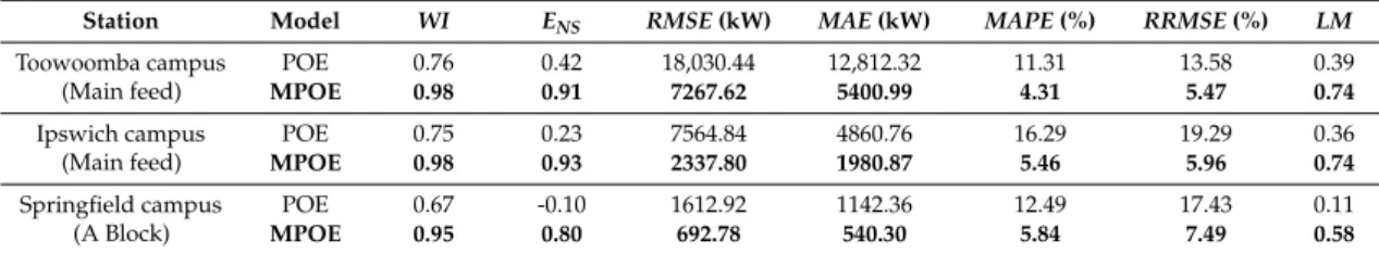
MAE, RRMSEandMAPEand near 50% greater values ofENSandLMthan those of the POE model. For example, for the Toowoomba campus dataset, the MPOE model (MAPE=4.31%,LM=0.74) clearly outperformed the POE model (MAPE=11.31%,LM=0.39). Moreover, the MPOE model yielded better WIvalues (0.98, 0.98, and 0.95) than the POE model (0.76, 0.75, and 0.67) for the Toowoomba, Ipswich, and Springfield study areas, respectively. This comparison (Table3) demonstrated the MPOE model to have yielded a better performance than the non-wavelet POE model.

Table 3.Optimum model performance in the testing phase for daily forecast horizon based on Willmott’s Index (WI), Nash–Sutcliffe model efficiency coefficient (ENS), root-mean square error (RMSE; kW), mean absolute error (MAE; kW), mean absolute percentage error (MAPE%), relative root-mean square error (RRMSE%), as well as Legates and McCabes Index (LM) for the three stations. The models in

boldfaceare the optimal (best performing) models.

Station Model WI ENS RMSE(kW) MAE(kW) MAPE(%) RRMSE(%) LM

Toowoomba campus (Main feed) POE 0.76 0.42 18,030.44 12,812.32 11.31 13.58 0.39 MPOE 0.98 0.91 7267.62 5400.99 4.31 5.47 0.74 Ipswich campus (Main feed) POE 0.75 0.23 7564.84 4860.76 16.29 19.29 0.36 MPOE 0.98 0.93 2337.80 1980.87 5.46 5.96 0.74 Springfield campus (A Block) POE 0.67 -0.10 1612.92 1142.36 12.49 17.43 0.11 MPOE 0.95 0.80 692.78 540.30 5.84 7.49 0.58

Additionally, to ensure the superiority of the proposed approach and support the results introduced in Table3, Wilcoxon Signed-Rank test andTtest have been presented in Table4for the forecasted error statistic|_FE| ₌ G f or i −Gobsi

generated by the MPOE model against the

|_FE|_{generated by the} POE model. With 0.05 significance level and 2-tailed hypothesis, significant results were shown in both tests (pvalue<0.05). These results clearly indicate that the MOPE model receives the significance than the POE model.

Table 4.Wilcoxon Signed-Rank test andTtest results for the|FE|_{of the MOPE model vs. the}|FE|_for the POE model.

Station Wilcoxon Signed-Rank Test TTest pValue pValue

Toowoomba campus (Main feed) 0.00001 0.00001

Ipswich campus (Main feed) 0.00076 0.00053

Springfield campus (A Block) 0.00018 0.00043

To further examine the success of the MPOE model over the POE model forGforecasting in the testing period, observed and forecasted values were plotted as ordinate and abscissa for each model (Figures5and6), and models’ absolute forecasted errors|FE|(Figure7). Time-series plots in Figure5show that the wavelet models have achieved greater accuracy (closer to observed) than the wavelet-free models for all sites.

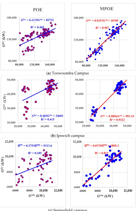
Scatterplots (Figure6) show the coefficient of determinationR2

and the linear regression line (Gf or = aGobs+bwhereais the slope and bis the ordinate intercept) between the observed and forecasted values. The greaterR2_{and values ofaandbcloser to 1 and 0, respectively, showed that} the MPOE model outperformed the POE model when using each of the campus datasets. For the Ipswich campus dataset, the MPOE model yieldedR2=0.93, a=0.99 andb=993.15, in contrast to R2=0.42, a=0.47 andb=24601 for the POE model.

Energies2020,13, 2307 12 of 19

Energies 2020, 13, x FOR PEER REVIEW 12 of 19

Figure 5. Observed vs. forecasted G data in the testing period with the optimal POE and MPOE models for the three study sites.

Scatterplots (Figure 6) show the coefficient of determination (𝑅 ) and the linear regression line (𝐺 = 𝑎𝐺 + 𝑏 where 𝑎 is the slope and 𝑏 is the ordinate intercept) between the observed and forecasted values. The greater 𝑅 and values of 𝑎 and 𝑏 closer to 1 and 0, respectively, showed that the MPOE model outperformed the POE model when using each of the campus datasets. For the Ipswich campus dataset, the MPOE model yielded 𝑅 = 0.93, 𝑎 = 0.99 and 𝑏 = 993.15, in contrast to

𝑅 = 0.42, 𝑎 = 0.47 and 𝑏 = 24601 for the POE model.

Figure 5.Observed vs. forecastedGdata in the testing period with the optimal POE and MPOE models for the three study sites.

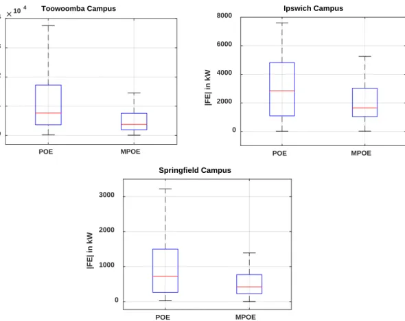
Using boxplots (Figure7) and all station datasets, the MPOE and POE models were compared based on their 25%, 50% and 75% quartiles (lower, middle, upper line of box) as well as maximum and minimum values of the forecasted error statistic|_FE|₌

G f or i −G obs i

. Consequently, the statistical error criteria generated for the MPOE model were significantly lower than those for POE.

Overall, from the results in Tables3and4, as well as Figures5–7, we can conclude that the MPOE model has achieved better forecasting performance than the POE model by generating lower values from MAE, MAPE%, RMSE, and RRMSE% (Table3), larger values from WI, ENS and LM (Table3), significant p values (Table4), closer forecasted values to the observed values (Figure5), better values fromR2_{, aandb(Figure6) and lower|FE|(Figure7). The reason behind this is that the MODWT} method has successfully addressed the non-stationarity issues in time-series datasets before running the POE model to enhance the forecasting accuracy.

Energies2020,13, 2307 13 of 19

Energies 2020, 13, x FOR PEER REVIEW 13 of 19

(a) Toowoomba Campus

(b) Ipswich campus

(c) Springfield campus

Figure 6. Scatterplots of the observed and forecasted G data in the testing phase with the optimal models of POE and MPOE. Equations of linear regression and the coefficient of determination are incorporated. (a) Toowoomba Campus. (b) Ipswich campus. (c) Springfield campus.

Using boxplots (Figure 7) and all station datasets, the MPOE and POE models were compared based on their 25%, 50% and 75% quartiles (lower, middle, upper line of box) as well as maximum and minimum values of the forecasted error statistic |𝐹𝐸| = |𝐺 − 𝐺 |. Consequently, the statistical error criteria generated for the MPOE model were significantly lower than those for POE.

Gfor_{= 0.4139G}obs_{+ 82732} R² = 0.469 80,000 130,000 180,000 80,000 120,000 160,000 G for (kW)

POE

MPOE

Figure 6. Scatterplots of the observed and forecastedGdata in the testing phase with the optimal models of POE and MPOE. Equations of linear regression and the coefficient of determination are incorporated. (a) Toowoomba Campus. (b) Ipswich campus. (c) Springfield campus.

Energies2020,13, 2307 14 of 19

Energies2020, 13, 2307 14 of 19

Figure 7. Boxplots of the absolute forecasted error |FE| in the testing dataset for the three study sites with the optimal models of POE and MPOE.

Overall, from the results in Tables 3 and 4, as well as Figures 5–7, we can conclude that the MPOE model has achieved better forecasting performance than the POE model by generating lower values from MAE, MAPE%, RMSE, and RRMSE% (Table 3), larger values from WI, ENS and LM (Table 3), significant p values (Table 4), closer forecasted values to the observed values (Figure 5), better values from 𝑅𝑅2_{,𝑎𝑎 and 𝑑𝑑 (Figure 6) and lower |FE| (Figure 7). The reason behind this is that the MODWT}

method has successfully addressed the non-stationarity issues in time-series datasets before running the POE model to enhance the forecasting accuracy.

5. Challenges and Future Work

While this study was the first to apply the best suitable wavelet transforms to energy forecasting datasets, thereby achieving a high performance MPOE model, some limitations should be addressed in upcoming works, in particular, the incorporation of external datasets, such as climate variables, which can be downloaded from different sources (e.g., SILO [45], the European Centre for Medium Range Weather Forecasts (ECMWF) and global numerical weather prediction models [1,46] and NASA’s Moderate Resolution Imaging Spectroradiometer (MODIS) [47–50]). These can be decomposed together with lag values using MODWT. The OS-ELM model will be then fed by the wavelet and scaling components resulting from the climate and lag variables, to develop a very high-dimensional model. Although this study has used a good amount of data (730 days and 366 days), a larger power grid model should be built and evaluated using larger datasets from electricity demand (G) to support national electricity markets. This could be achieved by testing the proposed method of this work with a larger study area or incorporating new datasets from the University of Southern Queensland (study area) when these data are available. However, given the large number of input variables that would be generated by MODWT, a method to select and narrow down the best input variables or a very fast model would be necessary to speed up the development step. Accordingly,

POE MPOE 0 1 2 3 4 |FE| in kW 104 Toowoomba Campus POE MPOE 0 2000 4000 6000 8000 |FE| in kW Ipswich Campus POE MPOE 0 1000 2000 3000 |FE| in kW Springfield Campus

Figure 7.Boxplots of the absolute forecasted error|FE|in the testing dataset for the three study sites with the optimal models of POE and MPOE.

5. Challenges and Future Work

While this study was the first to apply the best suitable wavelet transforms to energy forecasting datasets, thereby achieving a high performance MPOE model, some limitations should be addressed in upcoming works, in particular, the incorporation of external datasets, such as climate variables, which can be downloaded from different sources (e.g., SILO [45], the European Centre for Medium Range Weather Forecasts (ECMWF) and global numerical weather prediction models [1,46] and NASA’s Moderate Resolution Imaging Spectroradiometer (MODIS) [47–50]). These can be decomposed together with lag values using MODWT. The OS-ELM model will be then fed by the wavelet and scaling components resulting from the climate and lag variables, to develop a very high-dimensional model. Although this study has used a good amount of data (730 days and 366 days), a larger power grid model should be built and evaluated using larger datasets from electricity demand (G) to support national electricity markets. This could be achieved by testing the proposed method of this work with a larger study area or incorporating new datasets from the University of Southern Queensland (study area) when these data are available. However, given the large number of input variables that would be generated by MODWT, a method to select and narrow down the best input variables or a very fast model would be necessary to speed up the development step. Accordingly, different pre-processing techniques (e.g., iterative input selection (IIS) [51], grouping genetic algorithm (GGA) [52] or coral reef optimization (CRO) [53,54]), along with a fast forecasting method (e.g., deep learning strategy or long short term memory network [55]) should be integrated with MODWT to improveGdata forecasting accuracy.

6. Conclusions

This study has developed a new energy forecasting model by integrating wavelet transformation based on MODWT with the PACF-OS-ELM model to improve the forecasting accuracy of

Energies2020,13, 2307 15 of 19

electricity demand (G) data using the datasets from three regional campuses (Toowoomba, Ipswich, and Springfield) from the University of Southern Queensland (USQ). The MPOE model’s testing phase accuracy of prediction was then evaluated and compared to that of its classical non-wavelet model equivalent (i.e., POE) using several statistical criteria including correlation coefficient (r), root-mean square error (RMSE), mean absolute error (MAE), relative root-mean square error (RRMSE%), and relative mean absolute error (MAPE%), Willmott’s Index (WI), Nash–Sutcliffe efficiency coefficient (ENS) and Legates and McCabe’s Index (LM) as well as two statistical tests of Wilcoxon Signed-Rank test andTtest. The MPOE model outperformed the POE model for all campus datasets.

Although better accuracy was yielded by the MPOE model developed, than the basic POE model, future work is needed to address some limitations associated with the data and methods used in this work. External datasets, such as climate variables and a pre-processing technique used to select the best inputs from those variables, such as IIS, could be employed to further reduce forecasting errors. To sum up, accurate and reliableGforecasting can be supplied by the MPOE model, and can therefore help regional electricity markets to improve their system by delivering more precise decisions. However, improved model performance can be provided by future works that could address the challenges above.

Author Contributions: Conceptualization, M.S.A.-M.; methodology, M.S.A.-M.; software, M.S.A.-M.; validation, M.S.A.-M.; formal analysis, M.S.A.-M.; investigation, M.S.A.-M.; resources, M.S.A.-M.; data curation, M.S.A.-M.; writing—original draft preparation, writing—review and editing, M.S.A.-M., R.C.D. and Y.L.; visualization, M.S.A.-M.; supervision, R.C.D. and Y.L. All authors have read and agreed to the published version of the manuscript.

Funding:This research received no external funding.

Acknowledgments:We thank Alicia Logan (Environmental Manager, campus services, University of Southern Queensland, Australia) for providing all the required data for this study. Our thanks also go to the Ministry of Higher Education and Scientific Research in the Government of Iraq for funding the first author’s PhD project and the University of Southern Queensland for providing access to various academic services. Special thanks to Professor Jan Adamowski (Department of Bioresource Engineering, Faculty of Agricultural, and Environmental Science, McGill University, Canada) and Assistant Professor John Quilty (Department of Civil and Environmental Engineering, University of Waterloo, Canada) for advice on the wavelet technique. Finally, we also would like to thank Professor Jan Adamowski again and Dr Barbara Harmes (Language Centre, Open Access College, University of Southern Queensland, Australia) for providing help in proof-reading this paper.

Conflicts of Interest:The authors declare no conflict of interest.

Acronyms

ci Threshold ofith hidden node

coi fi Coiflets wavelet filter

dbi Daubechies wavelet filter

f(.) SFLM activation function

f ki Fejer–Korovkin wavelet filter

gj,l jth level scaling filter

hj,l jth level wavelet filter

int(.) Nearest integer function

k Number of hidden nodes in SFLM

kW Kilowatts

r Pearson’s correlation coefficient

symi Symlets wavelet filter

wi weight vectors linkingith hidden node with the input node (SFLM)

ANN Artificial neural network

CRO Coral reef optimization

DWT Discrete wavelet transform

Energies2020,13, 2307 16 of 19

ECMWF European Centre for Medium Range Weather Forecasts

ELM Extreme learning machine

ENS Nash–Sutcliffe model efficiency coefficient

|_FE| _{Absolute Forecasted error statistics}

G Electricity demand (kW)

G_if or ith forecasted value ofG(kW)

Gf or Mean of forecastedGvalues (kW)

POE PACF-OS-ELM

R2 Coefficient of determination

RMSE Root-mean square error

RRMSE Relative root-mean square error, %

SC Scaling coefficient (MODWT)

SFLM single-layer feed-forward neural network

Gobs_i ith observed value ofG(Kw)

Gobs _{Mean of observedGvalues (kW)}

GGA grouping genetic algorithm

H SFLM’s hidden layer output matrix

H* Inverse ofHmatrix

IIS Iterative input selection

J Decomposition level

Lj Width of thejth level filters

LM Legates and McCabe’s Index

M Hidden neuron size

MAE Mean absolute error

MAPE Mean absolute percentage error, %

MARS Multivariate adaptive regression spline

MLR Multiple linear regression

MODIS Moderate Resolution Imaging Spectroradiometer (NASA)

MODWT Maximum overlap discrete wavelet transform

MODWT-MRA Maximum overlap discrete wavelet transform–multiresolution analysis

MPOE MODWT-PACF-OS-ELM

MRA Multiresolution analysis

N Number of values in a data series

OS-ELM Online sequential extreme learning machine

PACF Partial autocorrelation function

SVR Support vector regression

Vj,i MODWT scaling coefficients

Wj,i MODWT wavelet coefficients

WC1, WC2 MODWT wavelet coefficients

WI Willmott’s Index

WT Wavelet transforms

ρi weight vectors linkingith hidden node with the output node (SFLM)

References

1. Al-Musaylh, M.S.; Deo, R.C.; Adamowski, J.F.; Li, Y. Short-term electricity demand forecasting using machine learning methods enriched with ground-based climate and ECMWF Reanalysis atmospheric predictors in southeast Queensland, Australia.Renew. Sustain. Energy Rev.2019,113, 109–293. [CrossRef]

2. Al-Musaylh, M.S.; Deo, R.C.; Adamowski, J.; Li, Y. Short-term electricity demand forecasting with MARS, SVR and ARIMA models using aggregated demand data in Queensland, Australia.Adv. Eng. Informatics

2018,35, 1–16. [CrossRef]

3. Al-Musaylh, M.S.; Deo, R.C.; Li, Y.; Adamowski, J.F. Two-phase particle swarm optimized-support vector regression hybrid model integrated with improved empirical mode decomposition with adaptive noise for multiple-horizon electricity demand forecasting.Appl. Energy2018,217, 422–439. [CrossRef]

Energies2020,13, 2307 17 of 19

4. Ali, M.; Deo, R.C.; Downs, N.J.; Maraseni, T. Multi-stage hybridized online sequential extreme learning machine integrated with Markov Chain Monte Carlo copula-Bat algorithm for rainfall forecasting.Atmospheric Res.2018,213, 450–464. [CrossRef]

5. Deo, R.C.; Wen, X.; Qi, F. A wavelet-coupled support vector machine model for forecasting global incident solar radiation using limited meteorological dataset.Appl. Energy2016,168, 568–593. [CrossRef]

6. Ghimire, S.; Deo, R.C.; Raj, N.; Mi, J. Wavelet-based 3-phase hybrid SVR model trained with satellite-derived predictors, particle swarm optimization and maximum overlap discrete wavelet transform for solar radiation prediction.Renew. Sustain. Energy Rev.2019,113, 109247. [CrossRef]

7. Areekul, P.; Senjyu, T.; Urasaki, N.; Yona, A. Neural-wavelet Approach for Short Term Price Forecasting in Deregulated Power Market.J. Int. Counc. Electr. Eng.2011,1, 331–338. [CrossRef]

8. Conejo, A.J.; Plazas, M.; Espinola, R.; Molina, A.B. Day-Ahead Electricity Price Forecasting Using the Wavelet Transform and ARIMA Models.IEEE Trans. Power Syst.2005,20, 1035–1042. [CrossRef]

9. Mohammadi, K.; Shamshirband, S.; Tong, C.W.; Arif, M.; Petkovi´c, D.; Chong, W.T. A new hybrid support vector machine–wavelet transform approach for estimation of horizontal global solar radiation. Energy Convers. Manag.2015,92, 162–171. [CrossRef]

10. Tan, Z.; Zhang, Y.-J.; Wang, J.; Xu, J. Day-ahead electricity price forecasting using wavelet transform combined with ARIMA and GARCH models.Appl. Energy2010,87, 3606–3610. [CrossRef]

11. Feng, Q.; Wen, X.; Li, J. Wavelet Analysis-Support Vector Machine Coupled Models for Monthly Rainfall Forecasting in Arid Regions.Water Resour. Manag.2014,29, 1049–1065. [CrossRef]

12. Maheswaran, R.; Khosa, R. Comparative study of different wavelets for hydrologic forecasting.Comput. Geosci.2012,46, 284–295. [CrossRef]

13. SehgaliD, V.; Sahay, R.R.; Chatterjee, C. Effect of Utilization of Discrete Wavelet Components on Flood Forecasting Performance of Wavelet Based ANFIS Models. Water Resour. Manag. 2014,28, 1733–1749. [CrossRef]

14. Tiwari, M.K.; Chatterjee, C. Development of an accurate and reliable hourly flood forecasting model using wavelet–bootstrap–ANN (WBANN) hybrid approach.J. Hydrol.2010,394, 458–470. [CrossRef]

15. Tiwari, M.K.; Adamowski, J. Urban water demand forecasting and uncertainty assessment using ensemble wavelet-bootstrap-neural network models.Water Resour. Res.2013,49, 6486–6507. [CrossRef]

16. Zhang, B.-L.; Dong, Z.-Y. An adaptive neural-wavelet model for short term load forecasting.Electr. Power Syst. Res.2001,59, 121–129. [CrossRef]

17. Prasad, R.; Deo, R.C.; Li, Y.; Maraseni, T. Input selection and performance optimization of ANN-based streamflow forecasts in the drought-prone Murray Darling Basin region using IIS and MODWT algorithm. Atmospheric Res.2017,197, 42–63. [CrossRef]

18. Dghais, A.A.A.; Ismail, M.T. A comparative study between discrete wavelet transform and maximal overlap discrete wavelet transform for testing stationarity.Int. J. Math. Comput. Phys. Electr. Comput. Eng.2013,7, 1677–1681.

19. Quilty, J.; Adamowski, J. Addressing the incorrect usage of wavelet-based hydrological and water resources forecasting models for real-world applications with best practices and a new forecasting framework.J. Hydrol.

2018,563, 336–353. [CrossRef]

20. Barzegar, R.; Moghaddam, A.A.; Adamowski, J.; Ozga-Zielinski, B. Multi-step water quality forecasting using a boosting ensemble multi-wavelet extreme learning machine model.Stoch. Environ. Res. Risk Assess.

2017,32, 799–813. [CrossRef]

21. Barzegar, R.; Fijani, E.; Moghaddam, A.A.; Tziritis, E. Forecasting of groundwater level fluctuations using ensemble hybrid multi-wavelet neural network-based models. Sci. Total. Environ. 2017, 599, 20–31. [CrossRef]

22. Lan, Y.; Soh, Y.C.; Huang, G.-B. Ensemble of online sequential extreme learning machine.Neurocomputing

2009,72, 3391–3395. [CrossRef]

23. Liang, N.-Y.; Huang, G.-B.; Saratchandran, P.; Sundararajan, N. A Fast and Accurate Online Sequential Learning Algorithm for Feedforward Networks.IEEE Trans. Neural Networks2006,17, 1411–1423. [CrossRef] 24. Huang, G.-B.; Zhu, Q.-Y.; Siew, C.-K. Extreme learning machine: Theory and applications.Neurocomputing

Energies2020,13, 2307 18 of 19

25. Yadav, B.; Ch, S.; Mathur, S.; Adamowski, J. Discharge forecasting using an Online Sequential Extreme Learning Machine (OS-ELM) model: A case study in Neckar River, Germany.Measurement2016,92, 433–445. [CrossRef]

26. Percival, D.B.; Walden, A.T.Wavelet Methods for Time Series Analysis; Cambridge University Press: Cambridge, UK, 2000; p. 4.

27. Rathinasamy, M.; Adamowski, J.; Khosa, R. Multiscale streamflow forecasting using a new Bayesian Model Average based ensemble multi-wavelet Volterra nonlinear method.J. Hydrol.2013,507, 186–200. [CrossRef] 28. Seo, Y.; Choi, Y.; Choi, J. River Stage Modeling by Combining Maximal Overlap Discrete Wavelet Transform,

Support Vector Machines and Genetic Algorithm.Water2017,9, 525. [CrossRef]

29. Hsu, C.-W.; Chang, C.-C.; Lin, C.-J.A Practical Guide to Support Vector Classification; Technical Report. Department of Computer Science and Information Engineering, University of National Taiwan: Taipei, Taiwan, 2003; pp. 1–12. Available online: https://www.csie.ntu.edu.tw/~{}cjlin/papers/guide/guide.pdf (accessed on 15 January 2020).

30. Chai, T.; Draxler, R. Root mean square error (RMSE) or mean absolute error (MAE)? – Arguments against avoiding RMSE in the literature.Geosci. Model Dev.2014,7, 1247–1250. [CrossRef]

31. Mohammadi, K.; Shamshirband, S.; Anisi, M.H.; Alam, K.A.; Petkovi´c, D. Support vector regression based prediction of global solar radiation on a horizontal surface. Energy Convers. Manag. 2015,91, 433–441. [CrossRef]

32. Willmott, C.J.; Robeson, S.M.; Matsuura, K. A refined index of model performance. Int. J. Clim. 2011,32, 2088–2094. [CrossRef]

33. Willmott, C.J.On the Evaluation of Model Performance in Physical Geography; Springer Science and Business Media LLC: Berlin/Heidelberg, Germany, 1984; pp. 443–460.

34. Willmott, C.J. Some comments on the evaluation of model performance.Bull. Am. Meteorol. Soc.1982,63, 1309–1313. [CrossRef]

35. Willmott, C.J. On the validation of models.Phys. Geogr.1981,2, 184–194. [CrossRef]

36. Dawson, C.; Abrahart, R.; See, L. HydroTest: A web-based toolbox of evaluation metrics for the standardised assessment of hydrological forecasts.Environ. Model. Softw.2007,22, 1034–1052. [CrossRef]

37. LeGates, D.R.; McCabe, G.J. Evaluating the use of “goodness-of-fit” Measures in hydrologic and hydroclimatic model validation.Water Resour. Res.1999,35, 233–241. [CrossRef]

38. Krause, P.; Boyle, D.P.; Bäse, F. Comparison of different efficiency criteria for hydrological model assessment. Adv. Geosci.2005,5, 89–97. [CrossRef]

39. Nash, J.E.; Sutcliffe, J.V. River flow forecasting through conceptual models part I—A discussion of principles. J. Hydrol.1970,10, 282–290.

40. Li, M.-F.; Tang, X.-P.; Wu, W.; Liu, H. General models for estimating daily global solar radiation for different solar radiation zones in mainland China.Energy Convers. Manag.2013,70, 139–148. [CrossRef]

41. Heinemann, A.B.; Van Oort, P.; Fernandes, D.S.; Maia, A.D.H.N. Sensitivity of APSIM/ORYZA model due to estimation errors in solar radiation.Bragantia2012,71, 572–582. [CrossRef]

42. Zhang, Z.; Hong, W.-C.; Li, J. Electric Load Forecasting by Hybrid Self-Recurrent Support Vector Regression Model With Variational Mode Decomposition and Improved Cuckoo Search Algorithm.IEEE Access2020,8, 14642–14658. [CrossRef]

43. Dong, Y.; Zhang, Z.; Hong, W.-C. A Hybrid Seasonal Mechanism with a Chaotic Cuckoo Search Algorithm with a Support Vector Regression Model for Electric Load Forecasting.Energies2018,11, 1009. [CrossRef] 44. Hong, W.-C.; Dong, Y.; Lai, C.-Y.; Chen, L.-Y.; Wei, S.-Y. SVR with Hybrid Chaotic Immune Algorithm for

Seasonal Load Demand Forecasting.Energies2011,4, 960–977. [CrossRef]

45. Jeffrey, S.J.; Carter, J.O.; Moodie, K.B.; Beswick, A.R. Using spatial interpolation to construct a comprehensive archive of Australian climate data.Environ. Model. Softw.2001,16, 309–330. [CrossRef]

46. Ghimire, S.; Deo, R.C.; Downs, N.J.; Raj, N. Self-adaptive differential evolutionary extreme learning machines for long-term solar radiation prediction with remotely-sensed MODIS satellite and Reanalysis atmospheric products in solar-rich cities.Remote. Sens. Environ.2018,212, 176–198. [CrossRef]

47. Deo, R.C.; ¸Sahin, M. Forecasting long-term global solar radiation with an ANN algorithm coupled with satellite-derived (MODIS) land surface temperature (LST) for regional locations in Queensland. Renew. Sustain. Energy Rev.2017,72, 828–848. [CrossRef]

Energies2020,13, 2307 19 of 19

48. Wan, Z. MODIS land-surface temperature algorithm theoretical basis document (LST ATBD). Institute for Computational Earth System Science, Santa Barbara. 1999; p. 75. Available online:https://modis.gsfc.nasa. gov/data/atbd/atbd_mod11.pdf(accessed on 10 February 2020).

49. Wan, Z.; Zhang, Y.; Zhang, Q.; Li, Z.-L. Quality assessment and validation of the MODIS global land surface temperature.Int. J. Remote. Sens.2004,25, 261–274. [CrossRef]

50. MODIS. MODIS (Moderate-Resolution Imaging Spectroradiometer). 2018. Available online:https://modis. gsfc.nasa.gov/about/media/modis_brochure.pdf(accessed on 10 February 2020).

51. Galelli, S.; Castelletti, A. Tree-based iterative input variable selection for hydrological modeling.Water Resour. Res.2013,49, 4295–4310. [CrossRef]

52. Bueno, L.C.; Nieto-Borge, J.C.; García-Díaz, P.; Rodríguez, G.; Salcedo-Sanz, S. Significant wave height and energy flux prediction for marine energy applications: A grouping genetic algorithm—Extreme Learning Machine approach.Renew. Energy2016,97, 380–389. [CrossRef]

53. Salcedo-Sanz, S.; Pastor-Sánchez,Á.; Prieto, L.; Blanco-Aguilera, A.; García-Herrera, R. Feature selection in wind speed prediction systems based on a hybrid coral reefs optimization—Extreme learning machine approach.Energy Convers. Manag.2014,87, 10–18. [CrossRef]

54. Salcedo-Sanz, S.; Casanova-Mateo, C.; Pastor-Sánchez,Á.; Sánchez-Girón, M. Daily global solar radiation prediction based on a hybrid Coral Reefs Optimization—Extreme Learning Machine approach.Sol. Energy

2014,105, 91–98. [CrossRef]

55. Ghimire, S.; Deo, R.C.; Raj, N.; Mi, J. Deep Learning Neural Networks Trained with MODIS Satellite-Derived Predictors for Long-Term Global Solar Radiation Prediction.Energies2019,12, 2407. [CrossRef]

©2020 by the authors. Licensee MDPI, Basel, Switzerland. This article is an open access article distributed under the terms and conditions of the Creative Commons Attribution (CC BY) license (http://creativecommons.org/licenses/by/4.0/).