Three-dimensional image reconstruction using bundle
adjustment applied to multiple texel images
Bikalpa Khatiwada, Scott E. Budge
Center for Advanced Imaging Ladar, Utah State University,
Logan, UT 84322-4120, (435) 797-3433
ABSTRACT
The importance of creating 3D imagery is increasing and has many applications in the field of disaster response, digital elevation models, object recognition, and cultural heritage. Several methods have been proposed to register texel images, which consist of fused lidar and digital imagery. The previous methods were limited to registering up to two texel images or multiple texel swaths having only one strip of lidar data per swath. One area of focus still remains to register multiple texel images to create a 3D model.
The process of creating true 3D images using multiple texel images is described. The texel camera fuses the 2D digital image and calibrated 3D lidar data to form a texel image. The images are then taken from several perspectives and registered. The advantage of using multiple full frame texel images over 3D- or 2D-only methods is that there will be better registration between images because of the overlapping 3D points as well as 2D texture used in the joint registration process. The individual position and rotation mapping to a common world coordinate frame is calculated for each image and optimized. The proposed methods incorporate bundle adjustment for jointly optimizing the registration of multiple images. Sparsity is exploited as there is a lack of interaction between parameters of different cameras. Examples of the 3D model are shown and analyzed for numerical accuracy
Keywords: lidar, ladar, texel image, 3D registration, bundle adjustment, 3D reconstruction
1. INTRODUCTION
Several photometry methods have been proposed to create a 3D image of an object. Previous methods which
are based on just 2D information use stereo vision (stereopsis) to create 3D imagery.1 Often these methods are
not robust and computationally inefficient. Using modern lidar technology, 3D information along with the 2D texture can be used to create the 3D image.
Several methods have been used to create the fused lidar/imagery dataset, such as a stereo camera with
Time-of-Flight(TOF) camera,2 using a range sensor with an image sensor,3 utilizing reflectance image and iterative
pose estimation based on robust M estimation,4and using gradient constraints between the range intensity and
a two-color image.5
A texel camera, which comprises both a depth sensor (lidar) and EO sensor, captures the 2D texture and 3D information and fuses them to create 2.5D image called texel image. Each of the lidar points is mapped to the
EO image point by the initial calibration6 and this mapping function remain constant throughout the process.
A set of texel images can be captured from several perspectives and combined to create a true 3D image. Previous work has been done to register up to two full frame texel images, including methods that incorporate
low-cost gps/ins measurements to improve the registration.7 In order to have better registration, there should be
enough overlap between images and using only two images will not produce a full 3D image. Recently a method
was proposed to use texel swaths instead of a full texel image.8 These swaths contain only one strip of lidar
data. Multiple texel swaths were combined, but there is only overlapping between the 2D texture and not on 3D points. So this method didn’t fully exploit the properties of texel image.
This paper describes a method to fuse multiple full-frame texel images. A set of images is taken from several perspectives and common points between the images are found, with no prior knowledge of the orientation of the images. An initial estimate of the position and rotation mapping to a common world coordinate system is found using pairwise image registration and is optimized using bundle adjustment to reduce the error of the system.
The remainder of the paper proceeds as follows. Section 2 describes the algorithm for the pairwise registration between the texel images. Section 3 describes the way of combing the results from the pairwise registration to create a correspondence table. Section 4 describes the bundle adjustment which is used to improve the registration. Registration results are shown in Section 5, and Section 6 concludes the paper.
2. PAIRWISE REGISTRATION
The problem of finding common points in all of the images is of order n2
, wheren is the number of images.
Whennis high, this will require an excessive amount computation. In order to reduce this computation, the set
of images is registered pairwise. An SOP (surface operator) matrix is calculated between each pair. The SOP matrix (in homogeneous coordinates) is defined as the matrix
R t
0 1
(1)
where R is the rotation matrix and t is the translation vector from the image coordinate system to another
image coordinate system. If the transformation from first image to the world coordinate system is known, and the SOP between an image and the previous image is known, then the SOP that defines the transformation between each image and the world coordinate system is found by cascading the SOPs of the previous pairs.
In order to find the SOP between a pair of texel images, the first step is to find the Harris features of both
images. This can be done by Harris corner detector9 with the response given by Noble.10 Note that since
successive pairs of images contain a common image, the Harris features are only computed once per image. In order to find a correspondence, a small image patch around each feature in the first image is compared with every patch around features from second image. The comparison metric used in this work is the normalized cross correlation (NCC) score given by
γ(p1,p2) = N 2 P r=−N 2 M 2 P c=−M 2 (Im1(c1+c, r1+r)−µ1)(Im2(c2+c, r2+r)−µ2) v u u t N 2 P r=−N 2 M 2 P c=−M 2 (Im1(c1+c, r1+r)−µ1)2 ! N 2 P r=−N 2 M 2 P c=−M 2 (Im2(c2+c, r2+r)−µ2)2 ! , (2)
wherep1 = (c1, r1) is the pixel of the feature in first image, p2 = (c2, r2) is the pixel of the feature in second
image, Imj(·,·) represents imagej, andµj represents the mean pixel value of the patchj. The height and width
of the patch are given byN andM. The features with the highest correlation value greater than a threshold are
considered as putative feature correspondences.
In a texel image, there is a 2D point in the digital image that corresponds with each 3D lidar point. This
mapping is created during the calibration of the texel camera, and consists of the (u, v) coordinates in the
2D image that are the projection of the 3D lidar points on the image, creating a (u, v, x, y, z) texel image
correspondence. Since the lidar data is of lower resolution than the 2D image, any image pixels that are not a direct projection of a 3D lidar point do not have a measured corresponding 3D point.
An approximation of the 3D points for these pixels can be computed by finding the three closest pixels with a corresponding measured 3D point, and interpolating to find the 3D point. First, the three closest measured 3D points are used to form a triangular plane and its normal vector. The pixel is then backprojected onto the plane, and the 3D point is interpolated. If the normal is greater than 45 degrees or the range of the three points are widely different, then it is marked as a bad 3D point because 3D measurements on edges are inaccurate.
Using this process, the (u, v, x, y, z) points for each of the putative 2D feature correspondences can be found.
The next step is to RANSAC11 the putative correspondences. The RANSAC algorithm finds the
correspon-dences that fit both the 3D model for the point cloud and a 2D model for the digital image pair. For the 2D
part, it uses the epipolar constraint which states that if u and u0 are the correspondences in first image and
second image respectively and ifF is the fundamental matrix between the image pair then
Algorithm 1Pairwise registration between texel images. 1. Find the Harris features of both images in a pair.
2. Determine 2D putative feature correspondences between images using Normalized Cross Correlation. 3. Find the 3D putative correspondences from the 2D putative feature correspondences.
4. Use RANSAC with a joint model to fit both the fundamental matrix and SOP model.
5. Derive the fundamental matrix from the SOP matrix and test the points again. Remove any points which don’t meet both the epipolar constraint and a minimum 3D distance.
6. Find the final image-to-world SOP for each image by cascading SOP matrices from previous image pairs.
must be true. This can be tested using the well-known Sampson distance. For the 3D part it uses the SOP matrix and 3D putative inliers. The 3D points corresponding to second image are transformed into the first image space using
X12=12SOP(X2)= 1 2R 1 2t 0 1 X2 1 (4)
whereX12 andX2 are the 3D points seen from second image in the first image space and second image space
respectively and1
2SOP is the SOP matrix between image pairs. IfX1is the 3D point seen from the first image
in the first image space andX1andX2are the same points in the 3D world coordinate system, then the error,
E, is the difference X1−X12. They are considered as inliers if the squared distance between those points is
smaller than certain threshold. This dual model RANSAC will fit both the fundamental matrix model and the SOP model simultaneously and remove most outliers. The final SOP matrix is calculated from the remaining 3D inliers.
In the RANSAC model, the fundamental matrix and SOP matrix are estimated separately, and errors in the texel image calibration may cause that some points might not be consistent with both the ideal epipolar constraint and zero 3D distance. A final test is made that uses the fundamental matrix derived from the SOP
matrix.7 This process may further remove a few extreme outliers which are not consistent with both the models.
The final SOP from an image to the previous image is calculated from the final inliers and multiplied with the previous pair SOP to calculate the SOP that defines the transformation from that image space to the world coordinate space. This is summarized in Algorithm 1.
3. FORMATION OF THE CORRESPONDENCE TABLE
After finding pairwise inliers and the SOP matrix for each image pair, all the 3D inlier points in world coordinate space are tabulated in a 3D correspondence table containing the 3D points seen in each image space. Each row of the table contains a 3D point in world coordinates and the coordinates of the point in each 3D image space.
The main idea is ifX1 andX2 are corresponding points between the first and second image andX2 andX3 are
corresponding points between second and third image, thenX1, X2 and X3 are the same points in 3D world
coordinate space, and appear in the same row in appropriate columns of the table.
The table is populated as follows. Using the list of 2D inliers for each of the pairs, the points in the list of the second image of a pair is compared with each point in the list of the first image of the next pair. If a match is found, then all three 3D points are placed in the same row of the table. Next, all the points in the list of the second image of the second pair are compared with the points in the list of the first image of third pair and so on. This process is continued until there are no corresponding matches with the next pair. This is done for every 2D point in the inlier list for all the images. The last column is filled by an estimate of the 3D points in the world coordinate system. Using the SOPs calculated from pairwise registration, 3D points in the world coordinate system are calculated from all image spaces and the centroid of those points is calculated, which will be the
Table 1: First pass to create the correspondence table
Image1 Image2 Image3 Image4 Image5 Image6 World Coordinate 0.215516 0.406376 −0.948703 0.178333 0.406743 −0.969999 0.116071 0.351159 −0.974157
NULL NULL NULL
0.414925 0.461607 −0.853769 −0.217614 0.301478 −0.750099 −0.269566 0.301243 −0.803358 −0.347167 0.244827 −0.857799 −0.333991 0.232885 −0.937103 −0.326028 0.214074 −0.980762 −0.320659 0.305040 −0.989751 −0.045764 0.320230 −0.772009 −0.222142 0.310093 −0.745981 −0.273936 0.310229 −0.803684 −0.352738 0.253886 −0.857196
NULL NULL NULL
−0.051413 0.328648 −0.770290 0.180321 −0.117069 −0.518278 0.110140 −0.115275 −0.540246
NULL NULL NULL NULL
0.311254 −0.082290 −0.459137 NULL 0.255424 0.133406 −0.653106 0.156068 0.078724 −0.647807 0.120798 0.067010 −0.633835 0.091037 0.045263 −0.630191 NULL 0.455440 0.180033 −0.537028
NULL NULL NULL NULL
−0.331743 0.221904 −0.979512 −0.326437 0.314013 −0.989875 −0.051821 0.328390 −0.770167
NULL NULL NULL NULL
−0.087182 −0.203301 −0.586246 −0.147126 −0.111099 −0.558774 0.311300 −0.082061 −0.459259
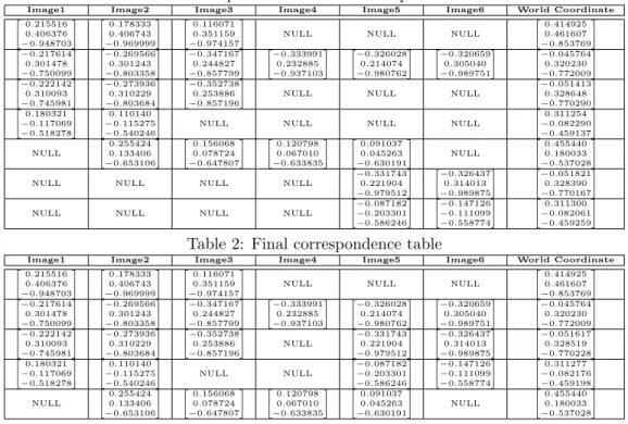
Table 2: Final correspondence table
Image1 Image2 Image3 Image4 Image5 Image6 World Coordinate 0.215516 0.406376 −0.948703 0.178333 0.406743 −0.969999 0.116071 0.351159 −0.974157
NULL NULL NULL
0.414925 0.461607 −0.853769 −0.217614 0.301478 −0.750099 −0.269566 0.301243 −0.803358 −0.347167 0.244827 −0.857799 −0.333991 0.232885 −0.937103 −0.326028 0.214074 −0.980762 −0.320659 0.305040 −0.989751 −0.045764 0.320230 −0.772009 −0.222142 0.310093 −0.745981 −0.273936 0.310229 −0.803684 −0.352738 0.253886 −0.857196 NULL −0.331743 0.221904 −0.979512 −0.326437 0.314013 −0.989875 −0.051617 0.328519 −0.770228 0.180321 −0.117069 −0.518278 0.110140 −0.115275 −0.540246 NULL NULL −0.087182 −0.203301 −0.586246 −0.147126 −0.111099 −0.558774 0.311277 −0.082176 −0.459198 NULL 0.255424 0.133406 −0.653106 0.156068 0.078724 −0.647807 0.120798 0.067010 −0.633835 0.091037 0.045263 −0.630191 NULL 0.455440 0.180033 −0.537028
initial estimate of the 3D world coordinate points. Table 1 shows a few rows of a correspondence table. This search across image pairs can be done efficiently recognizing that the number of correspondences is relatively small, and once correspondences are entered into the table, they can be removed from further consideration.
Once the initial correspondence table is created, each row of the table is compared with all other rows to check if any of those rows belong to the same point in the world coordinate system. To meet this condition, each column should not have entries in both rows and the Euclidean distance between two points in the world coordinate system has to be less than a threshold. If these conditions are met, two rows are merged together and the 3D point in world coordinates is recomputed. At the end of this pass, the table contains the initial estimate of the 3D points in the world coordinate system and the corresponding points in each image space if it is visible. The final 3D points will be the initial estimates used in the bundle adjustment process. Table 2 shows the rows of the final correspondence table after merging the third row with the sixth row and the fourth row with the seventh row of the initial correspondence table. The distance between the 3D points in a row when mapped into world coordinates is less than the threshold and hence they are the same points in the world coordinate system.
4. BUNDLE ADJUSTMENT
After the formation of the correspondence table, the 3D points and the individual SOPs are optimized so that
the error is minimized. Each 3D pointi in the world coordinate system can be transformed into each image
spacej using the inverse SOP transformation given by
ˆ Xji= ˆ xji ˆ yji ˆ zji = 1− 2(q2j2+qj32) q2 j0+q2j1+qj22+q2j3 2(qj1qj2−qj0qj3) q2 j0+qj12+q2j2+q2j3 2(qj1qj3+qj0qj2) q2 j0+q2j1+qj22+qj32 2(qj1qj2+qj0qj3) q2 j0+q2j1+qj22+q2j3 1− 2(qj12+q2j3) q2 j0+qj12+q2j2+q2j3 2(qj2qj3−qj0qj1) q2 j0+q2j1+qj22+qj32 2(qj1qj3−qj0qj2) q2 j0+q2j1+qj22+q2j3 2(qj2qj3+qj0qj1) q2 j0+qj12+q2j2+q2j3 1− 2(q2j2+q2j1) q2 j0+q2j1+q2j2+qj32 T bix−tjx biy−tjy biz−tjz , (5) where bi = [bix, biy, biz] T
are the 3D points in the world coordinate system, qj0, qj1, qj2, qj3 are the
quater-nions derived from the rotation matrix, and tj = [tjx, tjy, tjz]
T
are the 3D translation vectors.12 Normalized
aj = [qj0, qj1, qj2, qj3, tjx, tjy, tjz]
T
define the SOPs from the jth image to the world coordinate system. If
X = [xji, yji, zji]T are the actual 3D correspondences in the image space, then the total squared error of the system is given by E2= n−1 X j=0 m−1 X i=0 h (xji−xˆji) 2 + (yji−yˆji) 2 + (zji−zˆji) 2i (6)
forn images andm 3D world points. If ith 3D point is not visible injth image, then those terms are simply
omitted from the sum.
The goal of the optimization is to reduce this error. Since the function that takes the 3D point in world space to image space is highly nonlinear, a nonlinear optimization technique must be used. Bundle adjustment is a technique to jointly estimate the SOP parameters and the 3D points so as to minimize the error of the system. One popular method to do bundle adjustment is Levenberg-Marquardt algorithm (LMA).
The sparse LMA described by Hartley and Zisserman1 is used to adjust both the SOP parameters and 3D
points to fit one another. This is because the correspondences might also contains some measurement error.
This method jointly optimize minimizing the error and fitting the data to the model. IfP = (aT,bT) is the
parameter vector andX is the measurement vector, the general function which takes the parameter vector to
the measurement vector isXˆ =f(P). If we denoteE =X−Xˆ error between the measured and estimate, we
seek to minimized the square distancekEk2=ETE given in (6).
In a multiple SOP system, the parametera can be partitioned asa = [aT1,aT2, . . . ,aTm]. There is a lack of
interaction between parameters of different SOPs, so the normal equation which is the main computation in bundle adjustment will have a sparse “skyline” structure.
5. REGISTRATION RESULTS
The algorithm described above was tested with two kinds of texel images, synthetic and real images captured from a texel camera. Six synthetic texel images were created of a scene of about a square meter in size, and
Gaussian noise withσ = 0.5 cm was added to the lidar range values of the image. The images are created in
such a way that they contain many features. This is to validate the algorithm, which can be ineffective if there are very few features. The pairwise registration was done first, and individual SOPs were calculated. After the pairwise registration, the correspondence table was created, and the LM algorithm was performed to reduce the error given by (6). The initial estimates for the points in world coordinates were taken from the correspondence table, and the initial estimates for the SOPs were taken from the pairwise registration.
The results of the registration are shown in Figure 1. The images are rendered in a 3D viewer designed to
display the best textures from the set of images depending on the viewpoint,13and the black areas correspond to
missing data in the texel images or textures with large range error. Two different views are shown to indicate the 3D nature of the texel images. It is interesting to note that even with 0.5 cm error in the 3D measurements, the pairwise registration is visually good, and the effects of bundle adjustment don’t show much visual improvement. The error was reduced only by half due to bundle adjustment.
A texel camera was used to capture six images of a scene from different viewpoints. The texel camera can produce significant range error on sharp edges, so this test is a challenge to the algorithm. The pairwise registration was performed on the images and the correspondence table formed. The correspondences found by the algorithm are illustrated in Figure 2. Only about half of the correspondence points found are shown for clarity purposes. The bundle adjustment was then performed. The convergence plot of the bundle adjustment is given in Figure 3. Note that the error was reduced by about 75% using bundle adjustment.
The visual results of the registration are given in Figure 4. Careful evaluation of the images indicates that both the pairwise regestered and the bundle adjusted registration gave good results. The bundle adjusted images are visually better registered, as indicated by the checkerboard surface of the cube and the writing on the objects. A final test was run on the captured texel images. The first image in the set was added at the end of the sequence, and the algorithm run on the seven images. Since the starting and ending images were identical (and
(a) (b)
(c) (d)
Figure 1: Registration results for the synthetic texel images. (a) Pairwise registered. (b) LM bundle adjusted. (c) Pairwise registered from a second view. (d) LM bundle adjusted from a second view.
Figure 2: Corresponding points in each of the captured texel images, joined by a line. Different colors indicate common correspondences.
0 50 100 150 200 250 300 350 400 450 500 1 2 3 4 5 6 7 8x 10 −6 Iteration Mean−squared Error
Figure 3: Error at each LM iteration for the captured texel images.
(a) (b)
(c) (d)
Figure 4: Registration results for the captured texel images. (a) Pairwise registered. (b) LM bundle adjusted. (c) Pairwise registered from a second view. (d) LM bundle adjusted from a second view.
from identical perspectives), the computed SOPs should be identical. To measure the accuracy of the registration, the Frobenious norm of the difference between the starting and ending SOPs was computed, and found to be 0.0372 for pairwise registration, and 0.0286 after bundle adjustment, a reduction of about 23%.
6. CONCLUSION
The methods described in this paper have shown that registration of several texel images consisting of fused image and lidar data is successful by exploiting the properties of both datasets simultaneously. The registra-tion was performed without any prior knowledge of the perspectives of the images, and produces a very good registration using both pairwise and bundle adjustment methods. Key to the success of the algorithm is the automatic selection of correspondences using both 2D and 3D criteria within the RANSAC outlier removal. Photogrammetric methods alone have no measured 3D information, and 3D registration methods (such as ICP) are susceptible to convergence issues. The method presented here overcomes both deficiencies.
One surprising outcome of these experiments is the quality of the pairwise registration. Bundle adjustment is often applied to reduce cumulative error when registering a set of images, but showed measurable but small improvement in these experiments. Further experimentation is needed with a larger set of images to quantify the benefit.
REFERENCES
[1] Hartley, R. and Zisserman, A., [Multiple view geometry in computer vision], Cambridge University Press
(2003).
[2] Hahne, U. and Alexa, M., “Combining time-of-flight depth and stereo images without accurate extrinsic
calibration,” Int. J. Intell. Syst. Technol. Appl.5, 325–333 (Nov. 2008).
[3] Stamos, I. and Allen, P. K., “Integration of range and image sensing for photorealistic 3d modeling,” in
[Proc. IEEE Int. Conf. Robotics and Automation], 1435–1440 (2000).
[4] Ko, R. K., Nishino, K., Zhang, Z., and Ikeuchi, K., “Simultaneous 2d images and 3d geometric model
registration for texture mapping utilizing reflectance attribute,” in [Proc. Fifth Asian Conf. on Computer
Vision], 99–106 (2002).
[5] Umeda, K., Godin, G., and Rioux, M., “Registration of range and color images using gradient constraints
and range intensity images,” in [Proc. Int. Conf. Pattern Recogition], 3, 12–15 Vol.3 (Aug 2004).
[6] Budge, S. E. and Badamikar, N. S., “Calibration method for texel images created from fused lidar and
digital camera images,”Opt. Eng.52, 103101–103101 (Oct. 2013).
[7] Budge, S. E., Badamikar, N. S., and Xie, X., “Automatic registration of fused lidar/digital imagery (texel
images) for three-dimensional image creation,” Opt. Eng.54, 031105 (Mar. 2015).
[8] Bybee, T. C. and Budge, S. E., “Textured digital elevation model formation from low-cost UAV ladar/digital
image data,” in [Laser Radar Technology and Applications XX], Turner, M. D. and Kamerman, G. W., eds.,
9465, 94650H–94650H–12, SPIE, Baltimore, Maryland, USA (May 2015).
[9] Harris, C. and Stephens, M., “A combined corner and edge detector.,” in [Proc. of Fourth Alvey Vision
Conference], 147–151 (1988).
[10] Noble, J. A.,Descriptions of image surfaces, PhD thesis, University of Oxford (1989).
[11] Fischler, M. A. and Bolles, R. C., “Random sample consensus: a paradigm for model fitting with applications
to image analysis and automated cartography,”Communications of the ACM24(6), 381–395 (1981).
[12] Horn, B. K., “Closed-form solution of absolute orientation using unit quaternions,”JOSA A4(4), 629–642
(1987).
[13] Killpack, C. and Budge, S. E., “Visualization of 3D images from multiple texel images created from fused
lidar/digital imagery,” in [Laser Radar Technology and Applications XX], Turner, M. D. and Kamerman,