Learning a multi-branch neural network from multiple sources for knowledge adaptation in remote sensing imagery

(1)

remote sensing

Article

Learning a Multi-Branch Neural Network from

Multiple Sources for Knowledge Adaptation in

Remote Sensing Imagery

Mohamad M. Al Rahhal1 , Yakoub Bazi2,* , Taghreed Abdullah3, Mohamed L. Mekhalfi4, Haikel AlHichri2 _{and Mansour Zuair}2

1 _{Information Science Department, College of Applied Computer Science, King Saud University,} Riyadh 11543, Saudi Arabia; [email protected]

2 _{Computer Engineering Department, College of Computer and Information Sciences, King Saud University,} Riyadh 11543, Saudi Arabia; [email protected] (H.A.); [email protected] (M.Z.)

3 _{Department of Studies in Computer Science, University of Mysore, Mysore 570006, India;} [email protected]

4 _{Department of Electronics, Faculty of Technology, University of Batna, Batna 05000, Algeria;} [email protected]

* Correspondence: [email protected]; Tel.: +966-1014696297

Received: 3 October 2018; Accepted: 23 November 2018; Published: 27 November 2018 Abstract: In this paper we propose a multi-branch neural network, called MB-Net, for solving the problem of knowledge adaptation from multiple remote sensing scene datasets acquired with different sensors over diverse locations and manually labeled with different experts. Our aim is to learn invariant feature representations from multiple source domains with labeled images and one target domain with unlabeled images. To this end, we define for MB-Net an objective function that mitigates the multiple domain shifts at both feature representation and decision levels, while retaining the ability to discriminate between different land-cover classes. The complete architecture is trainable end-to-end via the backpropagation algorithm. In the experiments, we demonstrate the effectiveness of the proposed method on a new multiple domain dataset created from four heterogonous scene datasets well known to the remote sensing community, namely, the University of California (UC-Merced) dataset, the Aerial Image dataset (AID), the PatternNet dataset, and the Northwestern Polytechnical University (NWPU) dataset. In particular, this method boosts the average accuracy over all transfer scenarios up to 89.05% compared to standard architecture based only on cross-entropy loss, which yields an average accuracy of 78.53%.

Keywords:scene classification; multiple sources; multiple domain shifts; multi-branch neural network

1. Introduction

Over the last two decades remote sensing has become a staple technology for monitoring urban, atmospheric, and ecological changes [1,2]. One of the prominent and arguably most active areas in this context refers to scene classification, which enables pinpointing of the semantic tenor of a geographical area of interest. This may come with the cost of processing large masses of data (e.g., multispectral and hyperspectral images) that are often manifested in voluminous spectral layers, alongside a wide spatial context. On the other hand, the mainstream literature so far suggests that scene classification can be tackled from two perspectives. First, the earliest works in this regard tend to classify image pixels [3–5], typically by handling raw spectral values along with neighbouring attributes. The second approach is based on scene-level recognition [6–8], which has received interest recently, thanks to its property of offering broader semantic information.

(2)

Remote Sens.2018,10, 1890 2 of 18

In view of the two trends mentioned above, an efficient classification system lies in determining how to mitigate the semantic gap between low level image features on the one hand, and their respective semantic attributes, on the other. Thus, a typical classification pipeline would extract handcrafted features and feed them into a classifier, which has been shown to address the problem to some extent [9,10]. For instance, a multiresolution representation bag of visual words (BOVW) model was presented [11]. For an improved classification, a feature fusion by means of compressive sensing was introduced [12]. Additionally, a correlation model was developed [13], which takes into consideration pixel homogeneity. A feature extraction method has been proposed, which relies on multi-scale completed local binary patterns [14]. Additionally, a pyramid-of-spatial-relations model was introduced to combine both relative and absolute spatial information into the BOVW model for the scene classification problem [15]. In another work, the authors introduced a method based on Gabor filters and the completed local binary patterns operator [16].

The amount of remote sensing images has been steadily increasing due to the technological improvement of satellite sensors [17]. Thus, massive volumes of images with different spectral channels and spatial resolutions can be obtained [18]. How to recognize and analyze such images has become a big challenge [19]. Nowadays, plenty of work concentrates on deep learning strategies based on convolutional neural networks (CNNs), which aim to learn, in an end-to-end manner, representative as well as discriminative features automatically. Thanks to their sophisticated structure, these models have the ability to learn powerful generic image representations in a hierarchical fashion. The impressive results obtained on several remote sensing scene datasets confirm clearly their superiority compared to shallow methods based on handcrafted features [20–29].

In some domains there are sufficient labeled samples to train a classification model, whereas many new domains lack labeled samples [30]. Moreover, generating and collecting labeled data is often expensive and time consuming [31]. As a result, the idea of exploiting the availability of labeled data in one or more domain to predict unlabeled data in another domain has emerged, and is known as “domain adaptation”. Unlike several machine learning algorithms, which assume that the training and testing samples are drawn from the same distribution [32], training and testing data in domain adaptation have different distributions, that is, the training images are always with labels and are extracted from what is called the source domain, while the test images are without (or with few) labels and are called the target domain [1]. The main goal of domain adaptation is to mitigate the distribution discrepancy between the source and target domains [33]. It is worth recognizing that domain adaptation has been applied in various applications such as computer vision [34], sentimental analysis [35], natural language processing [36,37], video concept detection [38], and Wi-Fi localization and detection [39].

In the literature of computer vision, many works have shown that deep networks can learn more transferable features for domain adaptation. As a result, domain adaptation methods learn deep neural transformations that map both domains into a common feature space. In [40], a unified deep adaptation framework is proposed for jointly learning transferable representation and classifier to enable scalable domain adaptation, by leveraging both deep learning and optimal two-sample matching. In [41], to reduce domain discrepancy an adaptation layer is added to the deep convolutional neural network (CNN) to achieve lower transfer errors. In another work [42], deep adaptation network (DAN) model is proposed, which gave state of the art results. In [43], to produce the commonality between the source and target distributions and accommodate the domain-specific parts that should not be aligned, local patches of varying sizes are extracted and processed via CNNs. In [44], transformation between the source and target is proposed to be learnt by the deep model regression network. Based on the nature of CNNs, this approach presumes that the source representation can be interpolated or regressed into the target, as it can approximate highly non-linear functions. In another work [45], a deep domain adaptation network is presented for the problem of describing people based on fine-grained clothing attributes. Specifically, an improved version of the Region CNN body detector is introduced, which effectively localizes the clothing area. In fact, it consists of three sub-modules. First, a selective search is

(3)

Remote Sens.2018,10, 1890 3 of 18

utilized to generate candidate region proposals. Then, a Network in Network model is used to extract features for each candidate region. Finally, linear support vector regression is exploited to predict the Intersection over Union overlap of candidate patches with ground-truth bounding boxes. In [46], the authors trained a network to do both feature and classifier adaptation. Analogous to previous domain adaptation methods, feature adaptation is accomplished by matching the distributions of features across domains. Nevertheless, unlike prior works, the presented method allows classifier adaptation by adding a residual transfer module that bridges the source and target classifiers. The adaptation can be used in most feed-forward models by extending them with new residual layers and loss functions, which can be trained efficiently via back-propagation. In another work, a deep coral technique was proposed to mitigate the domain discrepancy for enhancing the classification procedure of CNN by reducing the Euclidean distance between covariance matrices in the source and target domains [47]. Yet it is not certain if the Euclidean distance is a typical choice for minimizing the distance between both domains. Therefore, to deal with this issue, the work in [48] presented a new deep Log-coral method, which used geodesic distance rather than Euclidean distance. The obtained accuracies have demonstrated the effectiveness of minimizing geodesic distance instead of using simple Euclidean distance on covariance matrices. Lately, adversarial approaches to unsupervised domain adaptation have been introduced to improve generalization performance by reducing the discrepancy between the training and test domain distributions. The authors in [49] adopted an inverted label adversarial network loss to divide the optimization into two independent objectives, one for the generator and one for the discriminator, by comparing them relying on the loss type, and the weight sharing strategy between the two streams.

With respect to domain adaptation with multiple sources, some contributions based on handcrafted features have been published. The work in [50] aims to maximize unanimity of predictions from multiple sources, although not all source domains may be useful for knowledge adaptation. In [51], a kernel mean matching technique was adopted to match the means of different domains. The work in [52] proposed to combine multiple auxiliary classifiers trained on source data to classify target data. In [53], a smoothness regularizer is used to weight different source domains. In [54], it was assumed that the distributions of multiple sources are similar, but the labelled samples from different sources may be different from each other. In [55], a clustering based scheme was proposed to divide a dataset into latent domain, which is further extended in [56] for multi-domain adaptation. The work in [57] presented an event recognition method for consumer videos by leveraging web videos from YouTube, in order to handle the mismatch between data distributions of two domains (i.e., web video domain and consumer video domain).

In the context of remote sensing, in the literature there are few works related to single source domain adaptation approaches based on deep learning techniques and mainly related to cross-scene classification. By cross-scene classification, we mean datasets acquired with different sensors and over different locations (i.e., training and testing images are taken from two different scene datasets). Under this assumption, the data-shift problem should be considered alongside the representation aspect to obtain satisfactory results. For example, Othman et al. [58] added additional regularization terms to the objective function of the neural network besides the standard cross-entropy loss, in order to compensate for the distribution mismatch to alleviate the low accuracies resulting from the approaches relying on pre-trained CNNs. In [59], the authors developed an approach based on adversarial networks for cross-domain classification in aerial vehicle images to overcome the data shift problem. Finally, the authors in [60] addressed this issue by projecting the source domain samples to the target domain via a regression network, while keeping the discrimination ability of the source samples.

Although multisource domain adaptation has been shown to be very useful in general computer vision literature, it is yet to find its way into remote sensing applications. To the best of our knowledge, there is still no contribution on multisource domain adaptation for the specific task of scene classification. This could be traced back to the fact that, years ago, remote sensing did not benefit from multiple scene classification datasets that shared an adequate number of object classes.

(4)

Remote Sens.2018,10, 1890 4 of 18

However, thanks to recent efforts made by researchers, several benchmark scene datasets are now available to the community of remote sensing, which opens the door to development of advanced methodologies such as those related to multisource domain adaptation.

In this work, we propose a multi-branch neural network called MB-Net for solving the problem of knowledge adaptation from multiple scene datasets sharing the same number of object classes. Specifically, our aim is to learn invariant feature representations from multiple source scene datasets with labeled images and one target scene dataset with unlabeled images. For this purpose, we define for the network an objective function that allows to mitigate the multiple domains shifts at both feature representation and decision levels, while keeping the discrimination ability between different object classes. The complete architecture is trainable end-to-end via the backpropagation algorithm. In the experiments, we demonstrate the effectiveness of the proposed method on a new multiple domain scene dataset created from four heterogonous scene datasets: the University of California (UC-Merced) dataset [61], Aerial Image Dataset (AID) [62], PatternNet dataset [63], and finally, the Northwestern Polytechnical University (NWPU) dataset [64].

The paper is organized as follows: Section2describes the proposed method. Section3shows the results obtained on the multiple source scene dataset. Section4analyzes the sensitivity of the method and presents some comparisons with some recent state-of-the-art methods based on deep neural networks. Finally, Section5draws conclusions and future developments.

2. Description of the Proposed Method 2.1. Preliminaries Let us considerSk= n X(sk) i ,y (s_k) i on_sk

i=1,k=1, 2, . . . ,Mas the dataset from thek-th source domain

withnsklabeled images, whereMrepresents the number of source domains. Here,X

(s_k) i andy

(s_k) i are the images in thek-th source domain and their corresponding class labelsy(sk)

i ∈ {1, 2, . . . ,J}, whereJ is the number of classes. Also, let us consider a single target datasetT=nX(t)_j ont

j=1composed ofnt

unlabeled images. As mentioned in the introduction section, the main contribution of this work is to develop an MB-Net architecture (Figure1) that captures the shared knowledge across different labeled source datasetsSkand generalizes well on the new unlabeled target datasetT.

Remote Sens. 2018, 10, x FOR PEER REVIEW 4 of 19

However, thanks to recent efforts made by researchers, several benchmark scene datasets are now available to the community of remote sensing, which opens the door to development of advanced methodologies such as those related to multisource domain adaptation.

In this work, we propose a multi-branch neural network called MB-Net for solving the problem of knowledge adaptation from multiple scene datasets sharing the same number of object classes. Specifically, our aim is to learn invariant feature representations from multiple source scene datasets with labeled images and one target scene dataset with unlabeled images. For this purpose, we define for the network an objective function that allows to mitigate the multiple domains shifts at both feature representation and decision levels, while keeping the discrimination ability between different object classes. The complete architecture is trainable end-to-end via the backpropagation algorithm. In the experiments, we demonstrate the effectiveness of the proposed method on a new multiple domain scene dataset created from four heterogonous scene datasets: the University of California (UC-Merced) dataset [61], Aerial Image Dataset (AID) [62], PatternNet dataset[63], and finally, the Northwestern Polytechnical University (NWPU) dataset [64].

The paper is organized as follows: Section 2 describes the proposed method. Section 3 shows the results obtained on the multiple source scene dataset. Section 4 analyzes the sensitivity of the method and presents some comparisons with some recent state-of-the-art methods based on deep neural networks. Finally, Section 5 draws conclusions and future developments.

2. Description of the Proposed Method

2.1. Preliminaries

Let us consider 𝑆 = 𝑋( ), 𝑦( ) , 𝑘 = 1, 2, … , 𝑀 as the dataset from the 𝑘-th source domain with 𝑛 labeled images, where 𝑀 represents the number of source domains. Here, 𝑋( ) and 𝑦( ) are the images in the 𝑘-th source domain and their corresponding class labels 𝑦( )∈ 1,2, … , 𝐽 , where

𝐽 is the number of classes. Also, let us consider a single target dataset 𝑇 = 𝑋( ) composed of 𝑛 unlabeled images. As mentioned in the introduction section, the main contribution of this work is to develop an MB-Net architecture (Figure 1) that captures the shared knowledge across different labeled source datasets 𝑆 and generalizes well on the new unlabeled target dataset 𝑇.

Figure 1. Proposed MB-Net architecture: Pre-trained convolutional neural networks (CNN) coupled with additional branches, where each branch is related to a specific source dataset 𝑆 .

Figure 1.Proposed MB-Net architecture: Pre-trained convolutional neural networks (CNN) coupled with additional branches, where each branch is related to a specific source datasetSk.

(5)

Remote Sens.2018,10, 1890 5 of 18

2.2. Model Architecture

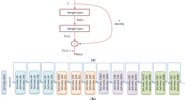
MB-Net is based on a pre-trained CNN coupled with additional branches. As a pre-trained CNN, we use the residual network (ResNet) [65], which is based on the idea of identity shortcut connection. In particular, we use ResNet50, which is a 50-layer network with a 3-layer bottleneck block (Figure2). ResNet has been introduced to solve the vanishing gradients problems in deeper networks. It introduces the idea of learning residual functions with reference to the layer inputs rather than learning unreferenced functions (see Figure2). ResNet won first place in the ImageNet Large Scale Visual Recognition Competition (ILSVRC) 2015 classification completion. It has been used to replace the VGG-16 layers in the faster Region CNN (RCNN) learning for better improvements in terms detection results. In this work, we use this ResNet50 pre-trained on the well-known ImageNet dataset as the first module in our network.

2.2. Model Architecture

MB-Net is based on a pre-trained CNN coupled with additional branches. As a pre-trained CNN, we use the residual network (ResNet) [65], which is based on the idea of identity shortcut connection. In particular, we use ResNet50, which is a 50-layer network with a 3-layer bottleneck block (Figure 2). ResNet has been introduced to solve the vanishing gradients problems in deeper networks. It introduces the idea of learning residual functions with reference to the layer inputs rather than learning unreferenced functions (see Figure 2). ResNet won first place in the ImageNet Large Scale Visual Recognition Competition (ILSVRC) 2015 classification completion. It has been used to replace the VGG-16 layers in the faster Region CNN (RCNN) learning for better improvements in terms detection results. In this work, we use this ResNet50 pre-trained on the well-known ImageNet dataset as the first module in our network.

We remove the softmax layer and take the output of the average pooling layer (feature vector of dimension 2048) as input to different branches. Each branch related to a specific source dataset is composed of two dense layers of size 128. Each dense layer is followed by batch normalization (BN), linear rectified unit (ReLU) activation function, and dropout regularization. On top of these dense layers, we place a softmax classification layer (Figure 3). Additionally, to reduce the discrepancy between the source and target distributions, our network has average pooling layers 𝐴 and 𝐴 placed after the first dense layer and the softmax layer, respectively.

(a)

(b)

Figure 2. (a) Residual block; and (b) architecture of ResNet50.

Figure 3. One branch of MB-Net related to the k-th source domain.

Figure 2.(a) Residual block; and (b) architecture of ResNet50.

We remove the softmax layer and take the output of the average pooling layer (feature vector of dimension 2048) as input to different branches. Each branch related to a specific source dataset is composed of two dense layers of size 128. Each dense layer is followed by batch normalization (BN), linear rectified unit (ReLU) activation function, and dropout regularization. On top of these dense layers, we place a softmax classification layer (Figure3). Additionally, to reduce the discrepancy between the source and target distributions, our network has average pooling layersAv1andAv2

placed after the first dense layer and the softmax layer, respectively.

2.2. Model Architecture

MB-Net is based on a pre-trained CNN coupled with additional branches. As a pre-trained CNN, we use the residual network (ResNet) [65], which is based on the idea of identity shortcut connection. In particular, we use ResNet50, which is a 50-layer network with a 3-layer bottleneck block (Figure 2). ResNet has been introduced to solve the vanishing gradients problems in deeper networks. It introduces the idea of learning residual functions with reference to the layer inputs rather than learning unreferenced functions (see Figure 2). ResNet won first place in the ImageNet Large Scale Visual Recognition Competition (ILSVRC) 2015 classification completion. It has been used to replace the VGG-16 layers in the faster Region CNN (RCNN) learning for better improvements in terms detection results. In this work, we use this ResNet50 pre-trained on the well-known ImageNet dataset as the first module in our network.

We remove the softmax layer and take the output of the average pooling layer (feature vector of dimension 2048) as input to different branches. Each branch related to a specific source dataset is composed of two dense layers of size 128. Each dense layer is followed by batch normalization (BN), linear rectified unit (ReLU) activation function, and dropout regularization. On top of these dense layers, we place a softmax classification layer (Figure 3). Additionally, to reduce the discrepancy between the source and target distributions, our network has average pooling layers 𝐴 and 𝐴 placed after the first dense layer and the softmax layer, respectively.

(a)

(b)

Figure 2. (a) Residual block; and (b) architecture of ResNet50.

Figure 3. One branch of MB-Net related to the k-th source domain.

(6)

Remote Sens.2018,10, 1890 6 of 18

2.3. Objective Function and Model Optimization

Let us defineΘsk_{as the weights and biases associated with the different branches of the network.}

To learn these parameters, we propose to minimize an objective function composed of three terms:

LX(sk)_,_X(t)_,Θsk₌_L_ce₊_λ 1Lh+λ2Lo (1) Lce=

∑

_k=M₁ − 1 nsk

∑

n_sk i=1

∑

J j=11(yi =j)logP yi =j X (s_k)_,_Θs_k , (2) Lh=k 1 ns

∑

ns i=1h (s)₋ 1 nt

∑

nt j=1h (t)_k2 2, (3) Lo =k 1 ns

∑

ns i=1O (s)₋ 1 nt

∑

nt j=1O (t)_k2 2. (4)

whereλ1andλ2are two regularization parameters (set to 1 in the experiments). The termLcerepresents the total cross-entropy loss computed for theM-labeled source datasets; 1(·)is an indicator function that takes 1 if the statement is true, otherwise it takes 0; andPyi= j

X (s_k)_,_Θsk is the probability output vector provided by the softmax regression layer of thek-th source domain. The termLhis the distance between the source and target domains computed at the hidden representation layer of the network, as shown in Figure1. The termsh(s)andh(t)refer to the feature representations of the source and target domains generated by the average layerAv1. Similarly, the termLois the distance between the source and target domains computed at the output of the network. Here,O(s)_and_O(t) _{refer to} the outputs of the source and target domains generated by the average layerAv2placed on top of the

softmax regression layers.

To optimize the above loss functions, one can use the backpropagation algorithm and the mini-batch classical stochastic gradient descent (SGD) method. The learning process starts by pre-training the network on the labeled source domains by optimizing the cross-entropy lossLce. This is done by dividing the source domains into several mini-batches of the same size, afterwhich learning is performed by updating the weights for every mini-batch as follows:

Θsk ₌Θsk₋ η bsk rnsk_b

∑

i=1+(r−1)nsk_b dLce X(sk) r dΘsk (5)

whereηrefers to the learning rate,bsk _and_nsk

b refer to the size and number of mini-batches in thek-th source, respectively. Then, in the second phase we fine tune the network weights by minimizing the complete lossLusing both the source and target domains. Mathematically, the weights of the network are then updated as follows:

Θsk ₌Θsk₋ η b rn_b

∑

i=1+(r−1)nb   dLce X(sk) rand dΘsk +λ1 dLh X(sk) rand,X (t) i dΘsk +λ1 dLo X(sk) rand,X (t) i dΘsk   (6)

where b and nb refer to the size and the number of mini-batches in the target domain. During the learning process, random samplesX(sk)

randare extracted from the different sources to reduce the discrepancy between the domains while keeping the discrimination ability of the network.

It is worth recalling that for better performances, we use in the experiments more advanced gradient-based update rules based on the mini-batch adaptive moment estimation (Adam) method for updating the parameters The Adam method is an extension of the SGD method. While SGD maintains a single learning rate for all weights during the training process, the Adam method computes individual adaptive learning rates for different parameters from estimates of first- and second-order moments of the gradients, which makes it very efficient.

(7)

Remote Sens.2018,10, 1890 7 of 18

The following algorithm provides the main steps for training MB-Net with its nominal parameters:

MB-Net method.

Input: Source domainsSk= n X(sk) i ,y (sk) i on_sk

i=1, k=1, . . . ,Mand one target domainT= n

X_i(t)ont i=1

Output: Target class labels 1: Set MB-Net parameters:

• Regularization parametersλ1=λ2=1 • Mini-batch size:b=100

• Adam parameters: learning rateη= 0.001, exponential decay rate for the first and second moments β1=0.9,β2=0.999 and epsilon = 1 ×10−8

2: Pre-train the network on theM-labeled source domains using the Adam method (i.e., estimate the parametersΘsk_{by optimizing only the cross-entropy loss}_Lce_{in Equation (2))}

3: Set the number of mini-batches:n_b=nt/b 4: Forepoch=1 : num_epoch

4.1 Shuffle randomly the unlabeled target images and organize them intonbgroups each of sizeb 4.2 Forr=1 : nb

• Pick a mini-batchrfrom the target domain:Tr(t)= n

X(_it)ornb

i=1+(r−1)nb

• Feed this mini-batch to the different branches of the network and take the outputh(rt)andOr(t)of the average pooling layerAv1andAv2, respectively

• Pick randomlyMmini-batch from the source domainsX(sk)

rand,k=1, . . . ,M

• Feed each source mini-batch to its corresponding branch and take the outputh(_rands) andOrand(s)of the average layersAv1andAv2, respectively

• Update the parametersΘsk _{of the network by minimizing the total loss}_L₌_L

ce+λ1Lh+λ2Lo (Equation (1)) on the current mini-batch

5: Classify the target domainT.

3. Experimental Results

3.1. Description of the Multisource Dataset

To assess the performance of the proposed approach we use four heterogonous scene remote sensing datasets, collected and labeled by different experts to build the multisource dataset. These are the Merced, AID, PaternNet and NWPU datasets. This setting corresponds to three labeled source domains and one unlabeled target domain.

The Merced dataset is widely used for the task of aerial image classification. It is composed of 21 classes with 100 RGB images of size 256×256 pixels each, with 30 cm pixel resolution. This dataset was extracted from the United States Geological Survey (USGS) National Map Urban Area Imagery collection, from various urban areas pertaining to the following US regions: Birmingham, Boston, Buffalo, Columbus, Dallas, Harrisburg, Houston, Jacksonville, Las Vegas, Los Angeles, Miami, Napa, New York, Reno, San Diego, Santa Barbara, Seattle, Tampa, Tucson, and Ventura. The dataset amounts to 2100 images manually selected and labelled into 21 classes: agricultural, airplane, baseball diamond, beach, buildings, chaparral, dense residential, forest, freeway, golf course, harbor, intersection, medium density residential, mobile home park, overpass, parking lot, river, runway, sparse residential, storage tanks, and tennis courts.

The AID dataset is made up of 10,000 large-scale aerial images of size 600×600 pixels with multi-resolution (8 m to 0.5 m) within the following 30 aerial scene kinds: airport, bare land, baseball field, beach, bridge, center, church, commercial, dense residential, desert, farmland, forest, industrial, meadow, medium residential, mountain, park, parking, playground, pond, port, railway station,

(8)

Remote Sens.2018,10, 1890 8 of 18

resort, river, school, sparse residential, square, stadium, storage tanks and viaduct. Specialists in the field of remote sensing image interpretation annotated all the images, which are multi-source (from different remote sensing imaging sensors). Furthermore, the images of each class are carefully collected from various countries and areas around the world, including England, the United States, Germany, Italy, China, Japan, etc., and they are obtained at different times and seasons under different imaging circumstances.

The PatternNet dataset is collected from Google Earth imagery for remote sensing image retrieval, and consists of 38 classes: airplane, baseball field, basketball court, beach, bridge, cemetery, chaparral, Christmas tree farm, closed road, coastal mansion, crosswalk, dense residential, ferry terminal, football field, forest, freeway, golf course, harbor, intersection, mobile home park, nursing home, oil gas field, oil well, overpass, parking lot, parking space, railway, river, runway, runway marking, shipping yard, solar panel, sparse residential, storage tank, swimming pool, tennis court, transformer station and wastewater treatment plant. Each class comprises 800 images of size 256×256 pixels.

The NWPU dataset is collected by Northwestern Polytechnical University (NWPU). It accommodates 31,500 images corresponding to 45 scene classes with 700 images in each class of size 256×256 pixels. The spatial resolution of the images in each class varies from about 0.2 to 30 m. These 45 scene classes include airplane, airport, baseball diamond, basketball court, beach, bridge, chaparral, church, circular farmland, cloud, commercial area, dense residential, desert, forest, freeway, golf course, ground track field, harbor, industrial area, intersection, island, lake, meadow, medium residential, mobile home park, mountain, overpass, palace, parking lot, railway, railway station, rectangular farmland, river, roundabout, runway, sea ice, ship, snow berg, sparse residential, stadium, storage tank, tennis court, terrace, thermal power station, and wetland.

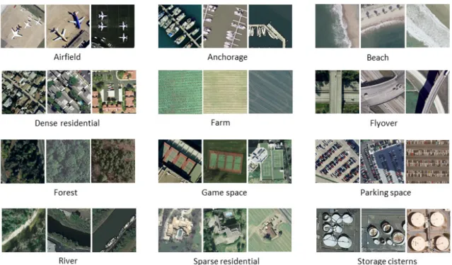
To make these datasets suitable for multisource domain adaptation, we consider in this work only the shared classes across them and discard the remainders. After this pre-processing step, we obtained twelve shared classes as shown in Table 1, which are airfield, anchorage, beach, dense residential, farm, flyover, forest, game space, parking space, river, sparse residential, and storage tanks. Figures 4–7 show sample images related to these shared classes for the four datasets, respectively. In the experiments, we refer to the four possible transfer scenarios as follows:(SMerced,SNWPU,SPatNet)→TAID, (SAID,SNWPU,SPatNet)→TMerced,

(SAID,SMerced,SPatNet)→TNWPU, and(SAID,SMerced,SNWPU)→TPatNet.

Table 1.Shared classes extracted from Merced, AID, PatternNet, and NWPU datasets.

Class Merced AID PatternNet NWPU

Airfield 100 360 800 1400 Anchorage 100 380 800 700 Beach 100 400 800 700 Dense Residential 100 410 800 700 Farm 100 370 800 1400 Flyover 100 420 800 700 Forest 100 250 800 700 Game Space 100 660 1600 1400 Parking Space 100 390 800 700 River 100 410 800 700 Sparse Residential 100 300 800 700 Storage Cisterns 100 360 800 700 Total 1200 4710 10,400 10,500

(9)

Remote Sens.Remote Sens. 20182018, ,1010, 1890, x FOR PEER REVIEW 9 of 19 9 of 18

Figure 4. Example of images extracted from Merced dataset.

Figure 5. Example of images extracted from the AID dataset.

Figure 4.Example of images extracted from Merced dataset.

Figure 4. Example of images extracted from Merced dataset.

(10)

Remote Sens.2018,10, 1890 10 of 18

Figure 6. Example of images extracted from PattrenNet dataset.

Figure 7. Example of images extracted from NWPU dataset.

3.2. Results

For training the network, we used the Adam optimization method with a mini-batch size of 100 images. We fixed the learning rate to 0.001, the exponential decay rates for the moment estimates to 0.9 and 0.999, and epsilon to 1 × 10 . Also, we set the regularization parameters as

𝜆 = 𝜆 =

1. For performance evaluation, we present results on the unlabeled target datasets in terms of overall accuracy (OA) and per-class accuracy using confusion matrices. Experiments were performed on a laptop with a processor Intel Core i7 with a speed of 2.9 GHz, and 8 GB of memory.

Figure 6.Example of images extracted from PattrenNet dataset.

Figure 6. Example of images extracted from PattrenNet dataset.

Figure 7. Example of images extracted from NWPU dataset.

3.2. Results

For training the network, we used the Adam optimization method with a mini-batch size of 100 images. We fixed the learning rate to 0.001, the exponential decay rates for the moment estimates to 0.9 and 0.999, and epsilon to 1 × 10 . Also, we set the regularization parameters as

𝜆 = 𝜆 =

1. For performance evaluation, we present results on the unlabeled target datasets in terms of overall accuracy (OA) and per-class accuracy using confusion matrices. Experiments were performed on a laptop with a processor Intel Core i7 with a speed of 2.9 GHz, and 8 GB of memory.

Figure 7.Example of images extracted from NWPU dataset.

3.2. Results

For training the network, we used the Adam optimization method with a mini-batch size of 100 images. We fixed the learning rate to 0.001, the exponential decay rates for the moment estimates to 0.9 and 0.999, and epsilon to 1×10−8. Also, we set the regularization parameters asλ1=λ2= 1.

For performance evaluation, we present results on the unlabeled target datasets in terms of overall accuracy (OA) and per-class accuracy using confusion matrices. Experiments were performed on a laptop with a processor Intel Core i7 with a speed of 2.9 GHz, and 8 GB of memory.

In the first phase, we pre-trained MB-Net on the labeled source datasets by optimizing the cross entropy lossLce. Each time, we consider one dataset as the target and the three remaining as sources.

(11)

Remote Sens.2018,10, 1890 11 of 18

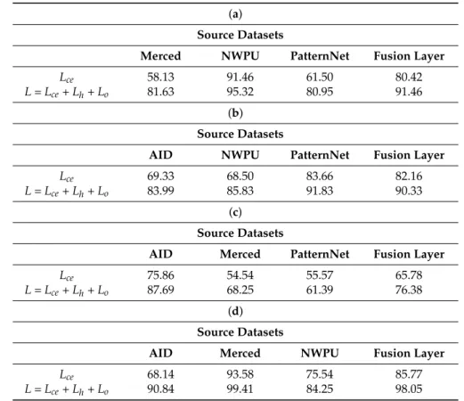
Table2shows the classification accuracies obtained for the four scenarios. In particular, this table shows the accuracy achieved by thek-th branch of the network related to thek-th source dataset in addition to the final accuracy provided by the average fusion layer placed on top of the branches. For the scenario(SMerced,SNWPU,SPatNet)→TAID, we observe that the second branch related to NWPU yields the highest OA, as it is equal to 91.46%, while the other two branches related to Merced and PatternNet yield lower accuracies of 58.13% and 61.50%, respectively. The average fusion layer permits us to obtain the final accuracy of 80.42%. For(SAID,SNWPU,SPatNet)→TMerced, the PatternNet dataset shows a better correlation compared to the other datasets, yeilding an accuracy of 83.66%, while AID and NWPU deliver accuracies of 69.33% and 68.50%, respectively. The fusion layer allows the network to reach an OA of 82.16%. On the other hand, the case (SAID,SMerced,SPatNet)→TNWPU proves to be the more challenging as the branch related to AID results in OA of 75.86%. The other branches related to Merced and PatternNet show weak correlations, as they deliver accuracies of 54.54% and 55.57%, respectively, while the average fusion layer results in an OA of 65.78%. Regarding the last scenario (SAID,SMerced,SNWPU)→TPatNet, we observe that the branch trained on Merced shows a better correlation, as it yields an OA 93.58% compared to the other branches. The average fusion layer of the network permits us to obtain an OA of 85.77%. These preliminary results show that solving only the representation aspect is not sufficient to obtain satisfactory results due to the data-shift problem.

Table 2.Results in terms of overall accuracy (OA) (%) obtained by MB-Net, trained by optimizing the cross-entropy lossLceand the total lossL: (a) AID, (b) Merced, (c) NWPU and (d) PatNet.

(a) Source Datasets

Merced NWPU PatternNet Fusion Layer

Lce 58.13 91.46 61.50 80.42

L=Lce+Lh+Lo 81.63 95.32 80.95 91.46

(b) Source Datasets

AID NWPU PatternNet Fusion Layer

Lce 69.33 68.50 83.66 82.16

L=Lce+Lh+Lo 83.99 85.83 91.83 90.33

(c) Source Datasets

AID Merced PatternNet Fusion Layer

Lce 75.86 54.54 55.57 65.78

L=Lce+Lh+Lo 87.69 68.25 61.39 76.38

(d) Source Datasets

AID Merced NWPU Fusion Layer

Lce 68.14 93.58 75.54 85.77

L=Lce+Lh+Lo 90.84 99.41 84.25 98.05

In the second phase, we optimized MB-Net by adding the losses dealing with the distribution discrepancy between the source and target domains at both representation and decision levels, as explained in the methodology. From Table 2, we observe that the network yields significant improvements in terms of OA for all scenarios. For instance, for (SMerced,SNWPU,SPatNet)→TAID, it gives an accuracy of 91.46% corresponding to an increase of 11%. For the case (SAID,SNWPU,SPatNet)→TMerced, it yields an accuracy of 90.33%, corresponding to an increase of around 8%. Similarly, for (SAID,SMerced,SPatNet)→TNWPU, it reaches an accuracy

(12)

Remote Sens.2018,10, 1890 12 of 18

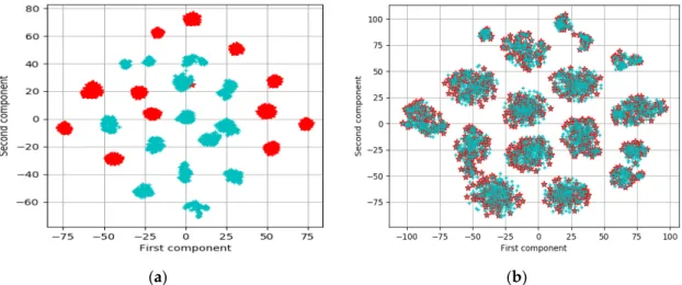
of 76.30% with an increase of around 10%. For the last scenario (SAID,SMerced,SNWPU)→TPatNet, it boosts its accuracy up to 98.05% with of an improvement of 14%. As an indication of the importance of the extra losses related to the domain discrepancy, we provide in Figure8a general view of the distributions in the 2D space of the hidden representation layer with the t-SNE (t-Distributed Stochastic Neighbor Embedding) method [66] for the transfer (SAID,SMerced,SNWPU)→TPatNet. As can be seen, this feature visualization shows an interesting behavior of MB-Net in reducing the distance between the features of the source and target domains before and after adaptation. As additional information related to different object classes, we report in Figures9–12the confusion matrices of all scenarios before and after adaptation. In detail, for the transfer(SMerced,SNWPU,SPatNet)→TAID (Figure9), the MB-Net improves class accuracies by 1% for dense residential, river and sparse residential; 2% for arch-field and anchorage; and 5% for the farm class. For(SAID,SNWPU,SPatNet)→TMerced(Figure10), there is an increase of 1% for anchorage, flyover, and storage cisterns; and 2% for dense residential. Among these classes, the river class seems difficult to classify, although accuracy has been improved by 2%. For(SAID,SMerced,SPatNet)→TNWPU (Figure11), we observe a significant improvement (up to 6%) for the class farm. For the last scenario,(SAID,SMerced,SNWPU)→TPatNet, the network shows a significant improvement for the class farm (up to 7%), while the reaming classes have been improved by 1% and 2%, respectively.

𝐿 = 𝐿 + 𝐿 + 𝐿 81.63 95.32 80.95 91.46 (b)

Source Datasets

AID NWPU PatternNet Fusion Layer

𝐿 69.33 68.50 83.66 82.16

𝐿 = 𝐿 + 𝐿 + 𝐿 83.99 85.83 91.83 90.33 (c)

Source Datasets

AID Merced PatternNet Fusion Layer

𝐿 75.86 54.54 55.57 65.78

𝐿 = 𝐿 + 𝐿 + 𝐿 87.69 68.25 61.39 76.38 (d)

Source Datasets

AID Merced NWPU Fusion Layer

𝐿 68.14 93.58 75.54 85.77

𝐿 = 𝐿 + 𝐿 + 𝐿 90.84 99.41 84.25 98.05

(a) (b)

Figure 8. t-SNE representation of the source and target features obtained at the output of the hidden average layer for the scenario (𝑆 , 𝑆 , 𝑆 ) → 𝑇 when (a) using the 𝐿 loss, and (b) the total loss 𝐿 = 𝐿 + 𝐿 + 𝐿 . (blue: source domain, red: target domain).

Figure 8.t-SNE representation of the source and target features obtained at the output of the hidden average layer for the scenario(SAID,SMerced,SNWPU)→TPatNet when (a) using theLceloss, and (b) the total lossL=Lce+Lh+Lo. (blue: source domain, red: target domain).

(a) (b)

Figure 9. Confusion matrices for AID using: (a) 𝐿 loss, and (b) the total loss 𝐿 = 𝐿 + 𝐿 + 𝐿 .

(a) (b)

Figure 10. Confusion matrices for Merced using: (a) 𝐿 loss, and (b) the total loss 𝐿 = 𝐿 + 𝐿 + 𝐿 .

(a) (b)

Figure 11. Confusion matrices for NWPU using: (a) 𝐿 loss, and (b) the total loss 𝐿 = 𝐿 + 𝐿 + 𝐿 .

(13)

Remote Sens.2018,10, 1890 13 of 18

(a) (b)

Figure 11. Confusion matrices for NWPU using: (a) 𝐿 loss, and (b) the total loss 𝐿 = 𝐿 + 𝐿 + 𝐿 .

Figure 10.Confusion matrices for Merced using: (a)Lceloss, and (b) the total lossL=Lce+Lh+Lo.

(a) (b)

Figure 11.Figure 11. Confusion matrices for NWPU using: (Confusion matrices for NWPU using: (a) a)𝐿 Lce loss, and (loss, and (bb) the total loss) the total loss L𝐿 = 𝐿 + 𝐿 + 𝐿=Lce+Lh+Lo. .

(a) (b)

Figure 12. Confusion matrices for PatternNet using: (a) 𝐿 loss, and (b) the total loss 𝐿 = 𝐿 + 𝐿 +

𝐿 .

4. Discussion

To investigate further the importance of the additional losses 𝐿 and 𝐿 , we repeated the above experiments by considering them independently with the cross-entropy loss 𝐿 . The results depicted in Figure 13 reveal that adding these two losses to 𝐿 permits us to increase the classification accuracy on the unlabeled target data. By averaging the results over the four transfer scenarios, we obtain accuracies of 78.53%, 87.34%, 81.67% and 89.05% for the cases 𝐿 , 𝐿 + 𝐿 , 𝐿 + 𝐿 , and 𝐿 =

𝐿 + 𝐿 + 𝐿 , respectively. We notice that the loss 𝐿 related to the representation level is more relevant than the loss 𝐿 computed at the decision level. Yet, the inclusion of the loss 𝐿 seems reasonable as it can boost further the model accuracy.

Finally, we present in Table 3 a comparison between MB-Net and some recent domain adaptation methods based on a single source. In particular, we compare our results to the adversarial discriminative domain adaptation (ADDA) [49], which combines adversarial and discriminative learning, and the Siamese-GAN method, which reduces the discrepancy between the source and target domains using a Siamese encoder-decoder architecture [59]. These two architectures have been proposed recently for single domain adaptation and they have shown promising results compared to several state-of-the-art methods. Their extension to multisource domain has not been explored yet. To make these methods suitable, we concatenate all sources into one source domain and run the experiments. As can be seen from Table 3, our method provides promising results in terms of classification accuracies. In particular, it provides an average accuracy of 89.05% versus 86.80% and 84.24% for the S-GAN and ADDA methods. Compared to these methods, MB-Net brings the advantage of tackling the domain shift by reducing the discrepancy between the different source domains in addition to the target domain. By contrast, the other approaches mitigate only the difference between a single source and target domains, and ignore the shift between the different sources. The experimental results show the importance of taking into consideration the discrepancy between the different sources and in boosting further the classification accuracy.

Figure 12.Confusion matrices for PatternNet using: (a)Lceloss, and (b) the total lossL=Lce+Lh+Lo.

4. Discussion

To investigate further the importance of the additional lossesLhandLo, we repeated the above experiments by considering them independently with the cross-entropy lossLce. The results depicted

(14)

Remote Sens.2018,10, 1890 14 of 18

in Figure13reveal that adding these two losses toLcepermits us to increase the classification accuracy on the unlabeled target data. By averaging the results over the four transfer scenarios, we obtain accuracies of 78.53%, 87.34%, 81.67% and 89.05% for the casesLce,Lce+Lh,Lce+Lh, andL=Lce+Lh+ Lo, respectively. We notice that the lossLhrelated to the representation level is more relevant than the lossLocomputed at the decision level. Yet, the inclusion of the lossLoseems reasonable as it can boost further the model accuracy.

Figure 13. Sensitivity analysis with respect to the losses 𝐿 , 𝐿 and 𝐿 .

Table 3. Comparisons with respect to state-of-the-art methods.

Target Datasets

Method AID Merced NWPU PatternNet Average Time [m]

ADDA [49] 86.40 85.25 75.22 90.10 84.24 15

S-GAN [59] 88.76 87.30 78.68 92.48 86.80 36

Ours 91.46 90.33 76.38 98.05 89.05 20

5. Conclusions

In this paper we have proposed a multi-branch neural network architecture for tackling the domain adaptation problem from multisource scene datasets. The method optimizes a loss function that reduces the discrepancy between the source and target distributions at the representation and decision levels besides the standard cross-entropy loss. In the experiments, we have validated the method on a multiple source scene dataset built from four scene datasets well known to the remote sensing community. In particular, we have assessed the method using four transfer scenarios (from three source domains to one target domain). The results allow us to draw the following conclusions: (1) deep models based on cross-entropy loss aim to solve the representation aspect; (2) they perform well when source and target domains are from the same domain; (3) they provide reduced accuracies when the distribution of the domains are different; (4) the inclusion of opportune terms in the objective function that reduce the discrepancy between both domains helps reduce this effect; (5) the transfer from multiple sources can further improve accuracy compared to single domain adaptation by handling the multi-domain shifts. For future developments, we plan to propose advanced architectures by taking into consideration the no-shared classes between the different domains. Author Contributions: M.M.A.R. and Y.B. designed and implemented the method, and wrote the paper. T.A., M.L.M., H.A., and M.Z. contributed to the analysis of the experimental results and paper writing.

Funding: This research was funded by the Deanship of Scientific Research at King Saud University through the Local Research Group Program, grant number RG-1435-055.

Acknowledgments: This work was supported by the Deanship of Scientific Research at King Saud University through the Local Research Group Program under Project RG-1435-055.

Conflicts of Interest: The authors declare no conflict of interest.

References

Figure 13.Sensitivity analysis with respect to the lossesLce,LhandLo.

Finally, we present in Table3a comparison between MB-Net and some recent domain adaptation methods based on a single source. In particular, we compare our results to the adversarial discriminative domain adaptation (ADDA) [49], which combines adversarial and discriminative learning, and the Siamese-GAN method, which reduces the discrepancy between the source and target domains using a Siamese encoder-decoder architecture [59]. These two architectures have been proposed recently for single domain adaptation and they have shown promising results compared to several state-of-the-art methods. Their extension to multisource domain has not been explored yet. To make these methods suitable, we concatenate all sources into one source domain and run the experiments. As can be seen from Table3, our method provides promising results in terms of classification accuracies. In particular, it provides an average accuracy of 89.05% versus 86.80% and 84.24% for the S-GAN and ADDA methods. Compared to these methods, MB-Net brings the advantage of tackling the domain shift by reducing the discrepancy between the different source domains in addition to the target domain. By contrast, the other approaches mitigate only the difference between a single source and target domains, and ignore the shift between the different sources. The experimental results show the importance of taking into consideration the discrepancy between the different sources and in boosting further the classification accuracy.

Table 3.Comparisons with respect to state-of-the-art methods.

Target Datasets

Method AID Merced NWPU PatternNet Average Time [m]

ADDA [49] 86.40 85.25 75.22 90.10 84.24 15

S-GAN [59] 88.76 87.30 78.68 92.48 86.80 36

Ours 91.46 90.33 76.38 98.05 89.05 20

5. Conclusions

In this paper we have proposed a multi-branch neural network architecture for tackling the domain adaptation problem from multisource scene datasets. The method optimizes a loss function that reduces the discrepancy between the source and target distributions at the representation and

(15)

Remote Sens.2018,10, 1890 15 of 18

decision levels besides the standard cross-entropy loss. In the experiments, we have validated the method on a multiple source scene dataset built from four scene datasets well known to the remote sensing community. In particular, we have assessed the method using four transfer scenarios (from three source domains to one target domain). The results allow us to draw the following conclusions: (1) deep models based on cross-entropy loss aim to solve the representation aspect; (2) they perform well when source and target domains are from the same domain; (3) they provide reduced accuracies when the distribution of the domains are different; (4) the inclusion of opportune terms in the objective function that reduce the discrepancy between both domains helps reduce this effect; (5) the transfer from multiple sources can further improve accuracy compared to single domain adaptation by handling the multi-domain shifts. For future developments, we plan to propose advanced architectures by taking into consideration the no-shared classes between the different domains.

Author Contributions:M.M.A.R. and Y.B. designed and implemented the method, and wrote the paper. T.A., M.L.M., H.A., and M.Z. contributed to the analysis of the experimental results and paper writing.

Funding:This research was funded by the Deanship of Scientific Research at King Saud University through the Local Research Group Program, grant number RG-1435-055.

Acknowledgments:This work was supported by the Deanship of Scientific Research at King Saud University through the Local Research Group Program under Project RG-1435-055.

Conflicts of Interest:The authors declare no conflict of interest.

References

1. Foody, G.M. Remote sensing of tropical forest environments: Towards the monitoring of environmental resources for sustainable development.Int. J. Remote Sens.2003,24, 4035–4046. [CrossRef]

2. Moranduzzo, T.; Mekhalfi, M.L.; Melgani, F. LBP-based multiclass classification method for UAV imagery. In Proceedings of the 2015 IEEE International Geoscience and Remote Sensing Symposium (IGARSS), Milan, Italy, 26–31 July 2015; pp. 2362–2365.

3. Dean, A.M.; Smith, G.M. An evaluation of per-parcel land cover mapping using maximum likelihood class probabilities.Int. J. Remote Sens.2003,24, 2905–2920. [CrossRef]

4. Myint, S.W.; Gober, P.; Brazel, A.; Grossman-Clarke, S.; Weng, Q. Per-pixel vs. object-based classification of urban land cover extraction using high spatial resolution imagery.Remote Sens. Environ.2011,115, 1145–1161. [CrossRef]

5. Chen, Y.; Zhou, Y.; Ge, Y.; An, R.; Chen, Y. Enhancing Land Cover Mapping through Integration of Pixel-Based and Object-Based Classifications from Remotely Sensed Imagery.Remote Sens.2018,10, 77. [CrossRef] 6. Zhai, D.; Dong, J.; Cadisch, G.; Wang, M.; Kou, W.; Xu, J.; Xiao, X.; Abbas, S. Comparison of Pixel- and

Object-Based Approaches in Phenology-Based Rubber Plantation Mapping in Fragmented Landscapes. Remote Sens.2017,10, 44. [CrossRef]

7. Lopes, M.; Fauvel, M.; Girard, S.; Sheeren, D. Object-based classification of grasslands from high resolution satellite image time series using Gaussian mean map kernels.Remote Sens.2017,9. [CrossRef]

8. Zerrouki, N.; Bouchaffra, D. Pixel-based or Object-based: Which approach is more appropriate for remote sensing image classification? In Proceedings of the 2014 IEEE International Conference on Systems, Man, and Cybernetics (SMC), Qufu, China, 10–12 August 2014; pp. 864–869.

9. Gonçalves, F.M.F.; Guilherme, I.R.; Pedronette, D.C.G. Semantic Guided Interactive Image Retrieval for plant identification.Expert Syst. Appl.2018,91, 12–26. [CrossRef]

10. Demir, B.; Bruzzone, L. A Novel Active Learning Method in Relevance Feedback for Content-Based Remote Sensing Image Retrieval.IEEE Trans. Geosci. Remote Sens.2015,53, 2323–2334. [CrossRef]

11. Zhao, L.J.; Tang, P.; Huo, L.Z. Land-Use Scene Classification Using a Concentric Circle-Structured Multiscale Bag-of-Visual-Words Model.IEEE J. Sel. Top. Appl. Earth Obs. Remote Sens.2014,7, 4620–4631. [CrossRef] 12. Mekhalfi, M.L.; Melgani, F.; Bazi, Y.; Alajlan, N. Land-Use Classification with Compressive Sensing

Multifeature Fusion.IEEE Geosci. Remote Sens. Lett.2015,12, 2155–2159. [CrossRef]

13. Qi, K.; Wu, H.; Shen, C.; Gong, J. Land-Use Scene Classification in High-Resolution Remote Sensing Images Using Improved Correlatons.IEEE Geosci. Remote Sens. Lett.2015,12, 2403–2407. [CrossRef]

(16)

Remote Sens.2018,10, 1890 16 of 18

14. Chen, C.; Zhang, B.; Su, H.; Li, W.; Wang, L. Land-use scene classification using multi-scale completed local binary patterns.Signal Image Video Process.2016,10, 745–752. [CrossRef]

15. Chen, S.; Tian, Y. Pyramid of Spatial Relatons for Scene-Level Land Use Classification.IEEE Trans. Geosci. Remote Sens.2015,53, 1947–1957. [CrossRef]

16. Chen, C.; Zhou, L.; Guo, J.; Li, W.; Su, H.; Guo, F. Gabor-Filtering-Based Completed Local Binary Patterns for Land-Use Scene Classification. In Proceedings of the 2015 IEEE International Conference on Multimedia Big Data, Beijing, China, 20–22 April 2015; pp. 324–329.

17. Zhang, F.; Du, B.; Zhang, L. Scene Classification via a Gradient Boosting Random Convolutional Network Framework.IEEE Trans. Geosci. Remote Sens.2016,54, 1793–1802. [CrossRef]

18. Zhang, L.; Zhang, L.; Du, B. Deep Learning for Remote Sensing Data: A Technical Tutorial on the State of the Art.IEEE Geosci. Remote Sens. Mag.2016,4, 22–40. [CrossRef]

19. Zhang, F.; Du, B.; Zhang, L. Saliency-Guided Unsupervised Feature Learning for Scene Classification. IEEE Trans. Geosci. Remote Sens.2015,53, 2175–2184. [CrossRef]

20. Zou, Q.; Ni, L.; Zhang, T.; Wang, Q. Deep Learning Based Feature Selection for Remote Sensing Scene Classification.IEEE Geosci. Remote Sens. Lett.2015,12, 2321–2325. [CrossRef]

21. Nogueira, K.; Penatti, O.A.B.; dos Santos, J.A. Towards Better Exploiting Convolutional Neural Networks for Remote Sensing Scene Classification.Pattern Recognit.2017,61, 539–556. [CrossRef]

22. Sherrah, J. Fully Convolutional Networks for Dense Semantic Labelling of High-Resolution Aerial Imagery. arXiv2016, arXiv:1606.02585.

23. Lyu, H.; Lu, H. A deep information based transfer learning method to detect annual urban dynamics of Beijing and Newyork from 1984–2016. In Proceedings of the 2017 IEEE International Geoscience and Remote Sensing Symposium (IGARSS), Fort Worth, TX, USA, 23–28 July 2017; pp. 1958–1961.

24. Kendall, A.; Badrinarayanan, V.; Cipolla, R. Bayesian SegNet: Model Uncertainty in Deep Convolutional Encoder-Decoder Architectures for Scene Understanding.arXiv2015, arXiv:1511.02680.

25. Mou, L.; Schmitt, M.; Wang, Y.; Zhu, X.X. A CNN for the identification of corresponding patches in SAR and optical imagery of urban scenes. In Proceedings of the 2017 Joint Urban Remote Sensing Event (JURSE), Dubai, UAE, 6–8 March 2017; pp. 1–4.

26. Cheng, G.; Li, Z.; Yao, X.; Guo, L.; Wei, Z. Remote Sensing Image Scene Classification Using Bag of Convolutional Features.IEEE Geosci. Remote Sens. Lett.2017,14, 1735–1739. [CrossRef]

27. Kussul, N.; Lavreniuk, M.; Skakun, S.; Shelestov, A. Deep Learning Classification of Land Cover and Crop Types Using Remote Sensing Data.IEEE Geosci. Remote Sens. Lett.2017,14, 778–782. [CrossRef]

28. Weng, Q.; Mao, Z.; Lin, J.; Liao, X. Land-use scene classification based on a CNN using a constrained extreme learning machine.Int. J. Remote Sens.2018. [CrossRef]

29. Yu, X.; Wu, X.; Luo, C.; Ren, P. Deep learning in remote sensing scene classification: A data augmentation enhanced convolutional neural network framework.GISci. Remote Sens.2017,54, 741–758. [CrossRef] 30. Sun, S.; Shi, H.; Wu, Y. A survey of multi-source domain adaptation.Inf. Fusion2015,24, 84–92. [CrossRef] 31. Ganin, Y.; Ustinova, E.; Ajakan, H.; Germain, P.; Larochelle, H.; Laviolette, F.; Marchand, M.; Lempitsky, V.

Domain-Adversarial Training of Neural Networks. InDomain Adaptation in Computer Vision Applications; Advances in Computer Vision and Pattern Recognition; Springer: Cham, Switzerland, 2017; pp. 189–209. ISBN 978-3-319-58346-4.

32. Xu, S.; Mu, X.; Chai, D.; Wang, S. Adapting Remote Sensing to New Domain with ELM Parameter Transfer. IEEE Geosci. Remote Sens. Lett.2017,14, 1618–1622. [CrossRef]

33. Ye, M.; Qian, Y.; Zhou, J.; Tang, Y.Y. Dictionary Learning-Based Feature-Level Domain Adaptation for Cross-Scene Hyperspectral Image Classification. IEEE Trans. Geosci. Remote Sens. 2017,55, 1544–1562. [CrossRef]

34. Patel, V.M.; Gopalan, R.; Li, R.; Chellappa, R. Visual Domain Adaptation: A survey of recent advances. IEEE Signal Process. Mag.2015,32, 53–69. [CrossRef]

35. Blitzer, J.; Dredze, M.; Pereira, F. Biographies, Bollywood, Boom-boxes and Blenders: Domain Adaptation for Sentiment Classification. In Proceedings of the ACL 2007—45th Annual Meeting of the Association for Computational Linguistics, Prague, Czech Republic, 23–30 June 2007.

36. Shimodaira, H. Improving predictive inference under covariate shift by weighting the log-likelihood function. J. Stat. Plan. Inference2000,90, 227–244. [CrossRef]

(17)

Remote Sens.2018,10, 1890 17 of 18

37. Sugiyama, M.; Nakajima, S.; Kashima, H.; von Bünau, P.; Kawanabe, M. Direct Importance Estimation with Model Selection and Its Application to Covariate Shift Adaptation. In Proceedings of the Neural Information Processing Systems, Vancouver, BC, Canada, 3–6 December 2007; Volume 20.

38. Duan, L.; Tsang, I.W.; Xu, D.; Maybank, S.J. Domain Transfer SVM for video concept detection. In Proceedings of the 2009 IEEE Conference on Computer Vision and Pattern Recognition, Miami, FL, USA, 20–25 June 2009; pp. 1375–1381.

39. Pan, S.J.; Kwok, J.T.; Yang, Q. Transfer Learning via Dimensionality Reduction. In Proceedings of the 23rd National Conference on Artificial Intelligence, AAAI’08, Chicago, IL, USA, 13–17 July 2008; AAAI Press: Chicago, IL, USA, 2008; Volume 2, pp. 677–682.

40. Long, M.; Wang, J.; Cao, Y.; Sun, J.; Yu, P.S. Deep Learning of Transferable Representation for Scalable Domain Adaptation.IEEE Trans. Knowl. Data Eng.2016,28, 2027–2040. [CrossRef]

41. Ganin, Y.; Lempitsky, V. Unsupervised Domain Adaptation by Backpropagation. In Proceedings of the International Conference on Machine Learning, Lille, France, 6–11 July 2015; pp. 1180–1189.

42. Long, M.; Cao, Y.; Wang, J.; Jordan, M.I. Learning Transferable Features with Deep Adaptation Networks. In Proceedings of the 32nd International Conference on International Conference on Machine Learning, ICML’15, Lille, France, 6–11 July 2015; JMLR.org: Lille, France, 2015; Volume 37, pp. 97–105.

43. Kuzborskij, I.; Maria Carlucci, F.; Caputo, B. When Naive Bayes Nearest Neighbors Meet Convolutional Neural Networks. In Proceedings of the IEEE Conference on Computer Vision and Pattern Recognition, Las Vegas, NV, USA, 27–30 June 2016; pp. 2100–2109.

44. Wang, Y.-X.; Hebert, M. Learning to Learn: Model Regression Networks for Easy Small Sample Learning. In Proceedings of the Computer Vision—ECCV 2016, Amsterdam, The Netherlands, 11–14 October 2016; Lecture Notes in Computer Science. Springer: Cham, Switzerland, 2016; pp. 616–634.

45. Chen, Q.; Huang, J.; Feris, R.; Brown, L.M.; Dong, J.; Yan, S. Deep domain adaptation for describing people based on fine-grained clothing attributes. In Proceedings of the 2015 IEEE Conference on Computer Vision and Pattern Recognition (CVPR), Boston, MA, USA, 7–12 June 2015; pp. 5315–5324.

46. Long, M.; Zhu, H.; Wang, J.; Jordan, M.I. Unsupervised Domain Adaptation with Residual Transfer Networks. arXiv2016, arXiv:1602.04433.

47. Sun, B.; Saenko, K. Deep CORAL: Correlation Alignment for Deep Domain Adaptation. In Proceedings of the Computer Vision, ECCV 2016 Workshops, Amsterdam, The Netherlands, 11–14 October 2016; Lecture Notes in Computer Science; Springer: Cham, Switzerland, 2016; pp. 443–450.

48. Wang, Y.; Li, W.; Dai, D.; Van Gool, L. Deep Domain Adaptation by Geodesic Distance Minimization.arXiv

2017, arXiv:1707.09842.

49. Tzeng, E.; Hoffman, J.; Saenko, K.; Darrell, T. Adversarial Discriminative Domain Adaptation (workshop extended abstract).arXiv2017, arXiv:1702.05464.

50. Luo, P.; Zhuang, F.; Xiong, H.; Xiong, Y.; He, Q. Transfer Learning from Multiple Source Domains via Consensus Regularization. In Proceedings of the 17th ACM Conference on Information and Knowledge Management, CIKM’08, Napa Valley, CA, USA, 26–30 October 2008; ACM: New York, NY, USA, 2008; pp. 103–112.

51. Schweikert, G.; Widmer, C.; Schölkopf, B.; Rätsch, G. An Empirical Analysis of Domain Adaptation Algorithms for Genomic Sequence Analysis. In Proceedings of the 21st International Conference on Neural Information Processing Systems, NIPS’08, Vancouver, BC, Canada, 3–6 December 2007; pp. 1433–1440. 52. Duan, L.; Tsang, I.W.; Xu, D.; Chua, T.-S. Domain Adaptation from Multiple Sources via Auxiliary Classifiers.

In Proceedings of the 26th Annual International Conference on Machine Learning, ICML’09, Montreal, QC, Canada, 14–18 June 2009; ACM: New York, NY, USA, 2009; pp. 289–296.

53. Chattopadhyay, R.; Sun, Q.; Fan, W.; Davidson, I.; Panchanathan, S.; Ye, J. Multisource Domain Adaptation and Its Application to Early Detection of Fatigue.ACM Trans. Knowl. Discov. Data2012,6, 1–26. [CrossRef] 54. Crammer, K.; Kearns, M.; Wortman, J. Learning from Multiple Sources. J. Mach. Learn. Res. 2008, 9,

1757–1774.

55. Hoffman, J.; Kulis, B.; Darrell, T.; Saenko, K. Discovering Latent Domains for Multisource Domain Adaptation. In Proceedings of the Computer Vision—ECCV 2012, Florence, Italy, 7–13 October 2012; Lecture Notes in Computer Science; Springer: Berlin/Heidelberg, Germany, 2012; pp. 702–715, ISBN 978-3-642-33708-6. 56. Kulis, B.; Saenko, K.; Darrell, T. What you saw is not what you get: Domain adaptation using asymmetric

(18)

Remote Sens.2018,10, 1890 18 of 18

57. Duan, L.; Xu, D.; Tsang, I.W.H.; Luo, J. Visual Event Recognition in Videos by Learning from Web Data. IEEE Trans. Pattern Anal. Mach. Intell.2012,34, 1667–1680. [CrossRef] [PubMed]

58. Othman, E.; Bazi, Y.; Melgani, F.; Alhichri, H.; Alajlan, N.; Zuair, M. Domain Adaptation Network for Cross-Scene Classification.IEEE Trans. Geosci. Remote Sens.2017,55, 4441–4456. [CrossRef]

59. Bashmal, L.; Bazi, Y.; AlHichri, H.; AlRahhal, M.; Ammour, N.; Alajlan, N.; Bashmal, L.; Bazi, Y.; AlHichri, H.; AlRahhal, M.M.; et al. Siamese-GAN: Learning Invariant Representations for Aerial Vehicle Image Categorization.Remote Sens.2018,10, 351. [CrossRef]

60. Ammour, N.; Bashmal, L.; Bazi, Y.; Rahhal, M.M.A.; Zuair, M. Asymmetric Adaptation of Deep Features for Cross-Domain Classification in Remote Sensing Imagery.IEEE Geosci. Remote Sens. Lett.2018,15, 597–601. [CrossRef]

61. Yang, Y.; Newsam, S. Bag-of-visual-words and Spatial Extensions for Land-use Classification. In Proceedings of the 18th SIGSPATIAL International Conference on Advances in Geographic Information Systems, GIS’10, San Jose, CA, USA, 3–5 November 2010; ACM: New York, NY, USA, 2010; pp. 270–279.

62. Xia, G.; Hu, J.; Hu, F.; Shi, B.; Bai, X.; Zhong, Y.; Zhang, L.; Lu, X. AID: A Benchmark Data Set for Performance Evaluation of Aerial Scene Classification.IEEE Trans. Geosci. Remote Sens.2017,55, 3965–3981. [CrossRef] 63. Zhou, W.; Newsam, S.; Li, C.; Shao, Z. PatternNet: A benchmark dataset for performance evaluation of

remote sensing image retrieval.ISPRS J. Photogramm. Remote Sens.2018. [CrossRef]

64. Cheng, G.; Han, J.; Lu, X. Remote Sensing Image Scene Classification: Benchmark and State of the Art. Proc. IEEE2017,105, 1865–1883. [CrossRef]

65. He, K.; Zhang, X.; Ren, S.; Sun, J. Deep Residual Learning for Image Recognition. In Proceedings of the 2016 IEEE Conference on Computer Vision and Pattern Recognition (CVPR), Las Vegas, NV, USA, 26 June–1 July 2016; pp. 770–778.

66. van der Maaten, L.; Hinton, G. Visualizing Data using t-SNE.J. Mach. Learn. Res.2008,9, 2579–2605.

© 2018 by the authors. Licensee MDPI, Basel, Switzerland. This article is an open access article distributed under the terms and conditions of the Creative Commons Attribution (CC BY) license (http://creativecommons.org/licenses/by/4.0/).