Duquesne University
Duquesne Scholarship Collection
Electronic Theses and DissertationsFall 2015
Techniques for Estimating the Variance of Specific
Estimators within Complex Surveys
Laura Marie Galiardi
Follow this and additional works at:https://dsc.duq.edu/etd
This Immediate Access is brought to you for free and open access by Duquesne Scholarship Collection. It has been accepted for inclusion in Electronic Theses and Dissertations by an authorized administrator of Duquesne Scholarship Collection. For more information, please contact
Recommended Citation
Galiardi, L. (2015). Techniques for Estimating the Variance of Specific Estimators within Complex Surveys (Master's thesis, Duquesne University). Retrieved fromhttps://dsc.duq.edu/etd/563
TECHNIQUES FOR ESTIMATING THE VARIANCE OF SPECIFIC ESTIMATORS WITHIN COMPLEX SURVEYS
A Thesis
Submitted to the McAnulty College and Graduate School of Liberal Arts
Duquesne University
In partial fulfillment of the requirements for the degree of Master of Science
By Laura Galiardi
Copyright by Laura Galiardi
iii
TECHNIQUES FOR ESTIMATING THE VARIANCE OF SPECIFIC ESTIMATORS WITHIN COMPLEX SURVEYS By Laura Galiardi Approved July29, 2015 ________________________________ Frank D’Amico, Ph.D. Professor of Statistics (Committee Chair) ________________________________ Jeffery Jackson, Ph.D.
Professor of Computer Science Director of Graduate Studies (Committee Member)
_______________________________ John Kern, Ph.D.
Associate Professor of Statistics, Chair (Committee Member)
________________________________ James C. Swindal, Ph.D.
iv
ABSTRACT
TECHNIQUES FOR ESTIMATING THE VARIANCE OF SPECIFIC ESTIMATORS WITHIN COMPLEX SURVEYS
By Laura Galiardi December 2015
Thesis supervised by Dr. Frank D’Amico Professor of Statistics
The objective of this thesis is to present the various procedures for estimating the variance of specific statistics obtained from different types of survey designs, leading up to more advanced designs such complex surveys. The thesis starts with defining the various sampling designs that are to be used for illustrations (Ch 2). Chapter two gives further descriptions of how various sampling designs are performed (from simple designs to not so simple) and shows the sophistication in calculating the estimates and variances. Chapter three cites the actual equations necessary for estimating the variances of the statistics for each design and demonstrates the potential difficulty especially in estimating the variance of the statistics, as the designs get more complex. Each design is illustrated with numerical examples. Chapter four defines current methods for estimating the variance and introduces the Bootstrap and Jackknife approaches. In Chapter 5 the ideas behind what is considered to be a “complex survey” are described and two
v
nationally known complex surveys (NHANES and NHIS) currently being done in the U.S. are explained as examples. Chapter six reports the main statistical results, comparing the variances, etc., for all the designs and finally a summary conclusion is in chapter 7.
vi
DEDICATION
This thesis is dedicated to my family for supporting me through the long, challenging but rewarding journey of my master’s degree, especially my son Jackson who pushed me to
complete this thesis.
In addition, I would like to thank my thesis advisor Dr. D’Amico for working so hard with his busy schedule to make sure I finished.
vii
TABLE OF CONTENTS
Abstract………...………iv
Dedication………...……....vi
Chapter 1: Introduction………..……….1
Chapter 2:Types of Survey Sampling Designs………..……….5
Chapter 3:Numerical Examples Showing the Variance Estimation……….…………14
Chapter 4:Description of current methods used in Variance Estimation……….……….30
Chapter 5: Complex Surveys……….38
Chapter 6: Statistical Results from the Complex Surveys……….45
Chapter 7: Conclusion………56
viii LIST OF TABLES Table 4.1………32 Table 4.2………32 Table 4.3………33 Table 4.4………33 Table 6.1………....46 Table 6.2………46 Table 6.3………47 Table 6.4………47 Table 6.5………49 Table 6.6………51 Table 6.7………54 Table 6.8………55
ix LIST OF FIGURES Figure 2.1……….7 Figure 2.2……….……8 Figure 2.3………...…10 Figure 2.4………...12 Figure 4.1………...36 Figure 4.2………...36
1
Chapter 1 Introduction
Obtaining information and knowledge about human beings has been an issue since civilizations began. Wanting to study human behaviors, emotions, and other pertinent characteristics, man has come up with meaningful ways to “survey” the population. Survey as used in this context implies the simple act of obtaining information from a single individual or collection of individuals. Usually surveys come in the form of a questionnaire that is filled out by someone but it can also be obtained in other ways such as a face-to-face interview, telephone, etc. However, the information obtained is simply accurate to what is collected at that point in time. In the case of health questionnaires, the surveys are called “prevalence” surveys because the statistics calculated from the surveys are prevalence’s of diseases.
Survey design (or methodology) studies the sampling of individual units from a population. Most simple surveys collect data in the form of a questionnaire that is administered to only a random portion of the population, the sample. The answers to the questionnaire are in turn the data that will be statistically analyzed.To ensure the most accurate results the sample should mirror the target population being studied and the survey design(which is how the sampling is to be performed) should not allow for any bias.
In order for a survey to have the most accurate results the sampling method and survey design must follow specific guidelines. Kish (1965)explains,” the sample design has two aspects: a selection process (that is, the rules and operations by which some members of the population are included in the sample); and an estimation process/estimator for computing the sample statistics (which yield the sample estimates of the population values). Different sampling designs would result in different estimates and variances. Choosing the design with the smallest error is the principle aim of sampling design” (Kish, 1965).
2
The true values of the population are known as the parameters. Although for the U.S. Population, they are usually unknown. The estimator or statistic is an estimate computed from
the n elements in the sample. For example, the sample mean (x̅) is the computed mean of then
observations. This particular estimate is only one among the many possible estimates that could
have been obtained from the sampling design.Because the parameters of the population are unknown it is important to understand the variability of the sample estimates. Knowing how the sample estimates can vary helps us to draw conclusions about the parameters. A way of estimating the sampling variability would be to take another sample from the population and compare results. If this was repeated many, many times you would have what is known as the sampling distribution for the statistic. From the distribution of these samples you could determine approximate estimates of the parameters and the variance. This is the asymptotic theory that traditional statistics is based on. However with the recent advances in technology there are other methods (such as “resampling”) being employed for obtaining estimates of the various parameters. Resampling methods treat the sample as if it were itself a population; then we take different samples from this new population and use the subsamples to estimate the variance and other statistics. Bootstrap and Jackknife (Lohr, 1999)are two resampling methods that are currently seen in the literature and there are various software packages that can apply these methods.
Still there are various designs for actually taking the sample. Simple random sample, systematic random sample, stratified, cluster and multi-stage sampling are just some names ofthe methods. Each design has its specific steps depending on what the population looks like. It is easy to assume that all we have to do is reach in and take a suitable sample ofunits from the population. But the units (could be people) are not necessarily nicely defined, even when the
3
population appears to be so. There may be several ways of listing the units, and the size we choose may very well contain smaller subunits. For example suppose we want to find out how many bicycles are owned by residents in a community of 10,000 households. We could just list the households and then take a simple random sample (SRS) of say 400 households or as many as we have estimated we needed. However, maybe the community can be divided into blocks (say 20 households each). The blocks may be grouped geographically for convenience and then randomly sample a certain number of blocks from the listing. Once a block has been selected, then we may either sample all the households within that block or take another random sample of households within each block. This latter plan is an example of cluster sampling. The blocks are the primary sampling units (psus) and the households are the secondary sampling units (ssus).
Bootstrapping is a resampling technique that calculates the variance estimates for a sample in which the Probability Sampling Unitsare sampled with replacement. Another resampling technique that calculates the variance estimates is the Jackknife method, however the Psus are not sampled with replacement in this method.For some clusters such as classrooms, medical practices, or workplaces, it may be just more convenient to sample the entire cluster than to attempt to subsample within the cluster. It is important to know that each method of sampling yields different estimates of the statistics and their variances. Depending on the structure of the sampling some methods may overestimate the variance and result in conservative confidence intervals (Lohr, 1999).
In simple random sampling surveys each observation has the same probability of being chosen. However, there are some cases in which each observation is disproportionately chosen making analysis difficult. Sometimes certain areas of a population may be oversampled, such as what might happen in trying to estimate the health quality of Hispanic or some other group that
4
may not be easily identified for sampling. In which case, we might oversample a particular neighborhood where we know many Hispanics migrate, otherwise in simple random sampling, these individuals would never be selected and our health estimates of the population would be skewed. These cases make up what are known as complex surveys and generally require quite a bit of mathematical adjustment in order to ultimately get unbiased estimates.
Because statistical computing software is now so readily available, resampling techniques have become the standard for computing the variability of various estimators in survey analysis. R is a language and environment for statistical computing and graphics. R is available as Free Software under the terms of the Free Software Foundation's GNU General Public License in source code form. It compiles and runs on a wide variety of UNIX platforms and similar systems including Windows and MacOS. R is an integrated suite of software facilities for data manipulation, calculation and graphical display. Through the online data downloading there are macros written in R that can be used for analyzing survey data for SRS designs thru complex survey designs. And it is free where other computer software for analyzing complex designs, such as SUDAAN, SAS Survey, STATA, and SPSS SVR, all cost a minimum of approximately $1000 or more per yearly license per machine.
5
Chapter 2 Types of Survey Sampling Designs
Simple Random Sampling
“Simple random sampling” (SRS) is a very popular form of probability sampling because of its simplicity in use and analysis. A simple random sample is a subset (a sample) taken from the population. Each item (unit, patient, etc.) in the sample has equal probability of being chosen
from the population (which is𝑁1, N being the number of items in the population). Ideally in small
populations items should not be sampled more than once. Therefore one usually takes a simple random sample without replacement. However the probability of selection in small populations or when a substantial sample size is taken from a larger population can affect the variance estimates. But for the most part, n (sample size) divided by N (population size) is small (less than 5%) and consequently much of the theory in estimating the variance is based on sampling with replacement even though it is not true.
An example may be sampling patients with high blood pressure from hospitals around the county, in order to estimate the rates of various drug medications being used. Suppose there are a total of 1,000 patients with high blood pressure hospitalized in the county. Each patient has a
1
1,000 chance of being chosen if this sampling is done with replacement. If the sampling is done
without replacement then the first patient has a 1,0001 chance. The second patient has a 9991 chance
and the third has 9981 chance of being chosen and so on down the line, until reaching the last
patient who has 100% chance of being sampled. This is impractical because the idea is not to have a sample the same size of the population. Note that usually you start with an estimation process to determine the size of the sample that is necessary to accomplish the analysis. This is
6
then n/N is called the “sampling fraction and abbreviated with the letter “ f. ” The sampling fraction represents what percent of the population needs to be picked. Then depending on the
structure of the population, exactly how we obtain the n units is referred to as the “design”.
Additionally, one other definition that is important in estimating variances is the finite population correction (fpc) factor. It is defined simply as one minus the sampling fraction, in other words,
FPC = 1 –f = 1 – 𝑛𝑁 = 𝑁−𝑛𝑁 .
From this equation, it can be seen that when n is relatively small compared to N, then the fpc is
approximately 100%. Similarly when n is large relative to N, ultimately meaning that a
substantial size of the population is being selected then the fpc plays a larger role in the variance.
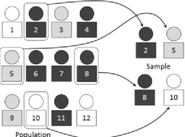
In Figure 2.1, the population size is N = 12 and if n = 4 is chosen a priori, then each
person in the population has a 121 chance being sampled if replacement occurs. Thus the
sampling fraction is 25% and if replacement does not occur then person two (say the first
casedrawn) has a 121 chance of being sampled. Person five (the second case to be selected) has a
1
11 probability of being chosen, while person eight (third selection) has a
1
10 chance, and the
fourthperson (number 10) in the sample had a 19 chance of being selected (Kernler, 2014). If this
7
Figure 2.1. Source: Dan Kernler (2015b), licensed under CC BY SA 4.0
Systematic random sampling
Another form of sampling is systematic sampling; which is performed by arranging the study population according to some ordering scheme and then selecting elements at regular intervals through that ordered list. Systematic sampling involves a random start, known as the
seed, and then proceeds with the selection of every kth element from then onwards. In most cases,
k = 𝑁
𝑛. Usually systematic random sampling is done in multiple passes through the ordered list.
At the outset, each element has an equal probability of being chosen in order to eliminate any bias. For example, suppose there were 1,000 patient visits last year at some clinic and we wish to chart audit a random sample of 50 of them (5%). One could simply obtain the listing of those visits and do a SRS. Or systematically, you could start with the listing and decide you’ll make two passes through the listing. At the end of each pass, you would have chosen about 25 charts from each pass and you would have your 50 cases at the end of two passes. If you were only
8
doing one pass, you would randomly choose a number from 1 to 20 (20 because 1000/50 = k =
20) and then once having that number (say it is the 10th), then you choose the 10th, 30th, 50th, all
the way through the last draw. So the system is choosing every 20th case throughout the listing.
If you wanted to do this in two passes then you would randomly pick a number from 1-40, say
that number is 6, then you sample the 6th, the 46th, the 86th up to the end. That would produce an
approximate sample size of 25. You would then take another random number from 1-40 (now 6 is excluded) and repeat the process to obtain the 50 total cases to be audited.
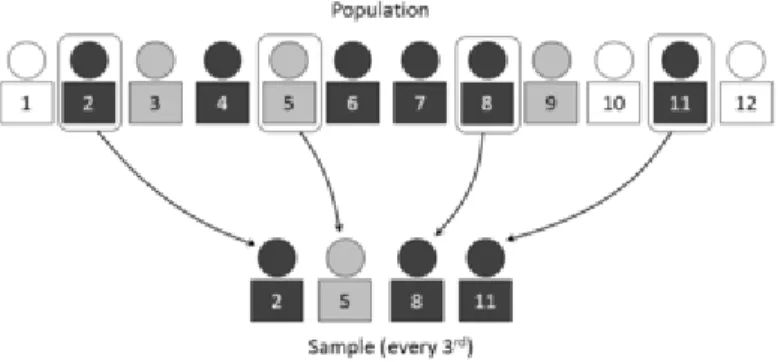
Figure 2.2 shows a simple picture example of a systematic draw where there are twelve people in the population and we need a sample size of four. The seed randomly starts at person two and every third (12/4 = 3) person is sampled. This leaves four people sampled out of the twelve people in the population. As in the previous SRS example, if this were a real problem then the fpc would need to be incorporated in the estimation equations due to its influence on the variance.
9
Stratified Sampling
Stratified sampling is also a type of survey sampling, where the population is organized into a number of distinct categories (called strata). Each stratum is then sampled as an independent sub-population, out of which individual elements can be randomly selected. In order for each element to have an equal probability of being sampled, the stratums must not overlap.
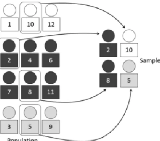
In Figure 2.3, there are three strata of unequal size. Each strata is organized according to color: one white stratum, one black stratum, and one grey stratum. The essential idea is that each strata is considered a subpopulation, usually because of some common attribute; such as race, gender, income, etc. Then within each strata a probability sample is taken proportionate to the
size of the strata relative to the total population. In the example below, we still want n = 4 and
since the black strata has 50% of the population within it, then half of the sample will be
randomly selected from that strata. Thus person ten and five have a 13 chance of being sampled
out of the first and last stratum respectively. Person two has a16 chance while person eight had a 15
probability of being picked, if we are sampling without replacement.
If all the strata were the same size then a SRS would yield on average a sample, which would be representative of the population. However, when strata have varying sizes then independent probability samples must be taken from each strata. Then the overall estimates of the parameters are pooled using one of the various weighting schemes. An example is shown in the next chapter.
10
Figure 2.3. Source: Dan Kernler (2014c), licensed under CC BY SA 4.0
Cluster Sampling
Another form of sampling by groups is called cluster sampling. Stratified and cluster sampling have similarities. They are efficient to use because sometimes it is more cost-effective to select respondents in groups (strata or clusters). But quite often the sampling units are “clustered” by geography, location, density, etc. For instance in surveying households within a city, we might choose to select a certain number of city blocks (for convenience) and then interview every household within the selected blocks. Here the city blocks are the clusters of households. These city blocks can be thought of as strata, but strata usually are different with respect to some other characteristic of the population, such as ethnicity. A certain area of the city comprising different city blocks may be predominantly Hispanic, where other areas may be predominantly white. In order to have representation, the sampling design might first stratify the city by ethnicity and then within each strata would be clusters of city blocks. Then the sampling would take on various stages (multistage sampling).
11
Cluster sampling is commonly implemented as a multistage sampling process. Frongillo (1996) describes a more complex form of cluster sampling. The first stage consists of constructing the clusters that will be sampled (in some cases the clusters to be sampled are chosen for convenience and not selected using probability sampling). In the second stage, a sample of units is randomly selected within each cluster (rather than using all units contained in all selected clusters). In the following stage(s), in each of those selected clusters, random samples of units are selected. All ultimate units (individuals, for instance) selected at the last step of this procedure are then surveyed. This technique is essentially the process of taking random subsamples of preceding random samples. Various national government surveys have this multistage process of selecting individuals from across the U.S. For example, the country is clustered first by density or some other characteristic (such as whether or not that cluster has voted Democratic, etc. in the past) and within each cluster there may be certain strata (defined maybe by median household income). Within these strata, there may be further clusters of the city blocks, etc.
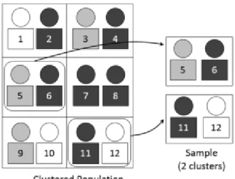
Figure 2.4 shows a simple population of 12 people arranged in six different clusters. Now each of these clusters contains the same number of people, however this is not always the case. Some clusters just like strata can have unequal sizes. The sample in Figure 2.4 contains six clusters and in this design, once a cluster is taken, then every unit within that cluster is in the final sample.
12
Figure 2.4. Source: Dan Kernler (2014a), licensed under CC BY SA 4.0
As mentioned previously, in stratified and cluster the individual sampling elements may not have an equal probability of being sampled. In this case the estimates are usually weighted, if the sample design does not give each individual an equal chance of being selected. For instance, when households have equal selection probabilities but one person is interviewed from within each household, this gives people from large households a smaller chance of being interviewed. This can be accounted for using survey weights. Similarly, households with more than one telephone line have a greater chance of being selected in a random digit dialing sample, and weights can adjust for this. Weights can also serve other purposes, such as helping to correct for non-response.
Complex Survey sampling
In simple surveys each observation has the same probability of being chosen. However, there are some cases in which each observation is disproportionately chosen. In order to have the
13
sample represent the population, information on sampling proportions (called sample weight) is required to properly analyze the survey. In large government national surveys, the sampling process consists of multiple stages of sampling; and at every stage except the last stage, clusters of observations are sampled. At the final stage, the individual observations are sampled. These types of designs where the selection is through a multistage process and in some cases may include “oversampling” in order to obtain reliable estimates are known as “complex surveys”.
A simple example of a complex survey could be where school children are to be sampled. Then the first sampling stage would be to randomly select the schools; then next the classrooms within the schools, and finally the children within classrooms. The first stage of sampling produces what are called the “primary sampling units (PSUs).” This type of sampling is often required because it is logistically impossible, difficult, or expensive to simply try and design a SRS of children directly. The use of multi-stage cluster sampling means that observations cannot be assumed to be independent as is commonly done for a SRS. Observations that are from the same cluster will likely be more similar to each other than to observations from a different cluster (Frongillo, 1996).
14
Chapter 3 Numerical Examples Showing the Variance Estimation
The major goal of sampling is to obtain estimates of population parameters that are as precise as possible, correct and free of bias. We would want to obtain these estimates without actually sampling the entire population and from only sampling small proportions of the population. Since the estimates are based on random samples, they themselves are considered random variables and thus can be described using probability functions. The precision of the estimates while certainly is a function of the sample size, it is also related to the sampling design. As the sample design becomes more intricate, the estimation of the variance also becomes more detailed. This chapter shows examples (Kish, 1965) of how to calculate the variance of the sample mean for each of the designs. In general, the precision of an estimate is often described using 95% confidence intervals (95% CI). The width of the confidence intervals is related to the variance of the estimate. Intervals that are wider show less precision, hence it is important to properly estimate the variance.
Simple Random Sampling
The simple mean of the sample of a SRS selection is the SRS mean, and we distinguish it with the subscript 0;
𝑦0 ̅̅̅ =𝑦 𝑛= 1 𝑛∑ 𝑦𝑗 𝑛 𝑗
Simple random sampling is a sample design specifying both the srs selection and the
simple mean estimate. The variance of the srs mean 𝑦̅̅̅0 is computed as
Var (𝑦̅̅̅ )0 = (1 – f) 𝑠
2
15 Where𝑠2=𝑛−11 ∑ (𝑦𝑗𝑛 𝑗 − 𝑦̅ )2= 𝑛−11 [ ∑ 𝑦𝑗2−𝑦 2 𝑛 𝑛 𝑗 ] = 𝑛 ∑ 𝑦𝑛 𝑗2−𝑦2 𝑛 (𝑛−1 )
The standard error of 𝑦̅̅̅0 is the square root of its variance;
se (𝑦̅̅̅0 ) = √Var (𝑦̅̅̅)0 = √( 1 − 𝑓) 𝑠
√𝑛
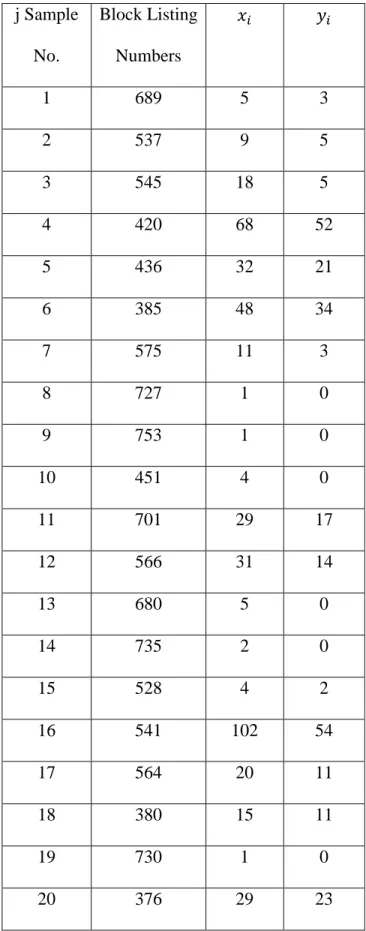
The following SRS (Table 3.1) is from a list of city blocks in Ward 1 in Massachusetts (1950 U.S. Census). The purpose of the survey was to estimate the proportion of dwellings actually owned by the dweller. The actual city blocks are manually arranged in 27 groups of 10
blocks each. The 𝑥𝑖 represents the number of dwellings, and the 𝑦𝑖 denote dwellings occupied by
renters. The population of N = 270 blocks was numbered in the actual problem from 232 to 772 (with block listing numbers that are close together actually representing close proximity to one another within the city). The arranging of the blocks into groups was of 10 was done for convenience. It was estimated that each interviewer could cover about 10-city blocks (or one group) in a day. In this example, with three-digit random numbers, the following SRS of n = 20 was selected. Thus the unit of sampling is the block and in a SRS, every block has an equal
chance of being selected. So n /N =f = 20/270 = .074. This example will be used again (Ch
6) to show the process of estimating the variance for a ratio, such as ( yi / xi ) but this example
shows how to calculate the variance of both X and Y individually. An issue with this design is the number of dwellings within each group is not the same. But according to the sampling design every dwelling within each block is sampled once the group was selected.
16 j Sample No. Block Listing Numbers 𝑥𝑖 𝑦𝑖 1 689 5 3 2 537 9 5 3 545 18 5 4 420 68 52 5 436 32 21 6 385 48 34 7 575 11 3 8 727 1 0 9 753 1 0 10 451 4 0 11 701 29 17 12 566 31 14 13 680 5 0 14 735 2 0 15 528 4 2 16 541 102 54 17 564 20 11 18 380 15 11 19 730 1 0 20 376 29 23
17
The summations of x and y are
∑ 𝑥𝑗 = 435 ∑ 𝑥𝑛 𝑗2 = 22,239 ∑ 𝑦𝑗= 255 ∑ 𝑦𝑛 𝑗2 = 8545
The sample means for the two variances are respectively,
𝑦0 ̅̅̅ = 𝑦 𝑛 = 255 20 = 12.75 and 𝑥̅̅̅0 = 𝑥 𝑛 = 435 20 = 21.75.
The sample variances of the two means are
Var (𝑦̅̅̅ )0 = ( 1 - 20 270 ) 278.62 20 = 12.90 , where 𝑠𝑦 2 = 1 19 [ 8545 - 2552 20 ] = 278.62 , and Var (𝑥̅̅̅ )0 = ( 1 - 27020 ) 672.5120 = 31.14 , where 𝑠𝑥2 = 191 [ 22,239 - 435 2 20 ] = 672.51 ,
and the standard deviations are
𝑠𝑦 = √278.62 = 16.7 and 𝑠𝑥 = √672.51 = 25.9.
The standard errors of the means are
Se (𝑦̅̅̅0) = √12.90 = 3.59 and Se (𝑥̅̅̅0) = √31.14 = 5.58
SYSTEMATIC SAMPLING
There is no design-unbiased variance estimator in systematic sampling(Were, 2015). If we are interested in the true error variance, the only way is to repeat the systematic sample and
18
calculate the variance of all the estimations produced. This is not a viable approach for practical implementation. What is most frequently done for variance estimation of a systematic sample is treating the sample as a simple random sample. However this form of variance estimation consistently over-estimates the true error variance. Numerous approximations have been developed to better estimate the variance of a systematic. One of these methods (successive difference model) is described below. This algorithm was selected due to the relative ease of
implementation(Aune-Lundberg, 2014).
Successive Difference Model (Ordering of Collection Important)
A systematic sample selected with the interval k after a random start yields an equal
probability of being selected because each element has a probability of 1/k being selected. Using this sampling, the sample mean is considered an unbiased estimate of the population mean if the
sample size was fixed at n. If n is not fixed, then the mean is not technically unbiased, but it will
usually be a good estimate. Then the variance equation for this, where g indexes the units of the ordered sample, is given by
Var ( 𝑦̅ ) = 1−𝑓
2𝑛(𝑛−1 )∑ ( 𝑦𝑔 − 𝑦𝑔+1 ) 2. 𝑛−1
𝑔=1
Suppose a systematic sample of n = 40 city blocks out of a population of N = 4000 city blocks results in the following sample, each number represents the number of houses on sampled
block, presented in the order they were drawn:
10, 8, 6, 5, 9, 8, 8, 5, 9, 9, 9, 10, 4, 3, 1, 2, 3, 4, 0, 6,
19
The mean of the sample is 𝑦̅ = 𝑦
𝑛 = 185/40 = 4.625. The variance is given by
Var ( 𝑦̅ ) = 2 𝑥 40 𝑥 390.99 540 = 0.171,
where∑𝑛−1𝑔 ( 𝑦𝑔− 𝑦𝑔+1 )2 = (10 − 8 )2 + ( 8 − 6 )2 + ( 6 − 5 )2 + ( 5 − 9 )2 +………...+
( 1 − 5 )2 + ( 5 − 5 )2 + ( 5 − 4 )2 = 540.
CLUSTER SAMPLING
Clusters of Equal Size
Suppose that from a population of A clusters, a sample clusters are selected with equal
probability. In the selected clusters, all B elements are included in the sample which consists of
a X B = n elements.
The sample mean of the n elements in the sample typically serves to estimate the
population mean. It is also the mean of the 𝑎 cluster means:
𝑦̅= 1𝑛∑ 𝑦𝑛𝑗 𝑗.
The sample size here is fixed at n = a X B. Again the selection of the sample clusters may be systematic, stratified, or even a SRS. For this clustering design, the variance is
Var (𝑦̅) = (1 – f)𝑆𝑎2 𝑎 , where𝑆𝑎 2= 1 𝑎−1∑ (𝑦̅𝛼 𝑎 𝛼 − 𝑦̅)2.
This formula resembles the variance of simple random sampling. In both cases, the variance of the mean is directly proportional to the variance between sampling units and
20
inversely proportional to the number of sampling units. The unit variances are respectively
𝑠2and 𝑠
𝑎2 ; and the sample sizes are, respectively, n and a. Similarly, the cluster sample mean is
the mean of a sampling units selected at random. The variance of the sample mean arises
entirely from variance between the cluster means.
The form 𝑆𝑎2 denotes unit variance between the cluster means 𝑦̅𝛼 . The factor (1-f) becomes negligible for small f, and it disappears for selection with replacement, when clusters are permitted to appear more than once in the sample. But this a theoretical result and sampling with replacement is not usually done in practice.
An example taken from Kish is about a newspaper that has 39,800 subscribers served by carrier routes. There is a card for each subscriber; in a file the cards of each carrier’s route are kept together in geographical order and neighboring routs follow each other. The number of cards per carrier varies between 50 and 200. The chief purpose of the survey is to find out how many of the subscribers own their homes. An interview survey of about 400 subscribers is pre-determined, in small clusters of 10 subscribers each. These save travel time, because an interviewer can generally obtain the 10 interviews in one neighborhood in a short period of time.
The sampler regards the N = 39,800 cards as a frame of A = 3980 clusters of B = 10 each. A few of the clusters will be split between two routes. He selects a = 40 different random numbers, from 1 to 3980. Each random number r denotes the selection of 10 cards numbered from (10r – 9) to 10r; e.g., number 179 will select cards 1781-1790.
The results of the 40 clusters follow (here each cluster has 10 homes within). In terms of
𝑦𝛼 , the data represents the number of homeowners in each cluster of 10 households:
21
3, 5, 0, 3, 0, 0, 4, 0, 8, 0, 10, 5, 6, 1, 3, 3, 1, 5, 5, 4.
So in the first cluster all 10 of the subscribers owned their own home, similarly, in the second cluster 8 out of 10 subscribers owned their own home, and so.
We need to compute only two numbers; y = ∑ 𝑦𝑎 𝛼 = 185; and∑ 𝑦𝑎 𝛼2 = 1263. The
sample mean is simply:
𝑦̅=𝑦𝑛 =185400= 0.4625 = 46.2 percent.
The estimated variance of the sample mean is;
Var (𝑦̅) =1−𝑓𝑎 𝑆𝑎2 = 1−𝑓𝑎 [(𝑎−1 )𝐵1 2( ∑ 𝑦𝛼2−𝑦 2 𝑎 𝑎 𝑎=1 )] = 0.9940[ 39001 (1263 - 185 2 40 )] = 0.9940 (1263−855.6)3900 = 0.99 (.002603) = 0.002585.
The standard error is √0.002585 = 0.05084 = 5.1 percent. The total number of
subscribers who own their own home is estimated as N (𝑦̅ ) 39,000 x 0.4625 = 18,408 = 18,400,
with a standard error of 39,800 x 0.05084 = 2023 = 2000. The 95% confidence interval can be obtained by subtracting and adding two standard errors from the estimated population mean. (18,400 – 4,000 , 18,400 + 4,000) = (14,400 , 22,400)
22
Clusters of Unequal Sizes
Notation for cluster sampling is defined as:
yij = measurement for jth element in the 𝑖th psu
N = number of psus (primary sampling unit sample) in the population
Mi = number of ssus (secondar sampling unit sample) in psu 𝑖
𝑀𝑂 = ∑𝑁 𝑀𝑖
𝑖=1 = total number of ssus in the population
𝑡𝑖 = ∑𝑀𝑗=1𝑖 𝑦𝑖𝑗= total in psui
t = population total
n = number of psus in the sample
𝑚𝑖 = number of ssus in the sample from psui
𝑦̅𝑖 = ∑ 𝑦𝑚𝑖𝑗
𝑖
𝑗 = sample mean (per psu) for psui
𝑡̂𝑖 = ∑ 𝑚𝑀𝑖
𝑖
𝑗 𝑦𝑖𝑗 = estimated total for psui
𝑡𝑢𝑛𝑏̂ = ∑𝑖𝑁𝑛𝑡̂𝑖 = unbiased estimator of population total
𝑆𝑡2 = 𝑛−1 1 ∑ (𝑡𝑖 ̂ −𝑖 𝑡̂𝑢𝑛𝑏𝑁 )2
𝑆𝑖2 = ∑ (𝑦𝑖𝑗−𝑦̅ ) 𝑖
2
𝑚𝑖− 1
𝑗 = sample variance within psui
23
Clusters are rarely of equal size in social surveys. The difference between unequal and
equal-sized clusters is that the variation among the individual cluster totals 𝑡𝑖 is likely to be large
when the clusters have different sizes. The investigators conducting the Enumerative Check
Census of 1937 were interested in the total number of unemployed persons, and 𝑡𝑖 would be the
number of unemployed persons in postal route i. One would expect to find more persons, and
hence more unemployed persons, on a postal route with a large number of households than on a
postal route with a small number of households. So we would expect that 𝑡𝑖 would be large
when the psu size 𝑀𝑖 is large, and small when 𝑀𝑖 is small. Often, then 𝑆𝑖2 is larger in a cluster
sample when the psus have unequal sizes than when the psus all have the same number of ssus.
The probability that a psu is in the sample is n/N, as a srs of n of N psus is taken. Since
one-stage cluster sampling is used, an ssu is included in the sample when its psu is included in the sample. Thus
𝑤𝑖𝑗 = 𝑃(𝑠𝑠𝑢𝑗𝑜𝑓𝑝𝑠𝑢𝑖𝑖𝑠𝑖𝑛𝑠𝑎𝑚𝑝𝑙𝑒)1 = 𝑁𝑛.
One-stage cluster sampling produces a self-weighting sample when the psus are selected with equal probabilities. Using the weights gives us
𝑡𝑢𝑛𝑏̂ = ∑ ∑ 𝑤𝑖 𝑗 𝑖𝑗𝑦𝑖𝑗.
We can use the two formulas above to derive an unbiased estimator for 𝑦̅̅̅̅𝑈 and to find its
standard error. Defined
24
As the total number of ssus in the population; then 𝑌̅̅̅̅̅̅̂𝑢𝑛𝑏 = 𝑡𝑢𝑛𝑏̂ / 𝑀𝑂 and SE (𝑌̅̅̅̅̅̅̂𝑢𝑛𝑏) = SE (𝑡𝑢𝑛𝑏̂ )/
𝑀𝑂. The unbiased estimator of the mean 𝑌̅̅̅̅̅̅̂𝑢𝑛𝑏 can be inefficient when the values of 𝑀𝑖 are
unequal since it, like 𝑡𝑢𝑛𝑏̂ , depends on the variability of the cluster totals 𝑡𝑖. It also requires
the𝑀𝑂be known; however, we often know 𝑀𝑖 only for the sampled clusters. In the Enumerative
Check Census, for example, the number of households on a postal route would only be ascertained for the postal routes actually chosen to be in the sample.
STRATIFIED SAMPLING
The weighted mean and its variance
First we examine the properties of a weighted mean as a general concept. This will allow us to develop later in detail the special formulas appropriate to diverse methods of stratified
sampling. We want to develop a sample estimate for a weighted population mean, 𝑦̅̅̅̅𝑤;
𝑦𝑤
̅̅̅̅=∑ 𝑤ℎ𝑦̅̅̅ℎ = 𝑤1𝑦̅̅̅1 + 𝑤2̅̅̅𝑦2 + . . . + 𝑤ℎ𝑦̅̅̅ℎ + 𝑤𝐻𝑦̅̅̅̅𝐻.
That is, the population mean is equal to the sum of the H strata means 𝑦̅̅̅ℎ , each
multiplied by its proper weight 𝑤ℎ , where ∑ 𝑤ℎ = 1. The weighted sample mean is
𝑦𝑤
̅̅̅̅ = ∑ 𝑤ℎ𝑦̅̅̅ℎ.
The sample mean is obtained separately and independently for each stratum, and it is then multiplied by the weight of the stratum. These products are summed over the H strata to obtain the weighted sample mean. The variance of this weighted mean is obtained by combining the
25
separate variances of the stratum means; The variance of each stratum mean is multiplied by the square of the stratum weight and the products are added over the H strata;
var (𝑦̅̅̅̅ ) = ∑ w𝑤 h2var ( 𝑦̅̅̅ℎ ).
A sample has to be taken in each stratum to estimate its stratum mean, and the sample from each stratum must contain at least two sampling units to permit the computation of the variance in the stratum. The processes of selection and estimation are performed separately and independently within each stratum. Note that nothing was said in this discussion about the sample design within the strata. Thus, within the several strata, different sampling fractions may be used, as well as different methods of selection, estimation and observation.
The sum of the elements contained in all H strata equals the totality of the n elements in the entire population, because each element of the population occurs in one, and only one, stratum;
N =∑ 𝑁ℎ =𝑁1 + N2 + . . . + 𝑁ℎ + . . . + 𝑁𝐻.
The number of elements selected into the sample from the hth stratum is denoted by 𝑛ℎ. The
number of elements in the entire sample is
n = ∑ 𝑛ℎ = 𝑛1+ n2 + . . . + 𝑛ℎ + . . . + 𝑛𝐻.
Typically, 𝑦̅̅̅ℎ is the mean of the 𝑁ℎ elements in the ℎ𝑡ℎ stratum; that is,
𝑦ℎ ̅̅̅ = 𝑁1 ℎ∑ 𝑌ℎ𝑖 𝑁ℎ 𝑖 = 𝑌ℎ 𝑁ℎ ,
Where𝑌ℎ𝑖 is the value of the ithelement in thehthstratum, and 𝑌ℎ is their sum in the hthstratum. The weights frequently, but not always, represent the proportions of the population elements in
26
the strata and 𝑊ℎ = 𝑁ℎ/N. Then the weighted mean is equal to the ordinary mean per element of
the population: 𝑌𝑊 ̅̅̅̅= ∑𝑁ℎ 𝑁= 𝑌̅ℎ= 1 𝑁∑ 𝑌ℎ = 𝑌 𝑁 = 𝑌̅, And then ∑ 𝑊ℎ= ∑𝑁𝑁ℎ= 𝑁1∑ 𝑁ℎ= 𝑁𝑁= 1.
The weight 𝑊ℎ of the stratum is generally, the proportion of the population contained in the
stratum, and so ∑ 𝑊ℎ = 1 . This can be reinforced now by permitting 𝑁ℎ to be any arbitrary
measure of the size of the stratum, no longer restricting it to a count of elements. If we denote
with N = ∑ 𝑁ℎ the sum of these arbitrary measures, 𝑊ℎ = 𝑁ℎ/ N we obtain
𝑌𝑊
̅̅̅̅ = 1
𝑁∑ 𝑁ℎ𝑌̅ .ℎ
and
var ( 𝑌̅̅̅̅𝑊 ) = 𝑁12𝑁ℎ2var (𝑌̅ ).ℎ
We now treat a basic class of stratified samples: those with random selections of elements within each stratum. They are a sample of elements because the elements are selected individually and separately, rather than in clusters. They are stratified because the selection is
carried on separate and independently within each stratum. They are random because the 𝑛ℎ
sample elements are selected with simple random sampling. In this section we present general fundamentals and formulas which can be used for any stratified random sample of elements. They can be used for both disproportionate designs and for proportionate samples. The simple
27 𝑌ℎ0 ̅̅̅̅ = 1 𝑛ℎ∑ 𝑌ℎ𝑖 𝑛ℎ 𝑖
This is the mean of thehth stratum, and selected with simple random sample, as the subscript 0
denotes. For combining the different strata we use the previous mean formula and obtain for the mean of any stratified random sample of elements;
𝑌𝑤0
̅̅̅̅̅ = ∑ 𝑊𝐻 ℎ
ℎ 𝑌̅̅̅̅ℎ0= ∑ 𝑊𝐻ℎ ℎ𝑛1ℎ∑ 𝑌𝑛ℎ𝑖 ℎ𝑖
The variance of the simple random sample of 𝑛ℎ elements in the hth stratum is
Var (𝑌̅̅̅̅ℎ0 ) = ( 1 - 𝑓ℎ ) 𝑆ℎ 2 𝑛ℎ , where 𝑆ℎ 2 = 𝑛1 ℎ−1 ( ∑ 𝑌ℎ𝑖 2 𝑛ℎ 𝑖 - 𝑌ℎ2 𝑛ℎ ).
We combine the variances of the stratum means and obtain the variance of the sample mean 𝑌̅̅̅̅̅𝑤0
as
Var ( 𝑌̅̅̅̅̅𝑤0 ) = ∑ 𝑊ℎ2( 1 - 𝑓ℎ )𝑆ℎ
2
𝑛ℎ
If the weights are based on the proportions of population elements in the strata, then (since 𝑊ℎ =
𝑁ℎ/N and 𝑛ℎ= 𝑓ℎ𝑁ℎ) the above equations can also be expressed, respectively, as
𝑌𝑤0 ̅̅̅̅̅= 1 𝑁∑ 𝑁ℎ 𝐻 ℎ 𝑛1 ℎ∑ 𝑌ℎ𝑖 𝑛ℎ 𝑖 = 1 𝑁∑ 1 𝑓ℎ∑ 𝑌ℎ𝑖 𝑛ℎ 𝑖 𝐻 ℎ Var (𝑌̅̅̅̅̅𝑤0 ) = 𝑁12∑ ( 1 − 𝑓𝐻ℎ ℎ)𝑁ℎ 2 𝑛ℎ 𝑆ℎ 2, where 𝑆ℎ2= 𝑁12∑ 1−𝑓𝑓 ℎ ℎ 𝐻 ℎ 𝑁ℎ𝑆ℎ2.
If the 𝑌̅̅̅̅̅𝑤0 denotes a proportion 𝑃𝑤0 = ∑ 𝑊ℎ𝑃ℎits variance may be written in an equivalent form
28
Var(𝑃𝑤0 ) = ∑ 𝑊ℎ2 ( 1 - 𝑓ℎ ) 𝑃ℎ ( 1−𝑃ℎ )𝑛
ℎ− 1 .
For a numerical illustration and using the data from Table 3.2,suppose we select a sample of n = 400 employees out of N = 10,000 employed in a factory. We use the several departments of the factory as strata, because it can be done easily, and because we suspect that there may be large differences in the employee’s responses among the departments for the survey variables.
Symbol Assembly Foundry and
Machine
Office and Miscellaneous
Entire Factory
Stratum Number h 1 2 3 Total
Population Size 𝑁ℎ 5000 3010 1990 10,000 Stratum Weight 𝑊ℎ 0.50 0.30 0.20 1.00 Sample Size 𝑛ℎ 200 120 80 400 Number of “yes” answers 𝑦ℎ 14 18 48 80 The percentage of “yes” answers 𝑦ℎ ̅̅̅ 7% 15% 60% 20 Table 3.2 𝑃𝑤0 = ∑ 𝑊ℎ𝑌̅̅̅̅ℎ𝑜 = 0.50(7) + 0.30(15) + 0.20(60) = 20 percent
29
Var(𝑃𝑤0) = [0.502 24257 (93)199 + 0.302 242515(85)119 + 0.202 242560(40)79 ] x 0.001
= 0.000288
The standard error of the 𝑃𝑤 = 0.20 is
30
Chapter 4 Description of current methods used in Variance Estimation
For the purpose of this thesis Jackknife and Bootstrap are two resampling techniques that were used to verify the precision of the sample statistics (mean, median, variance, and percentile) computed for data sets. Later a comparison of the two techniques will examine if Bootstrap or Jackknife was more accurate at estimating such statistics. Bootstrap and Jackknife execute two different methods to establish estimates but both techniques develop large amounts of subsamples from the sample. Lohr explains how, resampling methods treat the sample as if it were itself a population: they take different samples from this new “population” and use the subsamples to estimate the variance.” There are several resampling techniques available but his paper will focus on the Bootstrapping and Jackknife methods.
The use of high powered computer software has made the Jackknife and Bootstrap procedures very popular. Shao and Tu further describe the frequent use of both methods, “The jackknife and bootstrap are the most popular data-resampling methods used in statistical analysis. These resampling methods replace theoretical derivations required in applying traditional methods (such as substitution and linearization) in statistical analysis by repeatedly resampling the original data and making inferences from the resamples. Because of the availability of inexpensive and fast computing software, these computer-intensive methods have caught on very rapidly in recent years and are particularly appreciated by applied statisticians.”
The Jackknife method was introduced by Quenouille in 1956. Quenouille’s original purpose for the Jackknife was to reduce the bias of sample estimates. It was not until 1958 when Tukey proposed using it to estimate variances and calculate confidence intervals. The jackknife estimator of a parameter is found by systematically leaving out each observation from a dataset
31
and calculating the estimate based on the rest of the observations and then finding the average of these calculations. Each data point goes through the process of being deleted. If one observation is deleted at a time then a sample of 1,000 will have 1,000 subsample of the sample. Therefore every time Jackknife is run on a data set the exact same result will occur.
Some advantages of the Jackknife include working for multistage samples in which other resampling techniques do not. As mentioned previously, it provides a consistent estimator of the mean and variance and tends to be asymptotically true (Rao and Shao, 1992). However the Jackknife method requires intensive computation that must be done with computer software. Most data sets are too large and time consuming for hand calculation and require running computer programs. Furthermore, this method assumes independence between the random variables (and identically distributed data points), and if that assumption is violated, the results will be of no use. Thus the variables must be independent from each other for the Jackknife estimates to be accurate.
Using the cluster example from chapter 3, I will demonstrate how R can generate Jackknife estimates of the mean and variance of the 39,000 newspaper subscribers. Table 4.1 contains the R code for the first few steps of the Jackknife example. The bootstrap package in R
was installed for analysis. The first step is to input the data named ownhome and call the
32 INPUT ownhome<-c(10, 8, 6, 5, 9, 8, 8, 5, 9, 9, 9, 10, 4, 3, 1, 2, 3, 4, 0, 6, 3, 5, 0, 3, 0, 0, 4, 0, 8, 0, 10, 5, 6, 1, 3, 3, 1, 5, 5, 4) library(bootstrap) Table 4.1
The following code in table 4.2 jackknifes the sum of the forty clusters. Forty subsamples were generated because one cluster was deleted at a time and then the rest of the data was totaled. This process was written as a function called theta, the results of the function are jackknifed and the vector of subsamples are called results$jack.values. The mean of results$jack.values is 180.375. INPUT OUTPUT theta<-function(ownhome){sum(ownhome)} results<-jackknife(ownhome,theta) results$jack.values [1] 175 177 179 180 176 177 177 180 176 176 175 181 182 184 183 182 181 185 179 [20] 182 180 185 182 185 185 181 185 177 185 175 180 179 184 182 182 184 180 180 [39] 181 176 mean(results$jack.values) [1] 180.375 Table 4.2
33
Finding the sample mean is done by taking
𝑦̅ = 𝑦
𝑛 = 180.375
400 = 0.4509 = 45 percent.
The estimated variance of the sample mean
Var (𝑦̅) = 1−𝑓 𝑎 𝑆𝑎 2 = 1−𝑓 𝑎 [ 1 (𝑎−1 )𝐵2 ( ∑ 𝑦𝛼2− 𝑦2 𝑎 𝑎 )] = 0.9940[ 39001 (1263 – 180.375 2 40 )] = 0.9940 (1263−813.37)3900 = 0.02475 (.11539) = 0.002855.
The standard error is √0.002855 = 0.05344 = 5.3 percent. The total number of
subscribers who own their own home is estimated as N(𝑦̅ ) 39,800 x 0.4509 = 17,945 with a
standard error of 39,800 x 0.05344 = 2127. The 95% confidence interval can be obtained by subtracting and adding two standard errors from the estimated population mean. (17,945 – 4,254
, 17,945 + 4,254) = (13,691 , 22,199).
Bootstrap is the other resampling technique utilized in this research. The Bootstrap is a method of resampling with replacement where as the Jackknife is a resampling method without replacement. It was introduced as a spinoff of the Jackknife by Bradley Efron in 1979. The
bootstrap subsamples are pulled from the sample of sizen. Assuming that n is sufficiently large
there is zero probability the resamples are identical to the original sample. The sampling processes is repeated a large number of times e.g. 10,000. For each of the bootstrap samples the mean is calculated (or any estimator) and called the bootstrap estimates. We now have 10,000
34
subsamples of the sample mean and can make a histogram of bootstrap means. This provides an estimate of the shape of the distribution of the mean from which we can answer questions about how much the mean varies. The method here, described for the mean, can be applied to almost any other statistic or estimator (median, percentile, or variance).
The popularity of the bootstrap method is attributed to its simplicity to derive estimates for complex data sets. Bootstrap is also an appropriate way to control and check the stability of the results. Histograms and other plots provide much information as to the variability of each statistic. For most problems it is impossible to know the true confidence interval, bootstrap is asymptotically more accurate than the standard intervals obtained using sample variance. In some conditions bootstrapping is asymptotically consistent, but it does not provide general finite-sample guarantees. The apparent simplicity may conceal the fact that important assumptions are being made when undertaking the bootstrap analysis. Similar to the Jackknife method the Bootstrap assumes data independence.
Once again using the newspaper subscriber example from Chapter 3, R will be used to compile bootstrap estimates to find the variance of the sample mean. Table 4.3 shows the steps needed for bootstrap analysis and is similar to the Jackknife code. The first step is to input the
data named ownhome. Then a function called samplesum was written that returns the sum of the
35 INPUT ownhome<-c(10, 8, 6, 5, 9, 8, 8, 5, 9, 9, 10, 4, 3, 1, 2, 3, 4, 0, 6, 3, 5, 0, 3, 0, 0, 4, 0, 8, 0, 10, 5, 6, 1, 3, 3, 1, 5, 5, 4, 9) samplesum<- function(ownhome,i) { d2 <- ownhome[i] return(sum(d2)) } b = boot(ownhome, samplesum, R=1000) Table 4.3
The mean of the 1,000 subsamples is found by calling b, which is shown in table 4.4 as 185.46
INPUT OUTPUT
b Bootstrap Statistics :
original bias std. error t1* 185 0.462 20.90807
mean(b$t) [1] 185.462
Table 4.4
Below in figure 4.1 and 4.2 is a histogram and normal quantile plot of the 1,000 bootstrap samples. The dotted line at 185.46 in the center of the histogram is the mean of the 1,000 bootstrap samples.
36
Figure4.1 Figure 4.2
Finding the sample mean is done by taking
𝑦̅ = 𝑦𝑛 = 185.462400 = 0.4635 = 46.35 percent.
The estimated variance of the sample mean is:
Var(𝑦̅) = 1−𝑓𝑎 𝑆𝑎2 = 1−𝑓𝑎 [ 1 (𝑎−1 )𝐵2 ( ∑ 𝑦𝛼2− 𝑦2 𝑎 𝑎 )] = 0.9940[ 39001 (1263 – 185.462 2 40 )] = 0.9940 (1263−859.9038)3900 = 0.02475 (.103358) = 0.002558.
37
The standard error is √0.002558 = 0.05057 = 5.05 percent. The total number of
subscribers who own their own home is estimated as N(𝑦̅ ) 39,800 x 0.4635 = 18,560 with a
standard error of 39,800 x 0.05057 = 2012. The 95% confidence interval can be obtained bysubtracting and adding two standard errors from the estimated population mean. (18,560 –
38
Chapter5 Complex Surveys
Most large surveys involve several of the concepts previously mentioned. The survey may be stratified with several stages of clustering and quite often employs multiple probability schemes in order to obtain samples that are “rich” in information. Further information on sampling proportions called sample weights is required in order to properly analyze a survey of this nature. Often the analysis relies on various levels of regression estimations. Surveys combining the components of random sampling, stratification, clustering, and sophisticated regression type analyses are referred to as “complex surveys”.
Complex surveys have multiple stages of sampling. At every stage except the lowest stage, clusters of observations are sampled. At the lowest stage, the individual observations are sampled. Frongillo gives an example: a survey of school children may be collected by first sampling the schools within some region; then sample the classrooms within each school and finally sample the children within those classrooms. This type of sampling is often required because it is logistically impossible, difficult, or expensive to sample the students directly. The formulas for estimating the standard errors are complicated and require specialized computer intensive software packages.
There are many datasets obtained from various complex surveys that are available online. All contain various de-identified information on the subjects. In order that subjects cannot be identified, variables such as age are recoded into categories; similarly rather than give a subject’s address, their city or county may be recoded and only those codes are given in the survey. Depending on the purpose of the survey, sensitive information is not downloadable but may be obtained from the survey collection agencies with specific IRB approval.
39
The U.S. government spends millions of dollars each year collecting survey data from the U.S. population. These datasets are organized coded files that can be obtained with specific statistical software. They are freely available and can be downloaded from the web. While each survey has its objectives, the government collects this data with really no primary purpose. Their intention is for researchers to have access to population data for getting answers to health related questions that the investigator has come up with. Consequently these datasets are referred to as “secondary data files.” To see the multitude of data and listings of these files, all one has to do is to Google www.cdc.gov/nchs. All files are identified by their acronym name such as NHIS (National Health Interview Survey), NSFG (National Survey of Family Growth), NHANES (National Health and Nutritional Exam Survey), NHDS (National Hospital Discharge Survey), etc. Many of these surveys are performed yearly. The NHIS is the major survey that the government uses to obtain information on the health of the population and study changes from year to year. The NHANES survey is an extensive survey to estimate what the population is eating, their exercise and disease prevalence and other areas as well. A short description of two surveys (NHIS and NHANES) follows.
NHIS (National Health Interview Survey)
The National Health Interview Survey (NHIS) provides vital information on the health of the civilian noninstitutionalized population of the United States and is one of the major data collection programs of the National Center for Health Statistics (NCHS) which is part of the Centers for Disease Control and Prevention (CDC). NHIS data are used widely throughout the Department of Health and Human Services (DHHS) to monitor trends in illness and disability and to track progress toward achieving national health objectives. The data are also used by the
40
public health research community for epidemiologic and policy analysis of such timely issues as characterizing those with various health problems, determining barriers to accessing and using appropriate health care, and evaluating Federal health programs.
The National Health Interview Survey is a cross-sectional household interview survey. Sampling and interviewing are continuous throughout each year. The sampling plan follows a multistage area probability design that permits the representative sampling of households and noninstitutional group quarters (e.g., college dormitories). The sampling plan is redesigned after every decennial census. The first stage of the current sampling plan consists of a sample of 428 primary sampling units (PSU's) drawn from approximately 1,900 geographically defined PSU's that cover the 50 States and the District of Columbia. A PSU consists of a county, a small group of contiguous counties, or a metropolitan statistical area.
Within a PSU, two types of second-stage units are used: area segments and permit segments. Area segments are defined geographically and contain an expected eight, twelve, or sixteen addresses. Permit segments cover housing units built after the 2000 census. The permit segments are defined using updated lists of building permits issued in the PSU since 2000 and contain an expected four addresses. The NHIS sample is drawn from each State and the District of Columbia. The total NHIS sample is subdivided into four separate panels, or subdesigns, such that each panel is a representative sample of the U.S. population. The expected NHIS sample size (completed interviews) is approximately 35,000 households containing about 87,500 persons. The annual response rate of NHIS is close to 90 percent of the eligible households in the sample.
Data are collected through a personal household interview conducted by interviewers employed and trained by the U.S. Bureau of the Census according to procedures specified by the
41
NCHS. For the Family Core component, all adult members of the household 17 years of age and over who are at home at the time of the interview are invited to participate and to respond for themselves. For children and for adults not at home during the interview, information can be provided by a responsible adult family member, 18 years of age and over, residing in the household.
NHANES (National Health and Nutritional Exam Survey)
The two complex surveys utilized in this thesis are the National Health Interview Survey from 2012 (NHANES 2012) and the National Health Interview Survey II (NHANES II). This survey is one of the major data collection programs of the National Center for Health Statistics (NCHS) which is part of the Centers for Disease Control and Prevention (CDC). NHANES is arguably the largest and longest-running national source of objectively measured health and nutrition data. The survey is unique in that it combines interviews and physical examinations to collect data. Through the physical examinations, clinical and laboratory tests, and personal interviews, NHANES provides a "snapshot" of the health and nutritional status of the U.S. population. Findings from NHANES provide health professionals and policymakers with the statistical data needed to determine rates of major diseases and health conditions (e.g., cardiovascular disease, diabetes, obesity, infectious diseases) as well as identify and monitor trends in medical conditions, risk factors, and emerging public health issues, so that the appropriate public health policies and prevention interventions can be developed.
Five NHANES have been conducted since 1970. NHANES I, the first cycle of the NHANES studies, was conducted between 1971 and 1975 and included a national sample of
42
approximately 30,000 individuals between one and seventy-four years of age. NHANES II (1976–1980) included just slightly over 25,000 participants and expanded the age of the first NHANES sample somewhat by including individuals as young as 6 months of age. In addition, children and adults living at or below the poverty level were sampled at higher rates than their proportions in the general population ("oversampled") because these individuals were thought to be at particular nutritional risk.
The second National Health and Nutrition Examination Survey, NHANES II, is a nationwide probability sample of 27,801 persons from 6 months to 74 years of age. From this sample, 25,286 people were interviewed and 20,322 people were examined, resulting in an overall response rate of 73 percent. Because children and persons classified as living at or below the poverty level were assumed to be at special risk of having nutritional problems, they were sampled at rates substantially higher than their proportions in the general population. Adjusted sampling weights were computed within 76 age-sex income groups in order to inflate the sample to closely reflect the target population at the midpoint of the survey.
Beginning in 1999, NHANES became a "continuous survey." That is, unlike the previous NHANES surveys, which were conducted over a period of approximately four years with a "break" of at least one year between survey periods, the 1999–2000 survey was (and all subsequent surveys will be) conducted without breaks, on a yearly basis. As the survey period is shorter in length, the subject sample will be smaller. The 1999–2000 survey included nutritional and medical data on approximately 8,837 individuals up to 74 years of age.
In current practice, however, NHANES data are derived primarily from the first two sources; that is, via direct interview and direct clinical examination. The NHANES data collection procedures have changed slightly over the years. These changes reflect not only the
43
changing demographics of the United States over time, but also the changing nature of the survey (e.g., the inclusion of the nutrition component, the interest in the effects of environment upon health). Nonetheless, the basic trends of data collection, particularly with regards to sampling, are similar.
The primary sample design change for NHANES 2011-2012 is that there is an oversample of Non-Hispanic Asians in addition to the ongoing oversample of Hispanics, non-Hispanic Blacks, older adults, and low income whites/others. Since the total sample size in any year is fixed due to operational constraints, sample sizes for Hispanic persons and non-low income white and other persons were decreased in order to increase the sample sizes for Asians. Consequently, sample sizes for Mexican American Hispanic persons were also decreased compared to survey cycles prior to 2011.
NHANES uses a complex, multistage probability design to sample the civilian, noninstitutionalized population residing in the 50 states and D.C. Sample selection for NHANES followed these stages, in order:
1. Selection of primary sampling units (PSUs), which are counties or small groups
of contiguous counties.
2. Selection of segments within PSUs that constitute a block or group of blocks
containing a cluster of households.
3. Selection of specific households within segments.