A penalized framework for distributed lag non-linear models.

(1)

ISSN 0006-341X DOI: https://doi.org/10.1111/biom.12645 Downloaded from: http://researchonline.lshtm.ac.uk/3429699/ DOI:10.1111/biom.12645

Usage Guidelines

Please refer to usage guidelines at http://researchonline.lshtm.ac.uk/policies.html or

alterna-tively [email protected].

(2)

A Penalized Framework for Distributed Lag Non-Linear Models

Antonio Gasparrini,1,2,* Fabian Scheipl,3 _{Ben Armstrong,}1 _{and Michael G. Kenward}2

1_{Department of Social and Environmental Health Research, London School of Hygiene & Tropical Medicine,} 15–17 Tavistock Place, London WC1H 9SH, U.K.

2_{Department of Medical Statistics, London School of Hygiene & Tropical Medicine, Keppel Street,} London WC1E 7HT, U.K.

3_{Department of Statistics, Ludwig Maximilians University, Munich, Germany} ∗_email:_{[email protected]}

Summary. Distributed lag non-linear models (DLNMs) are a modelling tool for describing potentially non-linear and delayed dependencies. Here, we illustrate an extension of the DLNM framework through the use of penalized splines within generalized additive models (GAM). This extension offers built-in model selection procedures and the possibility of accommodating assumptions on the shape of the lag structure through specific penalties. In addition, this framework includes, as special cases, simpler models previously proposed for linear relationships (DLMs). Alternative versions of penalized DLNMs are compared with each other and with the standard unpenalized version in a simulation study. Results show that this penalized extension to the DLNM class provides greater flexibility and improved inferential properties. The framework exploits recent theoretical developments of GAMs and is implemented using efficient routines within freely available software. Real-data applications are illustrated through two reproducible examples in time series and survival analysis.

Key words: _{Distributed lag; Exposure-lag-response; Generalized additive models; Latency; Penalized splines.}

1. Introduction

Distributed lag models (DLMs), originally proposed in econo-metrics by Almon (1965) and more recently in epidemiology by Schwartz (2000), constitute an elegant analytical frame-work to describe associations characterized by a delay between an input and a response in time series data. DLMs model the response yt observed at time t in terms of past

occur-rences xt− of a predictor x. The new quantity , the lag, defines a new space that expresses the temporal structure of the association. In standard DLMs, a parametric function is applied to model the shape of the lag structure, usually polynomials or less often regression splines. However, the esti-mated shape is dependent on the chosen parametric form, for instance, the degree of the polynomial or the number and locations of the splines knots. More sophisticated smooth-ing techniques have been proposed to address this issue in DLMs, including penalized splines through generalized addi-tive models (GAMs) (Zanobetti et al., 2000; Muggeo, 2008; Rushworth et al., 2013; Obermeier et al., 2015) or Bayesian approaches with the definition of prior distributions (Welty et al., 2009). While these methods offer greater flexibility and more advanced model selection procedures, they rely on the strong assumption of a linear or linear-threshold dose-response relationship, and are only applicable to time series data.

Recent work has addressed these limitations. First, Armstrong (2006) and Gasparrini et al. (2010) extended DLMs to distributed lag non-linear models (DLNMs), a framework to describe bi-dimensionaldose-lag-response asso-ciations potentially varying non-linearly in the dimensions of

predictor intensity and lag. Second, Gasparrini (2014) gen-eralized DLMs and DLNMs beyond the time series setting, extending their application to other designs and data struc-tures. However, the current version of DLNMs still requires the user to select the parametric form of the functions expressing the dose-lag-response relationship. Model selection procedures based on information criteria have been proposed, but they lack a solid theoretical basis, and have been shown to partly aﬀect the inferential properties of the estimators (Gasparrini, 2014; Obermeier et al., 2015).

In this contribution, we propose an extended DLNM class developed through penalized splines regression. This devel-opment provides greater flexibility for modelling potentially complex bi-dimensional dose-lag-response relationships, and offers built-in model selection and inferential procedures based on recent theoretical work on GAMs. In addition, we extend the methodology further to accommodate a pri-ori assumptions on the shape of the lag structure through the definition of specific penalties. This general framework is applicable to model either linear or non-linear lagged rela-tionships, in various study designs based on either time series or other data structures, and includes most of the models described above as special cases. This extension is fully imple-mented in freely available software routines.

The article is structured as follows: Section 2 brieﬂy revisits the deﬁnition of DLNMs. Section 3 illustrates the extension to a penalized version of DLNMs. In Section 4, we present a simulation study for the assessment of the performance and inferential properties of both standard and extended versions. In Section 5, penalized DLNM are applied in two reproducible

©2017 The AuthorsBiometricspublished by Wiley Periodicals, Inc. on behalf of International Biometric Society This is an open access article under the terms of the Creative Commons Attribution License, which permits use, distribution and reproduction in any medium, provided the original work is properly cited.

(3)

illustrative examples. A ﬁnal discussion is provided in Sec-tion 6. AddiSec-tional informaSec-tion and results are provided in the Web material.

2. The DLNM Framework

In time series data, DLMs and DLNMs model a response

yt measured at time t=1, . . . , m in terms of lagged

occur-rences of a predictor xt, represented by the vector qt =

[xt−0, . . . , xt−L]

T_{, with}

0 and L as minimum and maximum

lags, respectively, (Gasparrini et al., 2010). The framework can be extended beyond the time series setting by including an additional indexing structure, allowing each response yi,t,

withi=1, . . . , n, to depend on equally spaced lagged values

qi,t=[xi,t−0, . . . , xi,t−L]

T_{. Here, each observation identified by} the index i, for instance, a specific subject followed in time, refers to a differentexposure profilethat determines the lagged dose pattern at time t. Time series data represent a special case where i=t, while extensions to more complex designs such as survival or repeated-measures longitudinal data are straightforward. See Gasparrini (2014) for a more detailed explanation of the extension beyond time series data and related algebraic definitions.

The association is represented through a functions, deﬁned as:

s(qi,t)=s(xi,t−0, . . . , xi,t−L)=

L =0

f·w(xi,t−, ). (1)

Here, the bi-dimensional dose-lag-response function f· w(x, ) is composed of two marginal functions: the standard dose-response functionf(x), and the additional lag-response function w() that models the lag structure in the space =[0, . . . , L]T. Parameterization off andwis obtained by

applying known basis transformations to the vectorsqi,tand, producing marginal basis matricesRi,tandCwith dimensions (L−0+1)×vx and (L−0+1)×v, respectively.

Identi-ﬁability constraints require a reparameterization of R (see Section 3.2). The functions, here termedcross-basisfunction and parameterized by coeﬃcientsη, is constructed by:

s(xi,t−0, . . . , xi,t−L;η)=(1

T

L−0+1Ai,t)η=w

T

i,tη, (2)

withwi,tas a set of known transformations derived fromAi,t, which in turn is computed by a row-wise Kronecker product between the two basis matrices (Eilers et al., 2006), as:

Ai,t=(Ri,t⊗1T_v)(1T_v_x⊗C), (3) with1jas a vector of 1’s with lengthj. Then×vx·v

cross-basis matrixW, obtained by applying (1)–(3) to the full set of n observations, can be included in the design matrix of standard regression models, such as generalized linear models (GLMs) or Cox proportional hazard models, to estimate the parametersη.

The dose-lag-response surface can be recovered by predict-ing eﬀects ˆβx, on a grid of predictor valuesxand lag . For

ease of interpretation, ˆβx, are deﬁned as speciﬁc contrasts

of f·w(x, ) by centering the dose-response function f(x) to

a reference value of the predictor x. These eﬀects ˆβx, are

interpreted in the usual scale of risk ratio or diﬀerence. In par-ticular, the analysis commonly focuses on speciﬁc summaries, such as estimated lag-response associations at a given predic-tor value, or the overall dose-response association obtained by cumulating the risk across the lag period. Algebraic and interpretational details are given elsewhere (Armstrong, 2006; Gasparrini et al., 2010; Gasparrini, 2014).

3. Penalized DLNMs

A penalized extension of DLNM can be described within the family of GAMs (Hastie and Tibshirani, 1990; Wood, 2006a). These models extend the strong parametric form of GLMs by allowing the linear predictor to include flexible smooth func-tions of the covariates. A recent development of GAMs defines smooth components through penalized regression splines, using low-rank basis terms and a simple form of penalized likelihood (Wood, 2006b). This definition provides theoret-ically well-grounded estimators implemented using efficient and numerically stable routines (Wood, 2008, 2011). We refer to the two versions of the method as unpenalized and penalized DLNMs, sometimes using the shortcuts GLMs and GAMs, respectively.

3.1. Penalized Likelihood

In unpenalized models, the dose-lag-response association defined by a DLNM can be estimated by maximizing the model likelihood l(η,γ) in terms of the model parameters [ηT_,_γT_]T_{, with} _η _{corresponding to coefficients of the} cross-basis and γ to coefficients of additional covariate terms in the model, respectively. The idea underlying the extension to penalized DLNM is to form a richly parameterized cross-basis, and then to apply penalties through its parametersηto smooth the dose-lag-response surface. Following similar devel-opments for tensor product bi-dimensional smoothing (Currie et al., 2004), a penalized versionlp(η,γ,λ) of the model

like-lihood is obtained by:

lp(η,γ,λ)=l(η,γ)− 1 2η T λx Sx⊗1T_v+λ 1T_v_x⊗S η. (4) Here, the penalization of η is obtained through penalty matricesSxandSandpenalty(orsmoothing)parametersλ= [λx, λ]Tthat control the degree of smoothness of the surface.

The definition in (4) offers several advantages. First, it allows different degrees of penalization along the two dimensions of the dose-lag-response function f·w(xt−, ), by

indepen-dently calibrating the smoothness in the two marginal spaces

x and throughλx and λ, respectively. In addition, a mix

of penalized and unpenalized functions can be deﬁned, for example, when strong parametric assumptions can be made for eitherf(x) or w() in (1)–(3), with the exclusion of the related smoothing parameter and penalty matrix from (4). The framework proposed above, therefore, includes previously proposed penalized DLM (Zanobetti et al., 2000; Obermeier et al., 2015) by specifying a linear unpenalizedf(x). Exten-sion to models with multiple cross-basis terms or additional penalized terms are straightforward.

(4)

3.2. Choice of the Smoother

Smooth terms in a GAM can be speciﬁed by diﬀerent

smoothers, characterized by alternative basis functions and penalties. In penalized DLNMs, the choice of the smoother determines the basis transformations used to generate Ri,t

andCin (2)–(3) and the penalties that formSxandSin (4).

Here, we describe two options, although others are available (Wood, 2006a).

The first smoother, labeledps_{, is based on P-splines (Eilers} and Marx, 1996), which offer good performance in multidi-mensional smoothing and both simplicity and flexibility in the penalty definition. The basis matrix of this smoother is com-posed ofvB-splines of degreep, defined byv+p+1 equally spaced knots. The smoothing is obtained by penalizing the dif-ference between coefficients corresponding to adjacent splines using a difference orderd. The penalty matrix is derived as:

S=DT

dDd, (5)

withDd as a (v−d)×vdiﬀerence matrix of orderd. Exam-ples of the ﬁrst two orders are:

D1= ⎛ ⎜ ⎜ ⎜ ⎜ ⎝ −1 1 0· · · 0 0 0 −1 1· · · 0 0 .. . ... ... . .. ... ... 0 0 0· · · −1 1 ⎞ ⎟ ⎟ ⎟ ⎟ ⎠; D2= ⎛ ⎜ ⎜ ⎜ ⎜ ⎝ 1−2 1 · · · 0 0 0 1 −2· · · 0 0 .. . ... ... . .. ... ... 0 0 0 · · · −2 1 ⎞ ⎟ ⎟ ⎟ ⎟ ⎠. (6)

A second smoother, labeledcr_{, is based on cubic} regres-sion splines with penalties on second derivatives. As described in Wood (2006a), for computational convenience the basis matrix of this smoother is derived using a special parame-terization ofvnatural cubic splines, where only one spline is non-zero at each of the vknots. These knots can be placed everywhere along the range of the predictor, and by default at equally spaced quantiles. The smoothing is induced by penal-izing the second derivative of the function, with more complex computation required to derive the penalty matrixS(Green and Silverman, 1994).

The tensor product form of the cross-basis in (1)–(3) requires constraints to ensure the identifiability of the regres-sion parameters. Specifically, the identifiability constraints are absorbed intoR andSx through a reparameterization. This step coincides with the exclusion of the intercept fromf(x) in unpenalized DLNMs, and ensures that then×vx·v

cross-basis matrixWcan be full rank. Additional details are given in Wood (2006a) and the references cited above.

3.3. Alternative Penalties on the Lag Structure

Speciﬁc assumptions can be made about the shape of the relationship in the lag dimension. These assumptions can be incorporated through additional penalties, which fall into two main categories. First,varying ridge penaltiescan be imposed to shrink diﬀerent parts of the lag-response curve towards the null value. These type of penalties can be used with eitherps

orcrsmoothers, and takes two alternative forms:

S=Pv, (7a)

S=CTPC. (7b)

Here, P is a pre-speciﬁed diagonal matrix of weights p, which in (7a) are applied directly to the v coeﬃcients η,

while in (7b) are chosen for the L−0+1 lags and mapped

intoηthrough the basis matrixCdeﬁned in (3). These were previously discussed in Muggeo (2008) and Obermeier et al. (2015).

A second type are varying difference penalties that can be applied to enforce a different degree of smoothness along the lag-response curve. These penalties are naturally defined for ps smoothers, and while technically applicable with cr smoothers as well, they are less theoretically grounded for the latter. They take the forms:

S=DTdPvDd, (8a) S=CTDTdPDdC, (8b)

where P deﬁnes weights p for v−d and L−0+1−d

differences between coefficients in (8a) and lags in (8b), respectively, whileDd is a matrix defined in (6) of consistent dimensions.

Single or multiple penalties for the lag structure as in (5) or (7)–(8) can be imposed in the same model by deﬁning for each of them the smoothing parametersλand penalty matricesS

in (4). See Sections 4–5 for speciﬁc examples. 3.4. Estimation

After the model has been deﬁned by the choice of basis terms and penalty matrices, maximization of the penalized log-likelihood lp(η,γ,λ) in (4) is solved through standard

estimation methods for GAMs (Wood, 2006a). Brieﬂy, a penalized iterative reweighted least square (P-IRLS) method is integrated with multiple smoothing parameter selection to estimate the degree of smoothness. Alternative methods are available for the estimation of the smoothing parameters λ within P-IRLS, such as generalized cross validation (GCV), unbiased risk estimator (UBRE, essentially scaled AIC) and (restricted) maximum likelihood (REML and ML), all imple-mented using reliable and computationally eﬃcient routines (Wood, 2008, 2011). Simulations indicate that REML and ML are superior in terms of mean-square error performance and smoothing properties (Wood, 2011).

Approximate point-wise conﬁdence intervals of the dose-lag-response surface and its summaries are computed from the estimated posterior (co)variance matrix of the coeﬃcients ˆ

η, derived using empirical Bayesian estimators (Marra and Wood, 2012). These account for the inherent bias affecting smooth terms and have been shown to provide confidence intervals with across-the-function frequentist coverage close to nominal. Although the estimators applied here neglect the uncertainty in the estimation of the smoothing parameters λ, this has little effect on interval performance in real-data settings (Marra and Wood, 2012).

(5)

x 0 2 4 6 8 10 Lag 0 10 20 30 40 log−RR −0.005 0.000 0.005 0.010 0.015 0.020 Plane x 0 2 4 6 8 10 Lag 0 10 20 30 40 log−RR 0.00 0.02 0.04 0.06 0.08 0.10 Temperature x 0 2 4 6 8 10 Lag 0 10 20 30 40 log−RR 0.00 0.01 0.02 0.03 Complex

Figure 1. Simulated scenarios representing different bi-dimensional dose-lag-response associations. The bold black lines represent the dose-response and lag-response relationships used to compare the fit of different models in Figure 2.

The smoothness of the dose-lag-response surface can be quantiﬁed in terms of eﬀective degrees of freedom(edf), with the high boundary usually represented by the product of the dimensions of the two marginal basis matrices, vx×v

(when λx=λ=0), and the lower boundary determined by

the product of their null space dimensions (whenλx→ ∞and λ→ ∞). The null space dimension of each marginal basis is

equal to the order of the penalty, that is, the diﬀerence order

dinps_{or the order of derivative (usually 2) in}cr_smoothers, respectively, minus any constraint (Wood, 2006a).

4. Simulation Study

To assess the performance and inferential properties of diﬀer-ent versions of penalized DLNMs and to compare them with the standard unpenalized approach, we performed a simula-tion study based on scenarios of dose-lag-response surfaces with varying degree of complexity.

4.1. Simulation Setting

The predictor xt was represented by the daily temperature

series in Chicago within the period 1987–2000 (Samet et al., 2000), standardized over the range 0–10. For each replicate, we simulated an outcome series yt of daily mortality counts,

with t=1, . . . ,5114, from a Poisson distribution with mean

μt, using: log(μt)=αj+ 40 =0 fj·wj(xt−, ). (9)

We repeated the simulations in three scenarios j=1,2,3, with the dose-lag-response functionfj·wj(x, ) over lag 0–40

described by:

r

Scenario 1: a simple plane;

r

_{Scenario 2: a shape resembling previously estimated}

temperature-mortality associations;

r

_{Scenario 3: a complex wiggly surface.}

A graphical representation of these three scenarios is oﬀered in Figure 1, with algebraic details provided in Web Appendix A. The intercept αj was used as a signal-to-noise parameter

to achieve a Pearson correlation coeﬃcient betweenμt andyt

of approximately 0.5 in each scenario.

For each simulated series, we ﬁtted alternative models where the second term in (9) is replaced by a cross-basis

s(xt, . . . , xt−40). The primary model, simply labeledgam, used

a penalized DLNM withpssmoothers of rank_v=10 (minus constraints), degree 3 (cubic B-splines) and second-order difference (d=2) penalties for each marginal dimension, esti-mated by REML. Previous research (Wood, 2006a) indicates that basis dimension is not critical, if large enough to fit the underlying marginal shape, while the smoother and estimator were chosen for their flexibility and inferential performance, respectively. This model was compared with:

•Alternative estimators:

- glm-aic_{, deﬁned by (unpenalized) quadratic B-spline} functions with the optimal number of equally spaced knots selected by minimizing AIC among combinations producing 1–10df(minus constraints) in each dimension; - gam-aic_{, ﬁtted by replacing REML with a UBRE-AIC}

estimator.

r

Alternative smoothers:

- gam-cr_{, deﬁned by replacing the}ps_withcr_smoothers; - gam-ps_2,1, with diﬀerence penalties of order 2 and 1 for

f(x) andw(), respectively.

r

_{Additional/alternative penalties for}_w₍_):

- gam-addlast, with an additional varying ridge penalty as

in (7a) withp=[0,0,0,0,0,0,1,1,1,1]T_;

- gam-altquad, that replaced entirely the penalty with a

varying diﬀerence penalty as in (8b), withp=2;

- gam-altexp, that replaced entirely the penalty with a

varying ridge penalty as in (7a), withpk=exp(k−1) and k=1, . . . , v−d.

These additional/alternative penalties follow the assump-tion of a lag-response that approaches the null value at the end of the lag period, or that is smoother at longer lags. See Muggeo (2008) and Obermeier et al. (2015) for details.

We assessed the performance of the eight models above using 1000 simulation replicates in each of the three scenarios depicted in Figure 1, by comparing the across-the-surface

(6)

cov-Table 1

Results of the simulation study with average time (seconds, using a 2.4 GHz PC), equivalent degrees of freedom (edf), coverage, and root mean square error (RMSE, relative to thegam-reml_{model) for each scenario depicted in Figure 1 across}

alternative models in 1000 replicates

Scenario 1 Scenario 2 Scenario 3

Time (e)df cov RMSE (e)df cov RMSE (e)df cov RMSE

Alternative estimators gam _3.70 _2.81 _0.97 _1.00 _27.87 _0.91 _1.00 _19.42 _0.92 _1.00 glm-aic _7.94 _2.93 _0.83 _2.67 _30.42 _0.85 _1.41 _22.87 _0.81 _1.83 gam-aic 5.73 4.54 0.96 1.77 30.49 0.91 1.10 22.93 0.95 1.10 Alternative smoothers gam-cr _4.72 _2.97 _0.97 _1.02 _37.05 _0.95 _1.03 _24.32 _0.94 _1.00 gam-ps_2,1 _3.83 _1.72 _0.98 _0.63 _28.26 _0.91 _1.03 _18.32 _0.92 _0.91

Additional/alternative penalties forw()

gam-addlast 4.74 2.73 0.95 0.98 20.44 0.93 0.76 16.64 0.89 0.88

gam-altquad 3.66 2.87 0.97 1.02 25.83 0.92 0.92 19.85 0.91 1.03

gam-alt_exp _4.10 _7.45 _0.90 _2.68 _25.20 _0.94 _0.80 _23.15 _0.97 _0.90

erage and root mean square error (RMSE) (deﬁned in Web Appendix B, see also Marra and Wood (2012)) using esti-mated eﬀects ˆβxp,p computed on a grid of predictor values

xp=0,0.25, . . . ,9.75,10 and lag valuesp=0, . . . ,40.

4.2. Results of the Simulation Study

Results are illustrated in Table 1 and Figure 2. Table 1 reports the average computing time andedf, the empirical coverage of 95% conﬁdence intervals and the empirical RMSE relative to thegam_{model across the surfaces. Figure 2 displays the} estimated dose-response and lag-response curves correspond-ing to the bold black lines across the surfaces in Figure 1 for the models gam, glm-aic, and gam-addlast. The same

graphical representation for the other models is provided in Web Figures S2–S3 in the online Supporting Information.

In all the scenarios, penalized DLNMs appear superior to the unpenalized counterpart. In particular, glm-aic _shows higher RMSE (as also suggested by the wigglier curves in Figure 2), and a substantial under-coverage due to unaccounted additional variability of the model selection pro-cedure, consistently with what previously reported (Sylvestre and Abrahamowicz, 2009; Gasparrini, 2014). The REML esti-mator exhibits a slightly better performance if compared to UBRE-AIC in gam-aic, with the latter showing higher RMSE and some evidence of undersmoothing, especially in the simplest scenario. Alternative smoothers ingam-cr_and gam-ps_2,1provide similar outputs, with the latter performing better in the plane scenario, which is consistent with its null space of 1edf.

The model gam-add_last _{shows an improved performance} in the second scenario, where the extended ﬂat region (see Figure 2) is well ﬁtted through the addition of a varying ridge penalty, which also helps identify the correct lag period even when the interval is extended well beyond it, as previ-ously reported (Obermeier et al., 2015). This doubly penalized model performs well also in the other scenarios that do not match the assumption of the penalty, with only a minor bias produced in the plane scenario, as noticeable in the last part of the estimated lag-response curves in Figures 2 and S3. This

good performance is due to the possibility of virtually remov-ing the additional penalty by estimatremov-ing a very low smoothremov-ing parameter λ. Models gam-altquad and gam-altexp, where

the standard penalty was removed, perform well in the sec-ond and third scenarios, but the latter fails to ﬁt the plane dose-lag-response surface, which is not compatible with its strong assumptions about form of the lag-response shape (see Web Figure S3).

Generally, penalized models show across-the-surface cover-age close to the nominal value, although some undercovercover-age is evident for some models in the second scenario (see also Web Figures S4–S5 in the online Supporting Information). In addition,gam-aic_{fails to converge in 1.4% of replicates of the} plane scenario, where the simulated surface represents the null space dimension of the tensor product smoother. However, the analysis of non-convergent models does not identify problems with point estimates and coverage.

5. Two Examples

As an illustration of the application of penalized DLNMs in diﬀerent study designs, we replicate two published analyses. The reader can refer to the original publications for details on the analytical methods and data (Gasparrini and Leone, 2014; Gasparrini, 2014).

5.1. Outdoor Temperature and All-Cause Mortality

The ﬁrst example illustrates the application of penalized DLNMs in time series data, using daily series from London in the period 1993–2006. Speciﬁcally, the relationship between counts of all-cause mortalityyt at daytand outdoor

temper-aturext−, accounting for up to 25 days of lag, was estimated

with a quasi-Poisson GLM of form:

log[E(yt)]=α+s(xt, . . . , xt−25;η)+g(t;γ)+ 6

j=1

δjwj,t, (10)

withgas natural cubic splined deﬁned by 10df/year account-ing for seasonal and long term trends, andwjas an indicator

(7)

Plane 0 2 4 6 8 10 −0.005 0.010 0.020 x log−RR GAM 0 2 4 6 8 10 −0.005 0.010 0.020 x log−RR GLM−AIC 0 2 4 6 8 10 −0.005 0.010 0.020 x log−RR

GAM−ADDLAST

0 10 20 30 40 −0.005 0.005 0.015 Lag log−RR GAM 0 10 20 30 40 −0.005 0.005 0.015 Lag log−RR GLM−AIC 0 10 20 30 40 −0.005 0.005 0 .015 Lag log−RR

GAM−ADDLAST

Temperature 0 2 4 6 8 10 −0.02 0.02 0.06 x log−RR GAM 0 2 4 6 8 10 −0.02 0.02 0.06 x log−RR GLM−AIC 0 2 4 6 8 10 −0.02 0.02 0.06 x log−RR

GAM−ADDLAST

0 10 20 30 40 −0.02 0 .00 0.02 0.04 Lag log−RR GAM 0 10 20 30 40 −0.02 0 .00 0 .02 0.04 Lag log−RR GLM−AIC 0 10 20 30 40 −0.02 0.00 0.02 0.04 Lag log−RR

GAM−ADDLAST

Complex 0 2 4 6 8 10 −0.01 0.01 0.03 x log−RR GAM 0 2 4 6 8 10 −0.01 0.01 0.03 x log−RR GLM−AIC 0 2 4 6 8 10 −0.01 0.01 0.03 x log−RR

GAM−ADDLAST

0 10 20 30 40 −0.01 0.01 0.03 Lag log−RR GAM 0 10 20 30 40 −0.01 0.01 0.03 Lag log−RR GLM−AIC 0 10 20 30 40 −0.01 0 .01 0.03 Lag log−RR

GAM−ADDLAST

Figure 2. Results of the simulation study, illustrating the performance of three diﬀerent models (see Table 1) in 1000 replicates. The panels represent the dose-response (rows 1–3) and lag-response curves (rows 4–6) corresponding to the bold black lines in the three simulated surfaces (by column) in Figure 1. Continuous gray, and dashed red and continuous black lines represent the ﬁt from 25 random replicates, the average across all replicates, and the true simulated curves, respectively.

(8)

Leone, 2014), the dependency was modelled with an unpe-nalized DLNM within a GLM, using a cross-basis functions

with 4×5=20dfcomposed of quadratic B-splines deﬁned by 2 equally spaced internal knots for the dose-response function

f(x) and natural cubic splines by three equally spaced inter-nal knots in the log scale plus intercept for the lag-response functionw(). Boundary knots were placed by default at the ranges.

We replicated the analysis using a penalized DLNM within a GAM with a REML estimator, specifying marginal ps smoothers with dimension 10 (minus constraints) for both spaces. Penalization of f(x) was enforced through a default second-order diﬀerence penalty as in (5). Extending previous models (Muggeo, 2008; Obermeier et al., 2015), we applied a double varying penalty tow() using a second-order diﬀerence form (8b) withpk=k2 fork=0, . . . ,23, and a ridge penalty

of form (7a) withp=[0,0,0,0,0,0,1,1,1,1]T_{. These choices} are motivated by the assumption of a shape that is smoother at longer lags and approaches the null value at the end of the lag period.

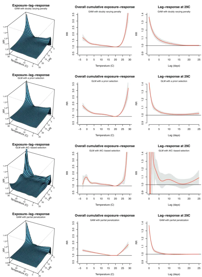
The GAM used 35.45edf to model the dose-lag-response surface, and suggests a strong and short-term association with heat and a more delayed association with cold temperatures, consistently with previous results (Gasparrini et al., 2015). The estimates, reported in the first row of Figure 3, are very similar to those from the original analysis, replicated in the second row. However, it is interesting to note the effect of the double varying penalty in the estimated lag-response at 29◦C, with the curve shrinking toward the null at lags higher than 15. In addition, while the cross-basis specification of the unpe-nalized DLNM was originally defined a priori, an AIC-based selection suggests a very complex and implausible model with 10×9=90df, with estimates illustrated in the third row of Figure 3.

As previously mentioned (Section 3.1), the flexibility of this modelling framework allows a mix of penalized and unpenal-ized functions. As an example, we replaced theps_smoother forf(x) with an unpenalized double-threshold function, that is, linear splines which model a straight relationship below 17◦C and above 21◦C, and a flat region in between. Results are displayed in the last row of Figure 3. This model uses only 10.64edfto define the dose-lag-response surface, although this comes at the price of making strong parametric assumptions for one of the two spaces. The same approach can be used to specify simpler penalized DLMs, by selecting a linear function asf(x).

5.2. Occupational Radon and Lung Cancer Mortality

The second example describes the extension of penalized DLNMs to individual time-to-event data, using a cohort of 3347 miners working in the Colorado Plateau mines, with follow-up at December 31, 1982. Speciﬁcally, the association between an indicator of occurrence of lung cancer death yi,t

for subjectiat aget, and yearly occupational radon exposure

xi,t−, measured in working-level months (WLM), with lags of

2–40 years, was estimated with a Poisson GLM of form: log[E(yi,t)]=α+sx(xi,t−2, . . . , xi,t−40;ηx)

+sz(zi,t−2, . . . , zi,t−40;ηz)+g(t;γ)+δci,t.

(11)

This GLM approximates the Cox proportional hazard model applied in the original analysis (Gasparrini, 2014) by splitting the follow-up time of each individual into 1-year peri-ods, and modelling the baseline risk with a cubic B-spline functiong(t) with 5df. This allows the use of penalized splines implemented within GAMs with survival data. Other terms in the model are a cross-basis functionszto control for the lagged

eﬀect of smoking z, and a linear term for calendar yearc. In the original analysis, the association with radon was modelled with a cross-basis functionsxcomposed of quadratic B-splines

functions with a single internal knot at 59.4 WLM/year and 13.3 years of lag for f(x) andw(), respectively, and bound-ary knots at the respective ranges. The intercept was excluded from the latter, assuming no effect for exposures experienced within the first two years. This model, using a total of 9dfto define the association, was selected by minimizing AIC.

The analysis was replicated with a penalized DLNM using a GAM with a REML estimator, using marginalcr_smoothers with dimension 11 (minus constraints) and 10 for exposure and lag spaces, respectively. The use of the cr _smoother allows placing the knots of the dose-response function f(x) at equally spaced intervals in the log scale, accounting for the highly skewed distribution of radon exposure, and allows excluding the intercept in s() following previous assumptions. In addition to the default penalty on the second derivative, enforced in both spaces, we added a varying ridge penalty of form (7b) tow() withp=1 if >30 and 0 otherwise, thus

assuming no additional risk 30 years after the exposure to radon.

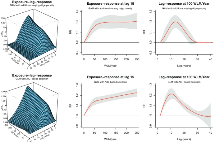
Results are displayed in Figure 4. The penalized DLNM (first row) indicates a peak in lung cancer mortality risk approximately 11 years after the exposure to radon. The non-linear dose-response shows how the risk flattens out above 50 WLM/year. The model used a total of 8.03edfto describe the association. These findings are consistent with the unpe-nalized DLNM fitted with a GLM (second row of Figure 4), which closely approximates the original estimates from the Cox model illustrated by Gasparrini (2014, Figure 2). How-ever, the addition of the ridge penalty in the GAM produces more precise estimates at the end of the lag period, suggest-ing that the risk completely disappears 30 years after the exposure.

6. Discussion

In this contribution, we describe a penalized framework for DLNMs that provides significant developments to this modelling class, through built-in smoothness selection of potentially complex marginal functions and the flexible definition of penalties to accommodate assumptions on the lag structure. This method includes previous smooth-ing approaches for simpler DLMs (Zanobetti et al., 2000; Obermeier et al., 2015) as special cases, and fully extends the penalized approaches to bi-dimensional dose-lag-response surfaces. The DLNM framework unifies methods proposed to investigate lagged associations in different research fields, beyond time series analysis in environmental research. For instance, these include case-control studies in cancer epi-demiology (Thomas, 1988; Hauptmann et al., 2000; Berhane et al., 2008; Richardson, 2009) and survival analysis in

(9)

Tem perature (C) 0 10 20 30 Lag 0 5 10 15 20 25 RR 0.9 1.0 1.1 1.2 1.3 1.4 Exposure−lag−response

GAM with doubly varying penalty

−5 0 5 10 15 20 25 30 0.5 1.0 1.5 2.0 2.5 3.0 3.5

Overall cumulative exposure−response

Temperature (C)

RR

0 5 10 15 20 25 0.9 1 .0 1.1 1 .2 1.3 1.4 Lag−response at 29C Lag (days) RR

GLM with a priori selection

−5 0 5 10 15 20 25 30 0.5 1.0 1.5 2.0 2.5 3.0 3.5

Temperature (C)

RR

0 5 10 15 20 25 0.9 1 .0 1.1 1 .2 1.3 1 .4 Lag−response at 29C Lag (days) RR

GLM with AIC−based selection

−5 0 5 10 15 20 25 30 0.5 1 .0 1.5 2 .0 2.5 3 .0 3.5

Temperature (C)

RR

0 5 10 15 20 25 0.9 1 .0 1.1 1.2 1 .3 1.4 Lag−response at 29C Lag (days) RR

Temper ature (C) 0 10 20 30 Lag 0 5 10 15 20 25 RR 0.9 1.0 1.1 1.2 1.3 1.4 Exposure−lag−response

GAM with partial penalization

−5 0 5 10 15 20 25 30 0.5 1 .0 1.5 2 .0 2.5 3 .0 3.5

Temperature (C)

RR

0 5 10 15 20 25 0.9 1 .0 1.1 1.2 1 .3 1.4 Lag−response at 29C Lag (days) RR

Figure 3. First example: dose-lag-response, overall cumulative dose-response, and lag-response at 29◦C (by column) sum-marizing the association between temperature and all-cause mortality, estimated by a GAM with double varying penalty in the lag space, GLM with a priori selection (as in Gasparrini and Leone (2014)), GLM with AIC-based selection, GAM with partial penalization (by row). London 1993–2006.

(10)

WLM/y ear 0 50 100 150 200 250 Lag (y ears) 5 10 15 20 25 30 35 40 RR 0.95 1.00 1.05 1.10 1.15 1.20 1.25 1.30 Exposure−lag−response

GAM with additional varying ridge penalty

0 50 100 150 200 250 0.9 1.0 1.1 1.2 1.3 Exposure−response at lag 15 WLM/year RR

0 10 20 30 40 0.9 1.0 1.1 1.2 1.3 Lag−response at 100 WLM/Year Lag (years) RR

WLM/y ear 0 50 100 150 200 250 Lag (y ears) 5 10 15 20 25 30 35 40 RR 0.95 1.00 1.05 1.10 1.15 1.20 1.25 1.30 Exposure−lag−response

0 50 100 150 200 250 0.9 1.0 1.1 1.2 1.3 Exposure−response at lag 15 WLM/year RR

0 10 20 30 40 0.9 1.0 1.1 1.2 1.3 Lag−response at 100 WLM/Year Lag (years) RR

Figure 4. Second example: dose-lag-response, dose-response at lag 15, and lag-response at 100 WLM/year (by column) summarizing the association between occupational radon exposure and lung cancer mortality, estimated by a GAM with an additional varying ridge penalty in the lag space and a GLM with AIC-based selection (as in Gasparrini (2014)) (by row). Colorado Plateau Uranium miners cohort, follow-up at December 31, 1982.

pharmaco-epidemiology (Sylvestre and Abrahamowicz, 2009; Abrahamowicz et al., 2012)

This penalized version addresses the problem of choosing the appropriate degree of complexity of the DLNM. This is a critical limitation of traditional unpenalized DLNMs, for which current selection methods are not effective (as demon-strated with the first example in Section 5.1), and produce less efficient estimators (as illustrated in the simulation study in Section 4). This penalized extension is based on well-grounded theoretical results and estimation methods, recently discussed (Wood, 2006a, 2008, 2011), it can be performed with stable and efficient routines implemented in freely available software (Wood, 2006a), and it shows improved inferential properties if compared to the standard unpenalized version.

The results confirm the good inferential properties of REML and UBRE-AIC estimators, with the former appearing slightly superior (Wood, 2011), and the similar performance of alternative types of smoothers (Wood, 2006a). The latter can be selected due to convenient characteristics, such as the possibility of including varying difference penalties with theps smoother (see Section 5.1) or the flexibility in the knots place-ment and exclusion of intercept with the cr _{smoother (see} Section 5.2). In particular, the inclusion of additional penal-ties on the lag dimension provides a way to accommodate realistic assumptions on the underlying shape. These

addi-tional penalties can be selected based on prior knowledge, and do not represent strong constraints on the lag-response shape, as their inﬂuence can be calibrated through the estimate of smoothing parameters. As previously suggested (Muggeo, 2008; Obermeier et al., 2015) and shown in the second scenario of the simulation study, additional penalties can improve the model ﬁt and make the model less sensitive to the choice of the lag period.

Some limitations must be acknowledged. The issue of penal-izing complex bi-dimensional functions has been investigated in a limited set of simulated scenarios and two real-data exam-ples. Also, simulations show some issue with nonconvergence in the simplest scenario, where the selectededftend to be close the null space of the cross-basis function, although this prob-lem does not seem to critically affect inference. The penalized approach substantially improves the coverage properties of the confidence intervals, even though in some scenarios and for some models the empirical coverage falls short of the nom-inal value. In addition, the method presented here shares a known limitation of GAMs, which tend to select simpler (i.e., smoother) models when the statistical power decreases. Finally, smoothing methods for dose-lag-response relation-ships are difficult to validate, as the lag dimension is not directly observable in the data, thus preventing the use of standard techniques such as residual analysis. These issues

(11)

will be hopefully addressed in future research.

Penalized DLNMs can be further extended to varying-coeﬃcients models, describing dose-lag-response relationships that change in time or along the space of other predictors, as previously described for simpler penalized DLMs (Rushworth et al., 2013) or unpenalized DLNMs (Gasparrini et al., 2015). In addition, the DLNM class has interesting links with penal-ized functional regression, where a functional outcome (say the shape of the dose-response) is allowed to vary depending on a functional predictor (say the lag dimension) (McLean et al., 2014; Scheipl et al., 2015), providing the possibility of further extensions through this established modelling frame-work.

Lagged associations occur almost universally in biomedical research, and well beyond. Penalized DLNMs offer a flexi-ble modelling class to describe these phenomena, avoiding biases due to incorrect assumptions about the lag structure, sometimes made when using simpler approaches, and poten-tially extending the knowledge of the association under study. The recent extension of DLNMs beyond time series data (Gasparrini, 2014) unifies and extends methods proposed in different study designs and paves the way for original and promising applications of this modelling framework.

7. Supplementary Materials

Web Appendices, Web Figures, and R code are available at theBiometricswebsite on Wiley OnlineLibrary. In addition to Web Appendices A–B, referenced in Section 4, Web Appendix C brieﬂy describes the software implementation in theR pack-agedlnm. TheRcode fully reproduces the simulation studies and the two examples, with an updated version available from GitHub and the personal website of the ﬁrst author (see Web Appendix C).

Acknowledgements

This work and Dr Gasparrini were supported by a grant awarded by the Medical Research Council-UK (Grant ID:MR/M022625/1), and by a LSHTM Fellowship awarded using Institutional Strategic Support Fund by the Wellcome Trust and the London School of Hygiene & Tropical Medicine (Grant ID: 105609/Z/14/Z). Dr Scheipl was supported by the German Research Foundation through the Emmy Noether Programme, grant GR 3793/1-1 awarded to Dr Sonja Greven.

Conflict of Interest

None.

References

Abrahamowicz, M., Beauchamp, M. E., and Sylvestre, M. P. (2012). Comparison of alternative models for linking drug exposure with adverse eﬀects.Statistics in Medicine31, 1014–1030. Almon, S. (1965). The distributed lag between capital

appropria-tions and expenditures.Econometrica33, 178–196. Armstrong, B. (2006). Models for the relationship between ambient

temperature and daily mortality.Epidemiology17, 624–631. Berhane, K., Hauptmann, M., and Langholz, B. (2008). Using tensor product splines in modeling exposure-time-response

relationships: Application to the Colorado Plateau Uranium Miners cohort.Statistics in Medicine27, 5484–5496. Currie, I. D., Durban, M., and Eilers, P. H. C. (2004). Smoothing

and forecasting mortality rates.Statistical Modelling4, 279–

298.

Eilers, P. H. C., Currie, I. D., and Durban, M. (2006). Fast and compact smoothing on large multidimensional grids.

Com-putational Statistics and Data Analysis50, 61–76.

Eilers, P. H. C. and Marx, B. D. (1996). Flexible smoothing with B-splines and penalties.Statistical Science11, 89–101. Gasparrini, A. (2014). Modeling exposure-lag-response

associa-tions with distributed lag non-linear models. Statistics in

Medicine33, 881–899.

Gasparrini, A., Armstrong, B., and Kenward, M. G. (2010). Dis-tributed lag non-linear models. Statistics in Medicine29, 2224–2234.

Gasparrini, A., Guo, Y., Hashizume, M., Kinney, P. L., Petkova, E. P., Lavigne, E., et al. (2015). Temporal variation in heat-mortality associations: A multi-country study.

Environ-mental Health Perspectives123, 1200–1207.

Gasparrini, A., Guo, Y., Hashizume, M., Lavigne, E., Zanobetti, A., Schwartz, J., et al. (2015). Mortality risk attributable to high and low ambient temperature: A multicountry observational study.The Lancet386, 369–375.

Gasparrini, A. and Leone, M. (2014). Attributable risk from dis-tributed lag models. BMC Medical Research Methodology

14, 55.

Green, P. J. and Silverman, B. W. (1994).Nonparametric Regres-sion and Generalized Linear Models: A Roughness Penalty Approach. Monographs on statics and applied probability 58. London: Chapman & Hall.

Hastie, T. and Tibshirani, R. (1990).Generalized Additive Models, 2nd edition, London: Chapman & Hall/CRC,.

Hauptmann, M., Wellmann, J., Lubin, J. H., Rosenberg, P. S., and Kreienbrock, L. (2000). Analysis of exposure-time-response relationships using a spline weight function.Biometrics56, 1105–1108.

Marra, G. and Wood, S. N. (2012). Coverage properties of conﬁ-dence intervals for generalized additive model components.

Scandinavian Journal of Statistics39, 53–74.

McLean, M. W., Hooker, G., Staicu, A.-M., Scheipl, F., and Rup-pert, D. (2014). Functional generalized additive models.

Journal of Computational and Graphical Statistics23, 249–

269.

Muggeo, V. M. (2008). Modeling temperature eﬀects on mortality: Multiple segmented relationships with common break points.

Biostatistics9, 613–620.

Obermeier, V., Scheipl, F., Heumann, C., Wassermann, J., and Kuhchenhoﬀ, H. (2015). Flexible distributed lags for mod-elling earthquake data. Journal of the Royal Statistical

Society: Series C64, 395–412.

Richardson, D. B. (2009). Latency models for analyses of protracted exposures.Epidemiology20, 395–399.

Rushworth, A. M., Bowman, A. W., Brewer, M. J., and Langan, S. J. (2013). Distributed lag models for hydrological data.

Biometrics69, 537–544.

Samet, J. M., Zeger, S. L., Dominici, F., Dockery, D., and Schwartz, J. (2000). The National Morbidity, Mortality, and Air Pollution Study (NMMAPS). Part 1. Methods and method-ological issues. Technical report, Health Eﬀects Institute. Scheipl, F., Staicu, A.-M., and Greven, S. (2015). Functional

addi-tive mixed models.Journal of Computational and Graphical

Statistics24, 477–501.

Schwartz, J. (2000). The distributed lag between air pollution and daily deaths.Epidemiology11, 320–326.

(12)

Sylvestre, M. P. and Abrahamowicz, M. (2009). Flexible modeling of the cumulative eﬀects of time-dependent exposures on the hazard.Statistics in Medicine28, 3437–3453.

Thomas, D. C. (1988). Models for exposure-time-response rela-tionships with applications to cancer epidemiology.Annual

Review of Public Health9, 451–482.

Welty, L. J., Peng, R. D., Zeger, S. L., and Dominici, F. (2009). Bayesian distributed lag models: Estimating eﬀects of par-ticulate matter air pollution on daily mortality.Biometrics

65, 282–291.

Wood, S. N. (2006a).Generalized Additive Models: An Introduction with R. Boca Raton, FL: Chapman & Hall/CRC.

Wood, S. N. (2006b). Low-rank scale-invariant tensor product smooths for generalized additive mixed models.Biometrics

62, 1025–1036.

Wood, S. N. (2008). Fast stable direct ﬁtting and smoothness selec-tion for generalized additive models. Journal of the Royal

Statistical Society, Series B70, 495–518.

Wood, S. N. (2011). Fast stable restricted maximum likelihood and marginal likelihood estimation of semi-parametric general-ized linear models.Journal of the Royal Statistical Society,

Series B73, 3–36.

Zanobetti, A., Wand, M. P., Schwartz, J., and Ryan, L. M. (2000). Generalized additive distributed lag models: Quantifying mortality displacement.Biostatistics1, 279–292.

Received September 2015. Revised October2016. Accepted November2016.