Fast high dimensional approximation via random embeddings

(1)

Copyright by

Christopher Garrett Kennedy 2018

(2)

The Dissertation Committee for Christopher Garrett Kennedy certifies that this is the approved version of the following dissertation:

Fast High Dimensional Approximation via Random

Embeddings

Committee:

Rachel Ward, Supervisor Fran¸cois Baccelli

Andrew Blumberg Eric Price

(3)

Fast High Dimensional Approximation via Random

Embeddings

by

Christopher

Garrett

Kennedy

DISSERTATION

Presented to the Faculty of the Graduate School of The University of Texas at Austin

in Partial Fulfillment of the Requirements

for the Degree of

DOCTOR OF PHILOSOPHY

THE UNIVERSITY OF TEXAS AT AUSTIN December 2018

(4)

Acknowledgments

First and foremost, I thank my advisor Rachel Ward for her continu-ous support throughout my graduate career. I also thank my committee for agreeing to supervise this thesis, and for the time and feedback they dedicated to it.

I thank my parents Tom and Diana, for their unending guidance. Thank you to all the friends who have made my days better in every way.

Many UT staff have been invaluable and timely throughout this process, I would especially like to thank Elisa Armendariz, Dan Knopf, Sandra Catlett, and Tim Perutz.

(5)

Fast High Dimensional Approximation via Random

Embeddings

Publication No.

Christopher Garrett Kennedy, Ph.D. The University of Texas at Austin, 2018

Supervisor: Rachel Ward

In the big data era, dimension reduction techniques have been a key tool in making high dimensional geometric problems tractable. This thesis focuses on two such problems - hashing and parameter estimation. We study locality sensitive hashing(LSH), which is a framework for randomized hashing that efficiently solves an approximate version of nearest neighbor search. We propose an efficient and provably optimal hash function for LSH that builds on a simple existing hash function called cross-polytope LSH. In the context of parameter estimation, we focus on regression, for which the well-known LASSO requires precise knowledge of the unknown noise variance. We provide an estimator for this noise variance when the signal is sparse that is consistent and faster than a single iteration of LASSO. Finally, we discuss notions of distance between probability distributions for the purposes of quantization and propose a distance metric called the R´enyi divergence, that achieves both large and small scale bounds.

(6)

List of Tables

3.1 Optimal window sizes as a function of α, kβk2. . . 33

3.2 σ and λ values for real data sets. . . 40 4.1 Various LSH Families and corresponding Hash Functions. . . 58

(9)

List of Figures

3.1 LASSO estimators with window size based on inflection point. 31

3.2 LASSO estimators with optimal window size. . . 32

3.3 LASSO estimators in the high dimensional regime. . . 34

3.4 LASSO estimators with orthogonal design matrix. . . 36

3.5 LASSO estimators with dense signal. . . 38

3.6 MSE for 10-fold CV LASSO using data from [57], with the λ value given by the estimator from Algorithm 2 marked in magenta. 41 3.7 MSE for 10-fold CV LASSO using data from [5]. . . 42

3.8 MSE for 10-fold CV LASSO using data from [27]. . . 43

4.1 LSH collision probabilities, d= 128, d0 = 128 . . . 72 4.2 LSH collision probabilities, d= 128, d0 = 64 . . . 72 4.3 LSH collision probabilities, d= 128, d0 = 32 . . . 72 4.4 LSH collision probabilities, d= 256, d0 = 256 . . . 73 4.5 LSH collision probabilities, d= 256, d0 = 128 . . . 73 4.6 LSH collision probabilities, d= 256, d0 = 64 . . . 73

4.7 LSH collision probabilities by dimension, R = 0.4 . . . 74

4.8 LSH collision probabilities by dimension, R = 0.7 . . . 74

4.9 LSH collision probabilities by dimension, R = 1 . . . 75

(10)

Chapter 1 Introduction

Often for problems involving large amounts of data in very high dimen-sion, computing even simple properties of the data set, for example pairwise distances, can be prohibitively expensive to compute and store. To illustrate this, consider a collection of 1 billion vectors of length 10000 (for example, a database of images). Computing the distance between two vectors in MAT-LAB on my laptop takes roughly 3∗10−5 seconds, which seems fast, but to even find the nearest neighbor (by computing all pairwise distances with a point) would take 5 and a half hours. There are two fundamental approaches to dealing with these kinds of bottlenecks:

• Develop a better algorithm to the problem or a relaxation of the problem that doesn’t require brute force computation.

• Reduce the dimensionality of the data to improve storage and computa-tion time.

In this work we explore applications of both these techniques using modern tools from random matrix theory. The main problems we are solving, detailed below, are nearest neighbor search and regression. In both cases we assume

(11)

the dimension of the data is very high and, in the case of nearest neighbor search, there are a lot of data points.

Common techniques for reducing the dimensionality of data include principal components analysis (PCA) and all of its’ variants, as well as non-linear methods such as self-organizing maps, autoencoders, kernel-PCA, etc. However, these methods suffer from inefficiency on high-dimensional data, ei-ther in the preprocessing or embedding step. In this work, we use subsampled, fast matrices such as the Fast Fourier Transform (FFT). Although this choice of matrix is classical and well-studied, the theory behind its’ use as a tool in dimension reduction is much more recent. We also employ the following principle, from [37], which extends the use of these matrix ensembles:

Reducing the dimension of a finite point set and reducing the dimension of the set of all sparse vectors, while preserving pairwise distances, are “nearly”

equivalent.

“Nearly” has a precise quantitative meaning which we will see later. This principle allows us to use fast dimension reducing matrices like subsampled FFTs in problems like regression, where the underlying structure of some estimator is sparse. In particular, we use the (fast) matrix ensembles used in compressed sensing because they preserve distances on sparse vectors, can also be used as dimension reducing matrices. This allows us to show our methods are both (i-) provably efficient and (ii-) provably work for their corresponding geometric problems.

(12)

1.1 Nearest Neighbor Search

Suppose we are given a set of pointsP ={x1, ..., xn} ⊂ X in a metric

space (X,D). The fundamental task we are trying to solve is to find the nearest neighbor in our dataset.

Definition 1. (Exact Nearest Neighbor) Given a query point p ∈ P, return the pointq ∈P that minimizes

q:= argmin_p₀_∈_RD(p0, p).

The naive algorithm simply computes the pairwise distances D(p0, p)

for everyp0 ∈P and keeps a running index of the minimum. For euclidean

dis-tance inX =_Rd_{, this algorithm runs in time}_O_{(nd) and becomes prohibitively}

expensive when n, d 0. The typical problem that occurs when trying to improve this bound, in other words to achieve sublinear query time, is that the storage requirements scale on the order ofnO(d)_{. This exponential growth}

is suspected to be unavoidable except in problems with additional structure (i.e.if the data lies in a low-dimensional manifold), and is a manifestation of the “curse of dimensionality.”

In order to circumvent this, one needs to relax the problem we are trying to solve. Specifically we replace the exact nearest problem with approximate nearest neighbor search. The meaning of “approximate” can vary, but for our purposes it means the following.

(13)

Definition 2. (Approximate Nearest Neighbor)Givenp∈P andc, R > 0 and suppose that ∃p0 ∈ P s.t. D(p0, p)< R. Return (with high probability)

q ∈P s.t. D(p, q)< cR.

It should be clear that this problem is a relaxation of nearest neighbor search in the case thatc >1, and in general the performance of any algorithm should degrade asc&1. In fact, forc= 1, one can formulate an algorithm for nearest neighbor search by varying R > 0. For now, we fix our metric space X ⊂_Rd _{with the Euclidean metric.}

One way to approach approximate nearest neighbors is to instead do a preprocessing step that involves randomly hashing each point inP, then look-ing for collisions in the hash maps. This requires careful choice of hash map, because for this algorithm to work we need the hash function to be more likely to map close points to the same hash value - so called Locality Sensitive Hashing (LSH). The cost for improved query time is in precomputing the hash values of every point.

From the above discussion, it should be clear that there is a tradeoff between:

(i-) Query time

(ii-) Number of hash computations for each point (iii-) Time to hash individual points.

(14)

Items (i-) and (ii-), as we will see later, can be simultaneously minimized using a parameter called “sensitivity,” which quantifies how well our hash function detects whether points are close. In fact, hash functions have been constructed that achieve the (asymptotically) optimal lower bound in terms of sensitivity, as d → ∞, but they are either hard to implement or have inefficient hash computations.

As suggested in the first section, our approach to develop a more ef-ficient algorithm for LSH is to project our points via some FFT-type matrix M : _Rd_→

Rm where m d, then hash our points in dimension m in such a

way that the sensitivity is preserved. The main advantage is that we replace a typically dense matrix from_Rd→_Rd_{with a fast, structured projection matrix.}

This allows us to do the hashing operation onm-dimensional points, which is significantly faster when m = O(polylogd). Our algorithm is adapted from a previously studied scheme called cross-polytope LSH. It is easy to implement and has properties that a straightforward to analyze using results on high-dimensional Gaussians. This allows us to bootstrap our analysis on previous results in a very straightforward way.

1.2 Regression

We now turn to the problem of regression analysis. In it’s simplest form, the problem is the following.

Definition 3. Given y ∈ _Rn_, _X _∈

Rn×p known and some unknown signal

β ∈ _Rp _{such that} _y ₌ _Xβ ₊_η _where _η _∈

(15)

return βbthat minimizes

b

β := argmin_β₀_∈_Rpkβ−β₀k_r,

for somer.

Obviously if the noise is unknown the above problem is in general in-tractable. We make the simplifying assumption thatη∼N(0, σ2) is Gaussian with small variance. Of course whenn ≤p, r = 2, and there is no noise, the problem can be solved exactly as βb= X†y, where X† := (XTX)−1XT is the

pseudoinverse.

We work in the case wherep n, where least squares is less effective. Note that least squares cannot distinguish between solutions modulo the null space ofX, and can potentially lose a lot of information about the desired β. For the problem to be more tractable, we make the assumption that β ∈ _Rp

is s-sparse. We can think of s as having very small growth compared to the other variables in the problem. Typical methods for solving the regression problem whenpn need an accurate estimation of the variance of the noise. Intuitively, this estimate should tell the algorithm how much it should try to fit the estimate β to the transformed signal y. The LASSO solves a convex optimization problem that balances fitting the signal and a regularization term (typically some norm of the estimatedβ) to prevent overfitting. In particular, we minimize

b

β = argmin_βkXβ−yk2

(16)

whereλ is tuned according to the variance of the noise. If the exact noise level is known, there are a large class of results called oracle inequalities that provide bounds onkβb−βk_r (whereβbis the solution to the LASSO objective)

for various values of r≥1.

Recall that β is s-sparse (with unknown level of sparsity), so ideally we would use the `0 norm in (1.1) to promote sparsity. However, even if the

level of sparsity is known this penalization requires checking all O(ns₎

possi-ble supports of β, which is intractable for even moderately sized s. On the other hand, we can replace the `1 norm with kβk22, which actually leads to a

closed form solution. This is called ridge regression or Tikhonov regulariza-tion. However, as we will see later, the solution to this penalization also has undesirable properties. There is a variant of ridge regression that uses a linear combination of the `2 and `1 penalty terms, called the elastic net [73].

Our approach deviates from the LASSO penalization, and seeks to ex-ploit the sparse structure of β using short, fast matrices typically used for dimension reduction. We first compute XTy (where X is the design matrix from above) and then take averages of the small entries of the resulting vec-tor. The hope is that, provided the matrixXT _{behaves “well” with respect to}

the sparse vector β, the small entries capture information about the variance (remember the above assumption that the noise variance is small compared to the signal). The bulk computational step is a simple matrix/vector multiplica-tion. This is beneficial both because it is extremely simple to implement and also because this operation is highly optimized in most languages and easily

(17)

parallelizable.

1.3 Robust Quantization

For the above problems, we are attempting to recover simple geomet-ric information based on incoming data. In the case of LASSO, we want to recover the variance of the noise in the received vector, and in LSH we want to efficiently recover nearest neighbors from a given query point. Typically we want to evaluate the performance of the algorithm - in the case of LASSO, the variance and corresponding λ parameter, and for LSH the randomized hash maps. In this section we generalize this framework to evaluate the performance of a pre-trained algorithm on some incoming data set.

The algorithmic framework we use that is very natural in the geomet-ric setting is quantization. Formally, quantization will partition the space into various regions and hash it according to this partition, mapping the contin-uous space to a discrete set of partition elements. We make the additional simplifying assumption that our partition scheme is a Voronoi partition, i.e. that each partition element is the set of points closest to a given point accord-ing to some metric. Thus, a quantization scheme corresponds to an indexed set of pairs Q = {(Pi, wi)} ⊂ Rd×Rd, where each wi is a point in Rd and

Pi ={x∈Rd :D(x, wi)≤D(x, wj)∀j}.

Fix our distance to be the Euclidean metric, and assume our quantiza-tion scheme is well adapted to some distribuquantiza-tion _P1. To quantify this, define

(18)

the quantization error E_P₁,Q :=

Z

Rd

`(x,argmin_w_ikx−wik2)dP1(x),

for some loss function`. This is enough to guarantee a hash function based on a voronoi partition (as is common in LSH) is well-adapted to a distribution_P1.

In addition to this global geometric property, we would like to also capture localbounds on small probability events.

Suppose we receive samplesqi ∼P2 from a new distribution P2. There

are two fundamental questions we investigate:

• What notion of closeness between _P1 and P2 will make the quantization

schemeQhave low error for both distributions (also, can we extend these to finite sample bounds).

• What notion of closeness will ensure that small probability events ac-cording to _P1 will also have small probability in P2, i.e. scale invariant

bounds.

Note that the second item above allows for analysis of nearest neighbors in the context of a quantization scheme.

There are various divergence and transportation based distance metrics between probability distributions. Among the most popular are the Wasser-stein distance and the Kullback-Leibner(KL) divergence. We will see in sec-tion 5, both of these nosec-tions are insufficient for satisfying both condisec-tions

(19)

listed above. Instead, we use a generalized KL divergence known as the R´enyi divergence, Rα(P1kP2) := 1 α−1ln EP2 d_P1 d_P2 α .

It can be shown that this approaches the R´enyi divergence in the limit α↓1. This notion of distance turns out to be appropriate for all of the purposes outlined above, and classifies proximity between the distributions _P1 and P2

in both global and local properties.

1.4 Main Results

1.4.1 Fast Cross-Polytope LSH

There are many choices of hash functions in LSH that have various advantages/disadvantages many of which we will mention later. One that we will focus on because it has optimal asymptotic sensitivity and a very simple formulation is cross-polytope LSH: h(x) = argmin u={±ei} Gx kGxk2 −u 2 . (1.2)

Here, G ∈ _Rd×d _{is a Gaussian matrix with i.i.d.} _N_(0,_{1) entries, so that} _x

is rotated uniformly at random, then rounded to the nearest ± unit vector ei. This function has the obvious disadvantage that it takes time O(d2) to

compute. We replace the matrix G with a fast alternative G0 : _Rd → _Rd0

which supports matrix/vector multiplication in time O(dlnd). Our new hash function becomes h(x) = argmin u={±ei} G0_x kG0_x_k 2 −u 2 . (1.3)

(20)

The choice ofd0can vary and can be tuned for desired sensitivity/runtime, but for now we choose d = d0. Our main result about this version of cross-polytope LSH is the following.

Theorem 4. Consider the hash family H defined by (1.3). Then, H has the optimal rate of convergence in sensitivity as d → ∞ and supports time

O(dlnd) hash computation.

Using a construction from [33], we can replace our subsampled FFT with a matrix that has only O(polylogd) random bits. With this and a similar construction, we can extend our result.

Theorem 5. There is a hash familyHb that has the optimal rate of convergence

in sensitivity as d → ∞, supports time O(dlnd) hash computation, and only requires O(polylogd) bits of randomness.

One big omission thus far is the precise meaning of sensitivity, and also the optimal rate of convergence. These definitions, as well as proofs of theorems 4 and 5 will be given in section 4. In section 4.6, we illustrate the collision probability of our scheme compared to regular cross-polytope LSH for various distances. We also highlight the collision probabilities by dimension, versus the optimal rate mentioned above.

1.4.2 Regression

Our estimator for noise variance has a very simple formula for the case where p = n and X ∈ _Rp×p _{is orthogonal. Note that for the purposes of}

(21)

estimating the noise variance, X is the identity w.l.o.g., so that we receive a noisy signaly=β+η. We state the orthogonal estimator here because of it’s simplicity:

1: Compute the window estimators Sj = _L1 P_i∈Ωj|yi|

2_{, j} _{∈ {}_1,_{2, . . . , p/L}_}_. 2: Let σb2 = (1 + 1 log(p)) 2L p Pp/(2L)

j=1 S(j), where {S(j)}j is a non-decreasing

ar-rangement of {Sj}j.

The above estimator is extremely efficient to compute, in fact the most expensive step is computing the window estimators (assuming the number of Ωj is relatively small, so that sorting is cheap). Additionally, it works well in

typical regimes.

Theorem 6. Supposey=Xβ+ηwhereX ∈_Rp×p _{is orthogonal,}_η

j ∼N(0, σ2)

are independent and β is s-sparse. For window size

L= O(polylog(p)) and sufficiently small s, the above variance estimator sat-isfies |σb2−σ2| ≤ 6σ2 logp, with probability 1− 2 p.

We can extend our estimator to the case where p > n. In this case, the estimator is nearly identical, but first we preprocess the vectory via mul-tiplication by XT _where _X _{is the design matrix, and then apply the above}

method. As we will see in section 3, assuming X is sufficiently “nice” we can use this preprocessing step to exploit the sparsity of β. This is additionally a use of the principle mentioned earlier this section, that matrices typically

(22)

used for dimension reduction also preserve distance of sparse vectors. For this estimator, we have the following result.

Theorem 7. Suppose y = Xβ + η where X ∈ _Rn×p _{is sufficiently}

well-behaved, ηj ∼ N(0, σ2) are independent and β is s-sparse. For window size

L = O(polylog(p)), n ≥L and sufficiently small s, then the generalized vari-ance estimator satisfies

|_bσ2−σ2| ≤ Cδ,β,p

log(p)(σ

2

+ 1).

We hide the constantCδ,β,p in the above theorem for simplicity, but it

approaches 0 at a rate of O(1/polylog(p)) in typical regimes.

The full version of the above estimator and theorem will be given in sec-tion 3. The proofs rely on combining properties of the matrixXT _{when applied}

to the sparse vector β, and standard concentration results. We also provide an empirical comparison to other standard variance estimators in section 3.4 as well as results on well known genomics data sets.

1.4.3 Quantization

Using the R´enyi divergence mentioned above, we can formulate our first result, a scale invariant bound between two probability distribution _P1 and P2. Note that for the R´enyi divergence to exist, P1 and P2 must be mutually

absolutely continuous, but this is a necessary property for such a bound. Our first result in the follow.

(23)

Proposition 8. Suppose _P1 and P2 are probability distributions that are

mu-tually absolutely continuous. Then, for all events E,

P2(E)(α−1)/αexp[−(α−1)Rα(P2kP1)]≤P1(E)

≤_P2(E)α/(α−1)exp[(α−1)Rα(P1kP2)].

This result also implies a multiplicative bound between the quantization error of _P2, EP2,Q and the quantization error of P1, EP1,Q according to some scheme _P2 (we drop the subscript Q in our notation and assume this scheme

is fixed):

exp[−(α−1)Rα(P2kP1)]EP2 ≤EP1 ≤exp[(α−1)Rα(P1kP2)]EP2. Making a further assumption that the distributions are supported in a ball of radiusR >0, we can use concentration inequalities to get finite sample bounds on the quantization error of an incoming set of pointqi ∼P2.

Proposition 9. Suppose that _P1 and P2 are mutually absolutely continuous,

such that

Rα(P1kP2), Rα(P2kP1)≤δ, for some α >1, δ >0. Suppose also that we have

some fixed quantization scheme Q with error E_P₁ < on distribution _P1 and

>0 small, and we receive {qi}Ni=1 ∼P2. Then, P2(|dE_P₂ −E_P₁| ≥t+C_R,δ,,α)≤2 exp ₋ 2N t2 R2 . (1.4)

The constantCR,δ,,α →0 asδ→0. Roughly, the proposition says that

(24)

error as the number of points goes to infinity, and the R´enyi divergence between the distributions goes to 0.

We note that these results can be leveraged to achieve bounds on more precise events, such as the probability that the k nearest neighbors land in the same Voronoi cell (i.e. partition element of the quantization scheme) for some k, but the parameters become unmanageable. These considerations are beyond the scope of this work.

(25)

Chapter 2 Background

2.1 Dimension Reduction Techniques

A key technique throughout this work and a common theme across all high-dimensional data analysis is to first reduce the dimension of the data while preserving some important property of the data set (pairwise distances, ordering, etc). Typically, given a set of points P ={x1, ..., xn} ⊂Rd, one finds

a linear mapA:_Rd_→

Rm wherem=O(polylog(n)) that is sufficiently “nice”

for practical purposes, for example

(1−δ)kxi−xik22 ≤ kA(xi−xj)k22 ≤(1 +δ)kxi −xjk22, ∀i6=j. (2.1)

We call a map satisfying the above property aJohnson-Lindenstrauss (JL) Transform. This property is especially important when the problem we are solving involves some geometrical property of the data, since pairwise distances are approximately preserved. The most natural map we can choose is to take Ato be a uniformly random projection onto ann-dimensional subspace of_Rd. A typical way to do this is to generate a matrix G ∈_Rn×d _{with i.i.d.} N_(0,₁₎

entries and then compute A = U VT_{, where} G ₌ _U_ΣVT _{is the SVD of} G_{. In}

(26)

Theorem 10. [32] For any0< δ <1/2, any point setP ⊂_Rd _{of size}_{n, and}

m=O(log(n)δ−2₎ _{there is a map} _A_:

Rd→Rm such that (2.1) holds.

Moreover, there is a construction where the map f is linear and the choice m = O(log(n)δ−2) is optimal over all linear maps ( [4], [38]). Much work has gone into finding fast JL-transforms that get as close as possible to this bound. Following a strong line of work ( [1], [2], [37], among others), a fast JLT can be constructed as follows:

A =HSDb.

Here,Db :Rd →Rdis diagonal with i.i.d. Rademacher entries on the diagonal,

andHS ∈Rm×dis a partial Hadamard matrix restricted to a uniformly random

subset of|S|=mrows. Many versions of this transform occur in the literature, sometimes replacing the Hadamard matrix with a different orthogonal matrix (fast fourier tranform, e.g.), replacing the row subset with a sparse Gaussian, and without or without the diagonal Rademacher matrix.

2.1.1 Restricted Isometry Property/Connections

We now develop a distinct but related notion, the Restricted Isometry Property. As the name suggests, this property ensures our matrix is a near isometry on a restricted subset of_Rd_{, notably all sparse vectors up to a certain}

order.

(27)

Propertyof (integer) order s0 >0 and level δ >0 if

(1−δ)kxk2 ≤ kAxk22 ≤(1 +δ)kxk 2

2 for all s0-sparse x∈Rd.

It should be clear that in general, we can’t say that a RIP matrix will be a near isometry on any given point set (this would imply it is an isometry on the whole space). However, if instead our matrix comes from a distribution that satisfies RIP of some order/level with high probability, then it is a probabilistic JL-transform. Specifically, we say a matrix A ∈ _Rm×d

sampled from some distribution is a probabilistic JL-transform if

P(1−δ)kxk22 ≤ kAxk 2 2 ≤(1 +δ)kxk 2 2) ≥1−2 exp(−c0δ2m), (2.2)

for fixedx∈_Rn _{and some constants}_c

0,δ >0 (c0 may have mild dependencies

on the other parameters). Note that this statement can easily be translated to a concentration inequality over a set of points via union bounds. We now have the following deep result from [11].

Theorem 12. (Theorem 5.2 from [11]) Fix m, d, δ > 0. Suppose that A ∈ Rm×d comes from a distribution satisfying 2.2 for some c0 > 0. Then, there

are absolute constants c1, c2 such that with probability 1−2 exp(−c2δ2m) the

matrix A satisfies RIP of order s0 ≤c1δ2m/ln(d/s0) and level δ >0.

Thus, the probabilistic JL condition satisfies RIP with high probability. There is also a partial converse:

Theorem 13. (Theorem 1.3 from [37]) Fix η, δ > 0 and some finite set E ⊂ _Rd _{of cardinality} _|_E_| ₌ _{p. Suppose that} _A _{satisfies RIP of order} _s

(28)

40 ln(4p/η) and level δ. Let b ∈ {−1,1}d _{be an i.i.d. Rademacher sequence.}

Then, with probability ≥1−η, (1−δ/4)kxk2

2 ≤ kADbxk22 ≤(1 +δ/4)kxk 2 2

for all x∈E.

This theorem should give justification to the construction in the pre-vious section, since a Hadamard matrix restricted to a uniformly random row subset satisfies RIP with high probability, thus multiplying it by a diagonal matrix with i.i.d. signs on the diagonal makes it also act as a JL transform on some fixed subset with high probability. These two theorems give a precise quantitative version of the principle from the introduction, that reducing the dimension of a finite point set and the set of all sparse vectors are “nearly” equivalent.

2.2 Regression and the LASSO

Consider the following setting: suppose β ∈ _Rp _is _{s-sparse, and that}

we are given a noisy, transformed version of this signal, y=Xβ+η.

Here η ∈ _Rn _{has i.i.d. Gaussian entries} _η

j ∼ N(0, σ2) and X ∈ Rn×p is a

known design matrix. The regression problem is to find an estimator βbthat

minimizes the mean squared error (MSE), MSE(β) :=b E b β h kXβb−yk2₂ i . (2.3)

(29)

A key observation is that the above error can be decomposed into bias and variance terms,

MSE(β) = Var(Xb β) + Bias(Xb β) +b σ2. (2.4)

Minimizing both terms simultaneously is a classical problem in statistics - we don’t want to overfit by minimizing bias and get a high variance estimator, or underfit by minimizing variance resulting in higher bias.

Suppose, in the above setting, thatp≤n, so that our matrixX ∈_Rn×p

is potentially overdetermined. In this case we can directly minimize the bias,

b

2 =X

†

y,

whereX† = (XT_X)−1_X _{is the pseudoinverse of}_{X. The obvious drawback of}

the above method is that the variance of this estimator can be large, and also if p > n, it is not uniquely defined. Instead, it is common to add a regularization term to prevent overfitting:

b

β = argmin_βkXβ−yk2₂+λf(β). (2.5) The parameter λ >0 is tuned to the amount of counterbalance we want, and the function f can vary based on application. In general, this problem no longer has a closed form solution, and for some choices of f it can be highly non-convex. We focus on the case wheref(β) = kβk1 so that the above

objec-tive is convex, and the minimization is called LASSO (least absolute shrinkage and selection operator). In the vein of many ideas from Compressed Sensing,

(30)

one can think of the choice of`1 norm as a proxy for the `0 norm to promote

sparsity (however, choosing f(β) =kβk0 makes the problem intractable).

In-tuitively, the LASSO is selecting the “important” entries ofβthat will improve generalization error.

Remark 14. (Ridge Regression) If instead we take f(β) =kβk2

2, the resulting

minimization is called ridge regression or Tikhonov regularization. Instead of promoting sparsity, the euclidean norm imposes a large penalty for large entries, which shrinks the entries of β to prevent overfitting. However, unlike the LASSO this method doesn’t tell us which entries are important (useful in the case where pn), which makes the resulting estimator less interpretable.

(31)

Chapter 3 Variance Estimation for the LASSO

This section is based on work that appears in the preprint [35]. Recall that LASSO attempts to recover a noisy, transformed signal Y = Xβ +η where η ∈ _Rn _{has i.i.d. Gaussian entries} _η

j ∼ N(0, σ2), X ∈ Rn×p is known,

and β ∈_Rp _is _{s-sparse, using the following minimization,} b

2+λkβk1.

The standard analysis of the LASSO is conditioned on the event {λ : λ/4 ≥ kXT_η_k∞_/n_} _{(see [14]). In particular, for the case that} _η _{is Gaussian}

with variance σ2 _and _X _∈

Rn×n is orthogonal, with high probability we have kXT_k∞_/n _{= Θ(σ}2_{log(n)/n). Thus, with the choice} _λ _{= 4σ}2_{log(n)/n, the}

LASSO will provably produce a good estimate β.

However, in applications, the variance σ, and hence a proper choice of λ, is not known a priori. We consider the case where σ is not known in advance, and needs to be estimated from the signal y. It should be clear from the above observations that precision in estimating the parameter σ improves recovery of the true signal.

(32)

3.1 Standard Methods

A good review of variance estimators for LASSO is given in [53], where variance estimation using cross-validated LASSO is highlighted as particu-larly strong in many sparsity regimes. This method typically uses 5 or 10-fold cross-validation to train the hyperparameters in LASSO and analysis relies on the restricted eigenvalue condition on the design matrix. The above work was later complemented by a theoretical analysis of a slightly modified vari-ant of cross-validated LASSO in [18] (see also [23] [29], e.g.). The method of moments (see [21]) is a reasonable alternative to cross-validated LASSO. It relies on the assumption that the design matrix is Gaussian and exploits statistical properties to formulate an estimator. It is consistent with a good rate of convergence [21], but the design matrix has to be Gaussian which is restrictive. We should also mention a variant of the LASSO - the square-root LASSO (see [13]) - whose penalty level doesn’t depend on the variance of the noise. However, the resulting estimator is formulated as a conic programming problem which can be inefficient in practice and is beyond the scope of this work.

3.2 Greedy Variance Estimation – The Orthonormal

Case

For the moment we focus on the case whereX ∈_Rp×p_{is an orthonormal}

matrix (p=n) and the problem reduces to recovering the noisy signaly=β+η (by rotational invariance of the Gaussian). In this regime, the LASSO has the

(33)

closed form solution

b

βi = sign(yi)(|yi| −λ)+,

whereβb_i =βb_i(λ) implicitly depends onλ. A standard approach is to minimize

the cross-validation error:

min

λ ky− b

β(λ)k2,

which has nice practical and theoretical properties (see [36] e.g.). Moreover, given the optimalλone can infer a good estimate of the variance askβb−yk₂/p.

However, this approach still requires one to compute the LASSO minimizer over a range ofλ values, whereas one would like to perform a single computa-tion to estimate the variance (and thus optimal λ). We formulate a method to estimate the variance which only needs a single pass over the input y. Algorithm 1 Greedy Variance Estimator – Orthonormal Design Matrix

1: Compute the window estimators Sj = _L1 P i∈Ωj|yi| 2_{, j} _{∈ {}_1,_{2, . . . , p/L}_}_. 2: Let σb2 = (1 + 1 log(p)) 2L p Pp/(2L)

j=1 S(j), where {S(j)}j is a non-decreasing

ar-rangement of {Sj}j.

The basic idea behind the above algorithm is that we want to capture a noise estimator that avoids the entries of y affected by signal (hence in the second step we take the average of the smaller 50% of the window estimates). We multiply the resulting estimator by 1 +_log(1_p₎ to correct the downward bias that results from averaging only over the smallest windows.

Remark 15. (Total variation denoising) Suppose we receive image-type data and instead of taking the LASSO minimizer we want to instead want to

(34)

regu-larize by the total variation seminorm: b β =argmin β kβ−yk 2 2+ 2λTV(β), (3.1) where TV(β) :=P

nkβn−βn−1k. The typical assumption in this model is that

the discrete derivative of true signal is sparse, which is promoted by the above objective. In this case, we can apply our estimator to the discrete derivative (which as observed is essentially a sparse signal plus noise) to get a reasonable estimate of the variance of the noise in this setting. This approach originally appeared in [56] and statistical guarantees on the resulting estimator βb have

been developed in [44], [47], [67], culminating most recently in [30]. These papers give a framework that allows one to generalize the estimator (3.1) to when the signal is 2-D image data. We note that our estimators can also be easily adapted to 2-D image data by replacing window estimates with box estimates.

We have the following result which guarantees accuracy of the estimatorσb2.

Theorem 16. Suppose y = Xβ+η where X ∈ _Rp×p _{is orthonormal,} _η j ∼

N(0, σ2₎ _{are independent, and} _β _is _s-sparse. _{Consider window size} _L _≥

log3(p), and suppose that s ≤ p

2L. Then the Greedy Variance Estimator

pro-duced by Algorithm 1 satisfies

|σb2−σ2| ≤ 6 logpσ 2_, with probability 1− 2 p.

(35)

3.3 Greedy Variance Estimation – RIP Design Matrix

We now turn to the more general case where the design matrix X ∈ Rn×p is possibly underdeterminedn ≤p,but satisfies the Restricted Isometry

Property with the appropriate constants (indeed this is a more general case, as an orthonormal matrix satisfies the RIP with constant δ = 0). We define the regularized design matrix asZ := [ZΩ1, ..., ZΩp/L] where each ZΩi ∈R

n×L_,

ZΩi :=UiIn×LVi such that (3.2)

XΩi =UiΣiVi is the SVD of XΩi.

Then, we run a conditioning step based on the (block orthonormal) matrix Z and then run the algorithm similar to the orthonormal case:

Algorithm 2 Greedy Variance Estimator 1: Compute ˜y =ZTy.

2: Compute the window estimators Sj = _L1 P_i∈Ωj|y˜i|

2_{, j} _{∈ {}_1,_{2, . . . , n/L}_}_. 3: Let σb2 = (1 + 1 log(p)) 2L p Pp/(2L)

j=1 S(j), where {S(j)}j is a non-increasing

ar-rangement of the window estimators {Sj}j.

In practice, we use the matrixX instead ofZ, however usingZ allows us to do a more streamlined theoretical analysis. To see why this should work intuitively, assume that we precondition just onXthat satisfies RIP for a large enough sparsity levels0. Note thatXTy=XTXβ+XTη, so the obstruction to

estimating the noise is the XT_X _{term. Then,} _k_Xβ_k

2 =kXΩββk2 ≈ kβk2, and

(36)

matrices XT

Ωj, XΩβ satisfykX

T

ΩjXΩβk ≤δ for δ >0 small. Thus, for a “good”

window estimator, we only see the noise XT_η.

Theorem 17. Suppose y =Xβ+η, X ∈_Rn×p_, _η

j ∼N(0, σ2) are i.i.d., and

β is s-sparse. Assume that L ≥ log3(p), n ≥ L, s ≤ n

2L, and that X satisfies

(RIP) with order s0 = 2 max{L, s} and level δ > 0. Then, the variance

estimator from the above algorithm satisfies

σ_b2−σ2 ≤ (1 + 1 log(p)) 2δkβk 2 L + 6σ2 log(p) + 1 Lmax(4σ 2_log(p),₈√_δσ_k_β_k2p log(p)) with probability 1− 4 p.

Remark 18. The constants in Theorem 17 are chosen for neatness of presen-tation and are in no way optimized.

Remark 19. Although the right hand side of Theorem 17 contains factors involving kβk2 (as opposed to kβk1 which one finds in typical LASSO results),

we do not expect this to be a problem in practice. In particular, one can assume cσ≤ |βj| ≤ Cσ for all j and some absolute constants C, c >0. If the |βj| are

below this threshold, they are essentially noise and difficult to detect in general (this is called the beta-min assumption). On the other hand, one can naturally expect the entries of β to have a uniform upper bound even as the problem size goes to infinity. Since kβk2 ≤ s

√

Cσ, we just need that δ < 1_s which will hold for our sparsity regime and standard matrix models (i.i.d. normalized Gaussian entries, for example) with high probability.

(37)

3.4 LASSO Experiments

Our experimental methodology is based off of the results in [53]. In particular, we generate a design matrix X ∈ _Rn×p _{with i.i.d. entries} _X

ij ∼

N(0, n−1/2_{) so that}_X _{satisfies RIP with sufficiently small constants with high}

probability. The sparsity levels=dnα_e_{, with} _{α <}_{1, and the non-zero entries}

of β (chosen uniformly at random) are distributed according to a Laplace(1) distribution. The resultingβ is scaled to have the specified norm. The exper-iments are over the following grid of parameter values, where n = 100 in all experiments.

• p= 100,200,500,1000,

• kβk2 = 0.1,1,2,5,10,

• α = 0.1,0.3,0.5,0.7,0.9.

We use the following estimators in our analysis:

• oracle: the oracle estimator ˆβ =kηk2/

√

n.

• window: the standard window estimator with the transformation ˜y = XTy.

• window-svd: the theoretical window estimator with the transformation ˜

y =ZTy where Z is given by (3.2).

• cv-lasso: 10-fold cross-validated LASSO (computed using the R package glmnet [24]).

(38)

• moment: method of moments estimator (see [21]).

We include the cross-validated LASSO because it was shown to be the most robust to changes in sparsity/dimension by [53] and the method of moments estimator because it aims to be a fast replacement for cv-LASSO.

Remark 20. The glmnet package mentioned above ( [24]) uses a version of cyclic coordinate descent instead of vanilla gradient descent. Consequently, it doesn’t share the type of theoretical result contained in this paper, that also holds for regular cv-LASSO. Nonetheless, it performs well in practice, and scales to a problem size appropriate for comparing to our estimators.

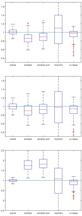
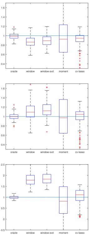
The window size is chosen based on an inflection point in the values of the estimator for a specific set of parameters as the window size varies. Figure 3.1 shows performance for our estimators with window size based on an inflection point, p = 1000. Signal-less (kβk = 0), low SNR (α = 0.1,

kβk = 1), medium SNR (α = 0.1, kβk = 5), high SNR (α = 0.1, kβk = 10) are shown respectively, top to bottom. As we can see in Figure 3.1, the window and window-svd estimators have reasonable performance compared to the cv-LASSO with slightly larger biases. In particular, we do quite well forα = 0.1, β = 1, performing similarly to cv-Lasso, and with a much smaller variance than the method of moments.

Remark 21. We only include results for α = 0.1 because the algorithm per-forms similarly for α ≤ 0.5. Moreover our theory only covers up to roughly

(39)

α = 0.5 for reasonable choices of window size. The performance for dense signal α= 0.9 is covered in its own section below.

3.4.1 Optimal Window Size

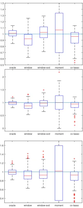
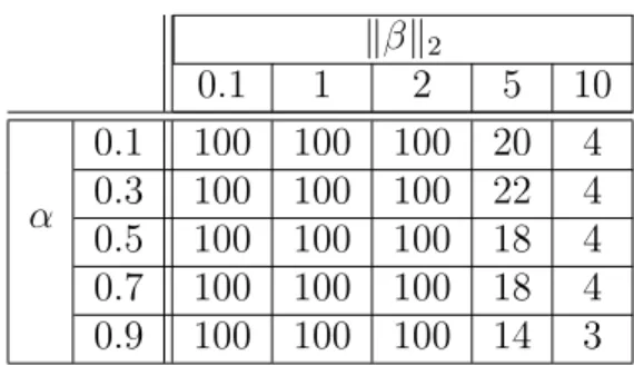
It is notable to see how well our method can perform when the window size is optimized. Here, we give some representative plots (Figure 3.2) to show what happens to performance when replacing the window size with the optimal window size using prior knowledge of the variance. In all experiments, n=100 and p=1000. For the low SNR regimes, we see a similar downward bias to the oblivious choice of window size, although with a smaller bias. Similarly, for high SNR, the upward bias is also smaller than when choosing an oblivious window size. Table 3.1 shows optimal window sizes as a function of α and

kβk2 forp= 200. The optimal window size was found by a grid search over all

possible window sizes using knowledge of the true variance. We note that the optimal window size is generally decreasing as a function of both the signal to noise ratio and the sparsity. Moreover, choosing the maximal window size is optimal in modest regimes.

Figure 3.2 shows the various lasso estimators with optimal window size, p = 1000. Top to bottom: Signal-less (kβk = 0), low SNR (α = 0.1, kβk = 1), high SNR (α= 0.1,kβk= 10) respectively.

(40)

oracle window window-svd moment cv-lasso 0.4 0.6 0.8 1 1.2 1.4 1.6

oracle window window-svd moment cv-lasso -0.5 0 0.5 1 1.5 2 2.5

(41)

oracle window window-svd moment cv-lasso 0.5 0.6 0.7 0.8 0.9 1 1.1 1.2 1.3 1.4 1.5

oracle window window-svd moment cv-lasso 0

0.5 1 1.5 2

(42)

kβk2 0.1 1 2 5 10 α 0.1 100 100 100 20 4 0.3 100 100 100 22 4 0.5 100 100 100 18 4 0.7 100 100 100 18 4 0.9 100 100 100 14 3

Table 3.1: Optimal window sizes as a function of α, kβk2.

3.4.2 High Dimension

In this section we highlight the regime in which our estimator is most useful - whenpnis large. In particular, we chosen= 100,p= 100000 in all experiments. In this regime, it is inefficient to even compute an optimal box size based on an inflection point in the value of the estimator, so instead the choice L = 25 was fixed for all experiments. The results are shown in Figure 3.3, p = 100000 L = 25. Top to bottom: Signal-less (kβk = 0), low SNR (α = 0.1, kβk = 1), high SNR (α = 0.1, kβk = 10) respectively. Although the bias remains, the estimator performs well, especially in low SNR regimes. This is likely due to the strength of the compressed sensing properties for the design matrix as the dimension grows. The bias increases with higher SNR, however our estimator maintains a lower variance than cv-LASSO.

3.4.3 Orthogonal Design Matrix

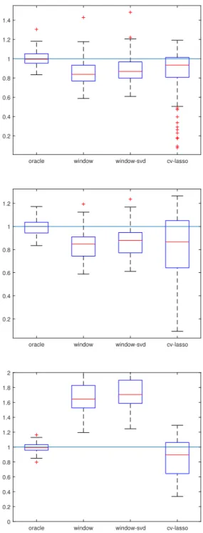
We find our estimator performs quite well in the case where the design matrix is orthogonal, as shown in Figure 3.4, p = n = 200. Top to bottom: Signal-less (kβk = 0), low SNR (α = 0.1, kβk = 1), high SNR (α = 0.1,

(43)

oracle window window-svd cv-lasso 0.2 0.4 0.6 0.8 1 1.2 1.4

oracle window window-svd cv-lasso 0.2 0.4 0.6 0.8 1 1.2

oracle window window-svd cv-lasso 0 0.2 0.4 0.6 0.8 1 1.2 1.4 1.6 1.8 2

(44)

kβk = 10) respectively. In all experiments, the window size is chosen via inflection point in the value of the estimator. The method of moments still performs reasonably well, but suffers a strong upwards bias for large SNR. We note that in all regimes, our estimator performs better than cross-validated LASSO. Moreover, it is more robust to changes in SNR than when the design matrix is RIP (but not necessarily orthogonal).

(45)

0.5 1 1.5

(46)

3.4.4 Dense Signal

Our theory does not cover high sparsity levels (α≥0.9), but nonethe-less our estimator performs well. Although more prone to high levels of SNR, we are still competitive with cv-LASSO in low SNR regimes as seen in Figure 3.5. p = 200, top to bottom: Low SNR (α = 0.9, kβk = 1), medium SNR (α = 0.9,kβk= 5), high SNR (α= 0.9, kβk= 10), respectively.

(47)

oracle window window-svd moment cv-lasso -0.5 0 0.5 1 1.5 2 2.5

(48)

3.5 Real Data

In this section we report results on real data sets well suited for LASSO. Typical data sets where p n involve genetics data, where the amount of genetic data recorded is much larger than the number of patients sampled.

The first data set is from [57] and corresponds to gene expression data. It is presented as a 102x6033 matrix, where each row is a sample from a single subject, and the columns are expression levels. We defer to the original paper for how precisely these values were computed. This data is regressed against a length 102 vector with 52 cancer patient (1) and 50 healthy patients(0). We also consider the well-know Golub data set [27], which is a gene expression data set from subjects with human acute myeloid(AML) and acute lymphoblastic leukemias(ALL). It is represented as 3571 expression levels over 72 patients, with 47 ALL subjects and 25 AML. The final data set is from Alon et al. [5], a 62x2000 matrix of gene expression data from colon tissue, 40 tumor 22 normal. Note that in all cases we have a small number of subjects (< 102) and thousands of gene expressions for each subject.

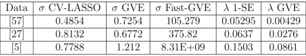
Since we have no knowledge of the true noise of the variance in real world data, we instead compare the noise variance computed for 10 fold CV-LASSO to that of our estimators, as well as the resultingλ parameter. These results are tabulated in table 3.2. We note that with the refined version of our scheme, the estimated variance and resultingλ parameter are close to the correspondingλ value for 1 standard error in CV-LASSO.

(49)

Data σ CV-LASSO σ GVE σ Fast-GVE λ 1-SE λ GVE [57] 0.4854 0.7254 105.279 0.05295 0.00429

[27] 0.8132 0.6772 375.82 0.0637 0.0276

[5] 0.7788 1.212 8.31E+09 0.1503 0.0861

Table 3.2: σ and λ values for real data sets.

We also plot, in figures 3.6-3.8 the corresponding curves for the mean squared error of the LASSO solution, using theλ parameters from table 3.2.

(50)

10-2 10-1 Lambda 0.1 0.12 0.14 0.16 0.18 0.2 0.22 0.24 0.26 MSE

LambdaGVE MSE with Error Bars

LambdaMinMSE Lambda1SE

Figure 3.6: MSE for 10-fold CV LASSO using data from [57], with theλvalue given by the estimator from Algorithm 2 marked in magenta.

3.6 LASSO Proofs

3.6.1 Proof Ingredients

Proposition 22. (Lemma 1 in [39]) SupposeZ has a chi-squared distribution with d degrees of freedom. Then,

Pr[d−2√dt ≤Z ≤d+ 2√dt+ 2t]≥1−2e−t ∀t≥0. (3.3) Proposition 23. (Proposition 2.5 in [52]) Suppose Ωu ∩Ωv = ∅, and that

X ∈ _Rn×p _{satisfies RIP of order} _s

0 and level δ > 0 with s0 = |Ωu|+|Ωv|.

Then,

kX_ΩT_uXΩvk2→2 ≤ √

(51)

10-1 Lambda 0.1 0.12 0.14 0.16 0.18 0.2 0.22 0.24 MSE LambdaGVE

MSE with Error Bars LambdaMinMSE Lambda1SE

(52)

10-1 Lambda 0 0.05 0.1 0.15 0.2 MSE LambdaGVE

MSE with Error Bars LambdaMinMSE Lambda1SE

(53)

Proposition 24. (Equation (5.5) in [63]) Let X be a Gaussian random vari-able with mean 0, variance σ. Then,

Pr[|X|> t]≤2e−t2/2σ2, t ≥1. 3.6.2 Proof of Theorem 16

Consider the window estimators Sj = 1 L X i∈Ωj |yi|2 = 1 L X i∈Ωj |βi+ηi|2 = 1 L X i∈Ωj |βi|2+ 1 L X i∈Ωj |ηi|2+ 2 1 L X i∈Ωj βiηi. Set Ej := _L1 P i∈Ωj|ηi| 2_. _E

j is a sum of L independent squares of N(0, σ2)

random variables. ThenEj concentrates strongly around its expected value,

E(Ej) = σ2.

Note thatEj has a chi-squared distribution with L degrees of freedom, so by

(3.3) with the choicet= log(p)2 _{and after a union bound over all}_p/L_windows,

we get that with probability at least 1−2

p, 1− 5 log(p) σ2 ≤Ej ≤ 1 + 5 log(p) σ2,

holds uniformly for all j ∈ {1,2, . . . , p/L}, assuming that L≥log3(p).

Since L≤ ₂p_s by assumption, the pigeon hole principle implies that at least ₂p_L windows do not overlap Ωβ. On any such “good” window k we have

(54)

kβk:k+L−1k22 = 0 and hence

|Sk−σ2| ≤

5σ2

log(p). (3.5)

Thus, ifSis the average over a subset of the good windows, then also|S−σ2| ≤

5σ2

log(p).

Now, to bound the estimator above on any window, we need some control on the cross term P

i∈Ωjβiηi. Note that this quantity is just a sum

of i.i.d. Gaussians with mean zero and with variance kβΩj∩Ωβk 2

2σ2; thus, by

concentration, we have that with probability at least 1 −2/p, the following holds uniformly over all windows:

X i∈Ωj βiηi ≤ 2σkβΩj∩Ωβk2 p log(p) L . (3.6)

Hence, for any any window, Sj ≥ 1 LkβΩj∩Ωβk 2 2+Ej − 2 L X i∈Ωj∩Ωβ βiηi ≥ 1 LkβΩj∩Ωβk 2 2+ 1− 5 log(p) σ2− kβΩj∩Ωβk2 √ L 2σ√logp √ L ≥ 1− 5 log(p) σ2− σ 2_log(p) L (3.7) ≥ 1− 6 log(p) σ2,

where the final inequality holds because log2(p)≤L. Now, consider the surrogate estimator σc_S2 = 2L

p

Pp/(2L)

j=1 S(j). By

con-struction, cσ2_S ≤ S, where S is the average over any p/(2L) “good” windows.

From the above analysis, we have that with probability exceeding 1− 4

(55)

|σc_S2 −σ2| ≤

6 log(p)σ

2_.

Thus, for our final estimator,σc2

S = (1 + 1 log(p))σb2, we have |σb2−σ2| ≤ 7 log(p) + 6 (log(p))2 σ2 3.6.3 Proof of Theorem 17 Recall that ˜y :=ZT_y _∈

Rp. Consider the window estimate

The first term is small if Ωj and Ωβ have disjoint support, sinceX has the RIP,

the center term gets close to its expectationσ2 due to standard concentration inequalities, and the third term is also small due to standard concentration in-equalities. More concretely, if we assume thatSj is a “good” window, meaning

that Ωj and Ωβ have disjoint support, by equation (3.4)

1 LkX T ΩjXΩββk 2 2 ≤ δkβk2 2 L . (3.9)

(56)

All of the diagonal entries of Σj are in the range [ √ 1−δ,√1 +δ], hence by (3.9) 1 LkZ T ΩjXΩββk 2 2 ≤ 1 +δ L kX T ΩjXΩββk 2 2 ≤ δ(1 +δ)kβk 2 2 L ≤ 2δkβk 2 2 L (3.10)

For the center term, note thatkZΩjηk 2

2 =kPLηk22wherePLis projection

onto the first L coordinates. Next, we know that kPLηk22 has a chi-squared

distribution withL degrees of freedom, so by (3.3) witht = log(p2_),

Prh|kPLηk22−Lσ

2_{| ≤}_2σ2p_L_{log(p) + log(p)}i_≥₁₋ 2

p2.

Hence by a union bound, with probability at least 1− 2

p, the following holds

uniformly over all windows:

|kZ_ΩT jηk 2 2/L−σ 2_|₌_|k_P Lηk22/L−σ 2_| ≤2σ2 r log(p) L + 2σ 2log(p) L ≤ 5σ 2 log(p) (3.11)

For the final term in 3.8, note that _L2 P i∈Ωj(Z

T_Xβ)

i(ZTη)i is a

Gaus-sian random variable with variance 2σkZΩjXββk2/L. Thus, by Proposition 24

(57)

least 1− 1 p: 2 L X i∈Ωj (ZTXβ)i(ZTη)i ≤ 4σkZΩjXββk2 p log(p) L (3.12) ≤ 8 √ δσkβk2 p log(p) L , (3.13)

Thus, averaging over any set of p/2L “good” windows, using (3.10) (3.11) and (3.13) we have 2L p X j Sj−σ2 ≤ 2δkβk 2 2 L + 5σ2 logp+ 8√δσkβk2 √ logp L (3.14)

with probability at least 1− 4

p. Thus, by construction, the estimator σc

2 S = 2L p P jS(j) also satisfies c σ2 S ≤σ 2₊2δkβk22 L + 5σ2 logp + 8√δσkβk2 √ logp L .

It remains to show that the window estimatorσc2

S cannot be too small.

The inequalities (3.12) and (3.11) hold uniformly over all windows, not just good windows; hence, for any window Sj,

Sj ≥ 1 LkZ T ΩjXΩββk 2 2+ 1 LkZ T Ωjηk 2 2− 2 LkZ T ΩjXΩββk2kX T Ωjηk2 ≥ 1 LkX T ΩjXΩββk 2 2+σ 2₋ 5σ2 log(p) − 8σkXT ΩjXΩββk2 √ logp L ≥σ2− 5σ 2 log(p)− 4σ2_log(p) L .

(58)

Combining the bounds, − 5σ 2 log(p) − 4σ2_log(p) L ≤ 2L p X j S(j)−σ2 ≤ 2δkβk 2 2 L + 5σ2 logp+ 8√δσkβk2 √ logp L

For our final estimatorσb2 = (1 + 1

log(p))σc 2 S, we have |σb2−σ2| ≤ (1 + 1 log(p)) 2δkβk 2 L + 6σ2 log(p) + 1 Lmax(4σ 2_log(p),₈√_δσ_k_β_k2p log(p))

(59)

Chapter 4 Locality Sensitive Hashing

This section is based on work that appears in the publication [34]. Nearest neighbor search (NN) is a recently popular task of retrieving the nearest point in some point set to a given query point. The typical regime of this problem is that there are many points and they are in very high dimen-sion. To be more precise: given a metric space (X,D) and a set of pointsP =

{x1, ..., xn} ⊂ X, for a query point x ∈ P find y = argminxi∈P\{x}D(xi, x).

Typically, X = _Rd, Sd−1, or _Fn₂ and D is some `p, cosine similarity, or χ2

distance. The above problem is also known as exact nearest neighbor search, because we want to know the single minimal nearest neighbor inP. In partic-ular, it was shown in [68] that when d is large, popular partioning/clustering techniques are outperformed by brute force search (that is, computing the pairwise distance of every point to the query point).

In order to improve performance, it is often enough in practice to solve an approximate version of nearest neighbor search named (R, c)nearest neighbor search ((R, c)-NN): given a query pointx∈P and the assurance of a point y0 ∈P such that D(y0, x)< R, find y ∈P such that D(y, x) < cR. Note that instead of solving the exact nearest neighbors problem (which

(60)

de-grades to linear search in high dimensions), by solving approximate nearest neighbor search we can achievesublinear query time usinglocality sensitive hashing (LSH). The idea in LSH is to specify a function from the domain X to a discrete set of hash values – ahash function – which sends closer points to the samehash value with higher probability than points which are far apart. Then, for a set of pointsP ={x1, ..., xn} ⊂X and a query pointx∈P,search

within its corresponding hash bucket for a nearest neighbor.

The above discussion begs the obvious question: what makes LSH good for (R, c)-NN, and how can we quantify this? First we need a notion of sensi-tivity for our hash functions.

Definition 25. For r1 ≤ r2 and p2 ≤ p1, a hash family H is (r1, r2, p1, p2

)-sensitive if for all x, y ∈Sd−1,

• If kx−yk2 ≤r1, then PrH[h(x) =h(y)]≥p1.

• If kx−yk2 ≥r2, then PrH[h(x) =h(y)]≤p2.

Intuitively, this measures how often a hash function maps close points to the same value, and far points to different values. The more sensitive a hash function is (i.e. p1 is close to 1, p2 is close to 0 for some fixed r1, r2),

the more effective it should be for the (R, c)-NN problem. We primarily care about the case wherer1 =R, r2 =cR, in which case we study the parameter

ρ= ln(p

−1

1 )

(61)

which quantifies sensitivity. The key result, which directly links the sensitivity of a hash family to how well it performs for (R, c)-NN search is the following (a result of this type first appeared in [31] but we use a more recent version with improved bounds).

Theorem 26. (Theorem 1 in [20]) Given an(R, cR, p1, p2)-sensitive hash

fam-ily H, then there exists an algorithm that solves (R, c)−N N with constant probability, using O(dn+n1+ρ₎_{space, with query time}_O(nρ_{), and}_O(nρ_ln

1/p1n) evaluations of hash functions from H.

The above algorithm stores L hash tables from the family G, where each g ∼G is given by g(x) = (h1(x), ..., hk(x)), and hi ∼ H, i= 1...k. Then,

given a query point x ∈ X, the algorithm looks for collisions in the buckets g1(x), ..., gL(x). The choice of parametersk =nρ,L= ln1/p1n ensure that the algorithm solves (R, c)-NN with constant probability.

4.1 LSH Schemes

It should be clear from above that the correlation between ρ and R is a key feature in determining how effective a hash function is for LSH. To see this in a simple example, consider the hash function for X = _Sd−1_, _D _{is the}

angular distance, defined by

h(x) = sign(hG, xi),

whereG∈_Rd×d_{is a random Gaussian matrix with i.i.d.} _N_(0,_{1) entries}

(62)

SO(d)). This rounding map traces back to Goemans and Williamson [26] and was introduced in the context of LSH by Charikar [17]. It has the advantage of being incredibly easy to implement, however has two main drawbacks: the O(d2_{) matrix/vector multiplication is slow, and it has suboptimal sensitivity.}

To see this, observe that the above hash function is equivalent to if we first project onto a random 2-dimensional hyperplane, then hash to a line with uniformly random angle with the x-axis. We can compute

Pr[h(x) =h(y)] = 1−θ(x, y)/π,

whereθ(x, y) is the angular distance between xand y. Consequently, for this scheme, if kx−yk2 =R and for fixedc >0,

ρ= ln(1−R) ln(1−cR) ≤

1

c. (4.2)

Moreover, ρ ↑ 1

c as R → 0. However, for the case of the unit sphere with

euclidean metric, the optimal sensitivity ρ = _c12 is given in [48]. Spherical lsh ( [8], [9]) has been shown to satisfy this, however the corresponding hash functions are not practical to compute. The work [7] showed the existence of an LSH scheme with optimally sensitive hash functions which are practical to implement; namely, thecross-polytope LSH scheme which has been previously proposed in [58] (see also [10], [48], [46]). Given a Gaussian matrix G∈ _Rd×d

with i.i.d. N(0,1) entries, the cross polytope hash of a point x ∈ Sd−1 is defined as h(x) = argmin u={±ei} Gx kGxk2 −u 2 , (4.3)

(63)

where{ei}di=1 is the standard basis for Rd. Specifically, the name “cross

poly-tope” arises (as with a few other hashing schemes) as the convex hull of the vertex set{±ei}di=1. A recent paper of Andoni, Indyk, Laarhoven, and

Razen-shteyn [7] gives the following collision probability for cross-polytope LSH. Proposition 27 (Theorem 1 in [7]). Suppose x, y ∈Sd−1 _{are such that} _k_x₋

yk2 =R, with 0< R <2, and H is the hash family defined in (4.3). Then,

ln 1 Pr_H[h(x) =h(y)] = R 2 4−R2 lnd+OR(ln(lnd)). (4.4) Consequently, ρ= 1 c2 4−c2R2 4−R2 +o(1).

Remark 28. The above proposition that cross-polytope LSH is asymptotically optimal with respect to ρ. In fact, the coefficient 4₄−₋c2_RR22 < 1 for every choice of c > 1 and 0< R <2, but this does not break the lower bound given in [48] since the lower bound ρ = _c12 only holds for a particular sequence R = R(d). For cross-polytope LSH and the schemes that follow, any sequence R(d) → 0 suffices.

Still, this scheme is limited in efficiency by the O(d2_{) computation}

re-quired to compute a dense matrix-vector multiplication in (4.3). To reduce this computation, [7] proposed to to use a pseudo-random rotation in place of a dense Gaussian matrix, namely,

h(x) = argmin_u₌_{±_e

(64)

whereH ∈_Rd×d _{is a Hadamard matrix and} _D

b, Db0, D_b00 ∈_Rd×d are

indepen-dent diagonal matrices with i.i.d. Rademacher entries on the diagonal. This scheme has the advantage of computing hash functions in timeO(dlnd), and was shown in [7] to empirically exhibit similar collision probabilities to cross-polytope LSH, but provable guarantees on the asymptotic sensitivity of this fast variant of the standard cross-polytope LSH remain open.

4.1.1 Fast cross-polytope LSH with optimal asymptotic sensitivity While we do not prove theoretical guarantees regarding the asymptotic sensitivity of the particular fast variant (4.5), we construct a different variant of the standard cross-polytope LSH (defined below in (4.6)) which also enjoys

O(dlnd) matrix-vector multiplication, and for which we are able to prove optimal asymptotic sensitivity ρ= 1

c2: hF(x) = argmin u={±ei} G(HSDbx) kG(HSDbx)k2 −u 2 ; (4.6)

Here, Db : Rd → Rd is a diagonal matrix with i.i.d. Rademacher entries on

the diagonal,HS ∈Rm×dis a partial Hadamard matrix restricted to a random

subset S ⊂[d] of |S| =m =O(log(d)) rows, and G :_Rm → _Rd0

is a Gaussian matrix that lifts and rotates in dimension d0 in the range m ≤d0 ≤ d. There is nothing special about lifting to dimension d, and indeed one could lift to dimensiond0 > d, but ifd0grows faster thand, the hash computation no longer takes timeO(dlnd).

(65)

trans-form1_{, and embeds the points in dimension} _m_≈_ln_d.

It is straightforward that the hash computation x → hF(x) takes

O(d0m) time from the Gaussian matrix multiplication andO(dlnd) time from the JL transform. We will show that optimal asymptotic sensitivity is still achieved without lifting,d0 =m, but we observe both empirically and theoret-ically that the rate of convergence to the asymptotic sensitivity improves by lifting to higher dimension; takingd0closer todresults in empirically closer re-sults to the standard cross-polytope scheme (see section 4.6 for more details). Moreover, our scheme achieves the lower bound given by Theorem 2 in [7] for the fastest rate of convergence among all hash families which has to d0 values. 4.1.2 Fast cross-polytope LSH with optimal asymptotic sensitivity

and few random bits

Aiming to construct a hash family with similar guarantees which also uses as little randomness as possible, we also consider a discretized version of the fast hashing scheme (4.6) in which the Gaussian matrix G ∈ _Rd0_×_m

is replaced by a matrixGb∈Rd

0_×_m

whose entries are i.i.d. discrete approximations of a Gaussian; in place of the “standard” fast JL transformHSDb, we consider

Z ∈ _Rd×m _{a low-randomness JL transform that we will clarify later. Then,}

the discrete fast hashing scheme we consider is

1_{Formally, given a finite metric space (}_X,_{k · k}₎ _⊂

Rd, a JL transform is a linear map

Φ : Rd →Rm such that for all x∈ X, (1−δ)kxk2 ≤ kΦxk2 ≤(1 +δ)kxk2, with m d

(66)

hD(x) = argmin u={±ei} b G(Zx) kGb(Zx)k₂ −u 2 . (4.7)

Also for this scheme, the hash computation x → h(x) takes O(d0m) time from the Gaussian matrix multiplication and O(dlnd) time from the JL transform. Our scheme has several advantages, due to the fact that the choice of d0 in the range d ≤ d0 ≤ m is flexible: To summarize our main contributions, we prove for both the fast cross-polytope LSH and the fast discrete cross-polytope LSH,

• For eachd0 in the rangem ≤d0 ≤d, this scheme achieves the asymptot-ically optimal ρ. Moreover, ford0 =d, the rate of convergence to this ρ is optimal over all hash families with d hash values.

• With the choice d0 = d, the scheme computes hashes in time O(dlnd) and performs well empirically compared to the standard cross-polytope with dense Gaussian matrix.

• With the choice d0 = m, and by discretizing the Gaussian matrix, we arrive at a scheme that has only O(ln9(d)) bits of randomness and still has optimal asymptotic sensitivity.

Table 4.1 contains the construction of the original cross-polytope LSH scheme, our fast cross-polytope scheme, as well as the discretized version.