A P P L I E D O P T I M I Z AT I O N
Compiled on April 21, 2019
B E N J A M I N PA A S S E N,
A N D R É A R T E LT,
P R O F. B A R B A R A H A M M E R
Faculty of Technology,
Bielefeld University
This script is licensed under the Creative Commons Attribution Share-Alike License Version CC-BY-SA 3.0 (or later). The detailed license text is available athttps://creativecommons.org/licenses/by-sa/3.0/de. This script is based on the brilliant “smart-thesis” template by Andreas Stöckel und Jan Göpfert; usage according to Creative Commons Zero license.
Special thanks go to André Artelt, whose supplementary notes on “Introduction to Machine Learning” formed a firm basis and starting point for this document. Thanks for helpful feedback and comments to Arne Kramer-Sunderbrink and André Artelt.
Change log:
2019-03-26: Adjusted Definitions 15 and 22 slightly to make handling of continuous cases more intuitive. Also made overall notation more consistent.
2019-03-29: Adjusted Definition22 once more.
2019-04-21: Added Section 2.5on heuristics. Revised the entire script and sorted out many minor mistakes.
C O N T E N T S
Contents iv
Introduction vii
1 Theory 1
1.1 Basic Concepts of Optimization . . . 1
1.1.1 Optimization Problems and Formalization . . . 1
1.1.2 Standard Form . . . 5
1.1.3 Global and Local Optima . . . 7
1.1.4 Continuous versus Discrete Optimization Problems . . . 10
1.2 Differentiable Optimization . . . 11
1.2.1 Gradient, Hessian, and Taylor Expansion . . . 11
1.2.2 Searching for Optima with Gradient and Hessian . . . 13
1.2.3 Eigenvalue analysis . . . 15
1.3 Convex Optimization . . . 17
1.3.1 Definition and Convex Optimization Theorem . . . 17
1.3.2 Engineering Convex Problems . . . 19
1.4 Duality . . . 24
1.4.1 Lagrange Dual Form . . . 24
1.4.2 Duality Gaps . . . 25
1.4.3 Karush-Kuhn-Tucker conditions . . . 28
1.4.4 Wolfe Dual Form . . . 31
2 Algorithms 35 2.1 Analytical Methods . . . 35 2.1.1 Unconstrained Optimization . . . 35 2.1.2 Equality-Constrained Optimization . . . 38 2.1.3 Inequality-Constrained Optimization . . . 41 2.2 Numeric Methods. . . 43 2.2.1 Unconstrained Optimization . . . 43 Gradient Descent . . . 43
Stochastic Gradient Descent / Adam . . . 45
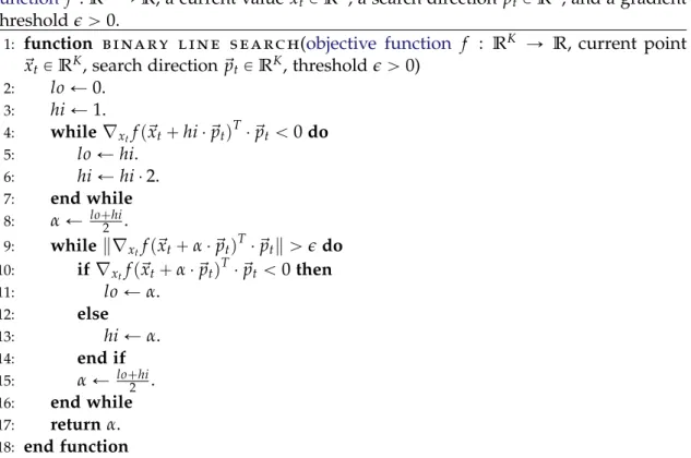
Optimizing the Step Size . . . 46
Conjugate Gradient . . . 49
Newton’s Method . . . 50
(L-)BFGS . . . 52
Trust Region Method. . . 54
2.2.2 Constrained Optimization . . . 57
The Log-Barrier Method . . . 57
Penalty Method . . . 59 Projection Methods . . . 60 2.3 Probabilistic Optimization . . . 65 2.3.1 Maximum Likelihood . . . 65 2.3.2 Maximum a posteriori . . . 66 2.3.3 Expectation Maximization . . . 67
2.3.4 Belief Propagation and Max-Product-Algorithm . . . 73 2.4 Convex Programming . . . 77 2.4.1 Linear Programming . . . 77 2.4.2 Quadratic Programming. . . 77 2.5 Heuristics . . . 80 2.5.1 Gradient-free Optimization . . . 80
Downhill-Simplex / Nelder-Mead algorithm . . . 80
CMA-ES . . . 82 Bayesian Optimization . . . 83 2.5.2 Discrete Optimization . . . 88 Hill Climbing . . . 88 Simulated Annealing . . . 89 Tabu Search . . . 89
Branch and Cut . . . 90
Ant Colony Optimization . . . 91
Bibliography 95
Acronyms 97
Glossary 99
This document is meant to accompany the lecture Applied Optimization at Bielefeld University. It has been first drafted in summer term 2019 and is based on the excellent supplementary notes on “Introduction to Machine Learning” by André Artelt.
Note that this document deviates slightly from the structure of the lecture in that these notes are structured into two chapters, one on theory and one on algorithms. Further, this preliminary version of the lecture notes does not yet contain meta-heuristics or discrete optimization techniques. Further, the algorithmic chapter covers heuristics – namely the the Downhill-Simplex algorithm, Bayesian Optimization, and CMA-ES – in the same chapter as meta-heuristics.
We emphasize that reading this document is no replacement for visiting the lecture and should rather be regarded as an additional learning resource. Further, this document is likely to contain (hopefully minor) errors and mistakes. If you find any of those, please write [email protected].
1
T H E O R YThis chapter covers excerpts of the theory of optimization. Due to the theoretical topics, the structure is more akin to a math textbook, meaning that we feature a series of defini-tions, examples, remarks, and theorems. Still, we will try to add intuitive explanations to all concepts. Therefore, if you are uncertain what a definition or a theorem mean, best look for the explanation or example right after it which hopefully makes it more clear.
1.1 B A S I C C O N C E P T S O F O P T I M I Z AT I O N
In this section, we first introduce what anoptimization problemis, how anyoptimization problem can be re-written into a certain standard form, and how we can solve some continuous optimization problems analytically by relying on first- and second-order conditions.
1.1.1 Optimization Problems and Formalization
Definition 1(Minimization problem, maximization problem, optimization problem). We define aminimization problemas a quartuple consisting of the following elements.
1. a listX1, . . . ,XK of arbitrary sets, which we calldomains,
2. a function f :X1ˆ. . .ˆXKÑR, which we callobjective function,
3. a list of tuples pgl1,g1rq, . . . ,pglm,gmr q, where for all i both gli : X1ˆ. . .ˆXK Ñ R
and gri : X1ˆ. . .ˆXK Ñ R are functions which we call the left-hand-side and right-hand-sideof theithinequality constraintrespectively, and
4. a list of tuples phl1,h1rq, . . . ,phln,hnrq where for all j both hlj : X1ˆ. . .ˆXK Ñ R
and hrj : X1ˆ. . .ˆXK Ñ R are functions which we call the left-hand-side and right-hand-sideof thejequality constraintrespectively.
We denote aminimization problemas follows. min
x1PX1,...,xKPXK
fpx1, . . . ,xKq (1.1)
s.t. glipx1, . . . ,xKq ěgirpx1, . . . ,xKq @iP t1, . . . ,mu hljpx1, . . . ,xKq “hrjpx1, . . . ,xKq @jP t1, . . . ,nu
We define amaximization problemthe same way but denote it as follows. max
x1PX1,...,xKPXK
fpx1, . . . ,xKq (1.2)
s.t. glipx1, . . . ,xKq ěgirpx1, . . . ,xKq @iP t1, . . . ,mu hljpx1, . . . ,xKq “hrjpx1, . . . ,xKq @jP t1, . . . ,nu
Both minimization problems and maximization problems are called optimization problems.
Intuitively, aminimization problemis concerned with finding valuesx1 PX1, . . . ,xK P
XK, such that allequality constraintsandinequality constraintsare fulfilled and such that
fpx1, . . . ,xKqis as small as possible. Conversely, a maximization problem is concerned
with finding valuesx1PX1, . . . ,xKPXK, such that allequality constraintsandinequality constraintsare fulfilled and such that fpx1, . . . ,xKqis as large as possible.
Remark 2 (Formalization, modelling). Note that it is not always easy to translate an intuitiveoptimization problemfrom natural language into the terms of Definition1. We call this translation processformalizationor modelling. Usually, we may lose information in that translation, because we can not incorporate all the details of real life into our
optimization problem. We obtain, instead, a simplifiedmodelof our actual problem. Then, we obtain a solution for our model, and have to translate this solution back to real life.
To formalize an optimization problem, you can take the following questions as a guideline.
1. How manyvariables do I have? How do I denote them? 2. What is thedomainfor each of those variables?
3. What is theobjective function, based on these variables? 4. Do I wish to maximize or minimize theobjective function? 5. What areinequality constraintsfor my problem?
6. What areequality constraintsfor my problem?
Example 3(Optimized tin can). Say you made 1.5 liters of home-made vegan soup for a party and want to transport it to the venue in a can. However, because you are aware of ecological issues you wish to use a can that needs the least amount of material. How does this can need to be shaped?
To model this problem, we follow our recipe above.
1. We first decide to approximate the can with a cylinder. A cylinder can be described by two variables, namely the radius and the height (in centimeters). Let’s denote the radius asr and the height ash.
2. The domain for both our variables are the real numbersR.
3. Our objective function is the ’material need’, which scales with the surface area of the cylinder, including the top and bottom lid. Accordingly, we obtain fpr,hq “
2π¨r¨h`2π¨r2.
4. We wish to minimize the surface area.
5. As inequality constraints, we should restrict both variables to be non-negative because a negative radius or height does not make sense. Further, we should ensure that the can has a volume of at least 1.5 liters. The volume of a cylinder is described by the formulagl1pr,hq “π¨r2¨h. Accordingly, we obtain:
g1lpr,hq “π¨r2¨h g1rpr,hq “1500
gl2pr,hq “r g2rpr,hq “0
6. We have no equality constraints, i.e.n“0.
Our overall minimization problem is thus given as follows. min pr,hqPR2 2π¨r¨h`2π¨r2 (1.3) s.t. π¨r2¨hě1500 r ě0 hě0
Example 4(Minimum cost assignment). Say that we organize a children’s birthday party forKchildren and have packedK bags of sweets with different content. We also have a rough idea about how much each child would like each of the bags and have quantified these preference ratings in aKˆKmatrixR, whererk,l indicates how much childkwould
like bagl. Now we want to find a one-to-one assignment of bags to children, such that the overall enjoyment is maximized.
1. We can frame our variable as a matrix Xwhere xk,l “1 if and only if we give bagl
to child k.
2. The domain for our variable is the space ofKˆKmatrices with binary entries, i.e. X “ t0, 1uKˆK.
3. Our objective function is the ’overall enjoyment’, which we can quantify as follows:
fpXq “řKk“1řKl“1xk,l¨rk,l.
4. We wish to maximize the overall enjoyment. 5. We have no inequality constraints, i.e.m“0.
6. As equality constraints, we wish that every child gets exactly one bag and every bag goes to exactly one child, i.e. we obtain:
hl1pXq “ K ÿ k“1 xk,1 hr1pXq “1 .. . hlKpXq “ K ÿ k“1 xk,K hrKpXq “1 hlK`1pXq “ K ÿ k“1 x1,k hrK`1pXq “1 .. . hl2¨KpXq “ K ÿ k“1 xK,k hr2¨KpXq “1
Our overall maximization problem is given as follows. max XPt0,1uKˆK K ÿ k“1 K ÿ l“1 xk,l¨rk,l (1.4)
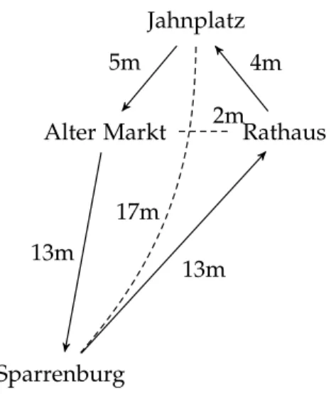
Rathaus Jahnplatz Alter Markt Sparrenburg 4m 5m 13m 13m 17m 2m
Figure 1.1:An instance of the traveling salesperson problem with an optimal round tour, indicated by connecting lines with the travel time in minutes. The travel time for unused connections is annotated with dashed lines
s.t. K ÿ k“1 xk,l “1 @lP t1, . . . ,Ku K ÿ l“1 xk,l “1 @k P t1, . . . ,Ku
Example 5 (Traveling salesperson problem). Say that we wish to see all the beautiful sights of Bielefeld downtown, like the Sparrenburg, the old market, the old city hall, the Leineweber memorial, and so on. Overall, there aremsights we wish to visit. However, we also wish to walk as little as possible. Using the internet, we have researched the time we need to walk from each location to each other location and have recorded these times in amˆmmatrixDwheredi,j is the time we need from locationito location j. Now we
wish to find the shortest round trip. Also refer to Figure1.1.
1. Our variable should be an array~x withmelements, wherext“iindicates that we
visit locationiin thetth step of our journey.
2. The domain for our variable is the set of all possible permutations over the set
t1, . . . ,mu, which we denote asX “Πpt1, . . . ,muq.
3. Our objective function is the overall time we need for our round trip, which we can quantify as fp~xq “řmt“´11dxt,xt`1`dxm,x1.
4. We wish to minimize the time we need. 5. We have no inequality constraints. 6. We have no equality constraints.
Our overall minimization problem is given as follows. min ~xPΠpt1,...,muq m´1 ÿ t“1 dxt,xt`1`dxm,x1 (1.5)
Note that we could also have formalized this problem differently, e.g. with a matrix variable like in Example4.
Remark 6 (Domain and constraints). Note that adding constraints to the problem is equivalent to restricting the domain (also refer to the notion of a feasible setlater on). As such, one could argue that constraints are superfluous and we should just specify the domain as a precise set. However, for many practical problems, solutions become much more obvious if we permit a domain that is as general as possible and consider only special kinds of constraints which are easy to handle.
1.1.2 Standard Form
For our subsequent theory it would be increasingly unwieldy to always distinguish be-tween minimization and maximization problems and consider left- and right-hand sides of constraints separately. Therefore, we introduce thestandard form, which is considerably simpler but is still expressive enough to capture all possible optimization problems. Definition 7 (Standard form). We define an optimization problem in standard form as a quartuple with the following ingredients.
1. a single setX, which we calldomain,
2. a function f :X ÑR, which we callobjective function,
3. a listg1, . . . ,gmof functionsgi :X ÑR, which we callinequality constraintfunctions,
and
4. a listh1, . . . ,hn of functionshj :X ÑR, which we callequality constraintfunctions.
We denote an optimization problem in standard form as follows. min xPX fpxq (1.6) s.t. gipxq ě0 @iP t1, . . . ,mu hjpxq “0 @jP t1, . . . ,nu Now, let min x1PX1,...,xKPXK fpx1, . . . ,xKq (1.7) s.t. glipx1, . . . ,xKq ěgirpx1, . . . ,xKq @iP t1, . . . ,mu hljpx1, . . . ,xKq “hrjpx1, . . . ,xKq @jP t1, . . . ,nu
be aminimization problemand let min px1,...,xKqPX1ˆ...ˆXK ˜ fpxq (1.8) s.t. g˜ipxq ě0 @iP t1, . . . ,mu ˜ hjpxq “0 @jP t1, . . . ,nu
be an optimization problem in standard form. We call 1.7 and 1.8 equivalent if the following conditions hold for allpx1, . . . ,xKq,py1, . . . ,yKq PX1ˆ. . .ˆXK.
glipx1, . . . ,xKq “gripx1, . . . ,xKq ðñ g˜ipx1, . . . ,xKq “0 (1.10) hljpx1, . . . ,xKq “hrjpx1, . . . ,xKq ðñ h˜jpx1, . . . ,xKq “0 (1.11) Now, let max x1PX1,...,xKPXK fpx1, . . . ,xKq (1.12) s.t. glipx1, . . . ,xKq ěgirpx1, . . . ,xKq @iP t1, . . . ,mu hljpx1, . . . ,xKq “hrjpx1, . . . ,xKq @jP t1, . . . ,nu
be amaximization problem. We call1.12and1.8equivalent if the following conditions hold for allpx1, . . . ,xKq,py1, . . . ,yKq PX1ˆ. . .ˆXK.
fpx1, . . . ,xKq ě fpy1, . . . ,yKq ðñ f˜px1, . . . ,xKq ď f˜py1, . . . ,yKq (1.13) glipx1, . . . ,xKq “gripx1, . . . ,xKq ðñ g˜ipx1, . . . ,xKq “0 (1.14) hljpx1, . . . ,xKq “hrjpx1, . . . ,xKq ðñ h˜jpx1, . . . ,xKq “0 (1.15)
Theorem 8(Universality of standard form). Let
min{maxx1PX1,...,xKPXK fpx1, . . . ,xKq (1.16)
s.t. glipx1, . . . ,xKq ěgirpx1, . . . ,xKq @iP t1, . . . ,mu hljpx1, . . . ,xKq “hrjpx1, . . . ,xKq @jP t1, . . . ,nu be an optimization problem. Then, the following optimization problem in standard form is equiv-alent. min px1,...,xKqPX1ˆ...ˆXK ˘fpxq (1.17) s.t. glipxq ´girpxq ě0 @iP t1, . . . ,mu hljpxq ´hrjpxq “0 @jP t1, . . . ,nu
where theobjective functionis just fpxqif the original problem was aminimization problemand
´fpxqif the original problem was amaximization problem.
Proof. First, consider the case where the original problem was aminimization problem. Then, Condition 1.9 is obvious because the objective functions are the same. Condi-tions 1.10 and 1.11 are obvious by simply subtracting the right-hand side from the inequality/equation.
Second, consider the case where the original problem was amaximization problem. Then, Condition1.13follows by multiplying the inequality fpxq ě fpyq with´1. Con-ditions 1.14 and 1.15 are obvious by simply subtracting the right-hand side from the inequality/equation.
Remark 9(Using the standard form). We have motivated the standard form because it makes theoretical arguments easier – whatever we can prove for the standard form automatically applies to alloptimization problems. However, the standard form is also useful in practice because most programming libraries for optimization use this standard form or a related form as an input interface. Therefore, being able to convert from any model to the standard form is a useful skill to have.
Example 10 (Standard forms). The standard form for the tin can problem from Equa-tion1.3is as follows. min pr,hqPR2 2π¨r¨h`2π¨r 2 s.t. π¨r2¨h´1500ě0 rě0 hě0
The standard form for the minimum cost assignment problem from Equation1.4is as follows. min XPt0,1uKˆK K ÿ k“1 K ÿ l“1 xk,l¨ p´rk,lq s.t. K ÿ k“1 xk,l´1“0 @lP t1, . . . ,Ku K ÿ l“1 xk,l´1“0 @k P t1, . . . ,Ku
The traveling Salesperson problem1.5is already in standard form. 1.1.3 Global and Local Optima
Until now we have defined what anoptimization problemis, but we have not yet defined what it means tosolveanoptimization problem. We introduce the concept of a solution now.
Definition 11 (Feasible set, global minimum, solution). We define thefeasible setX˚of
anoptimization problemin standard form as the set X˚ : “ ! xPX ˇ ˇ ˇ@iP t1, . . .mu: gipxq ě0,@jP t1, . . . ,nu:hjpxq “0 ) (1.18) We define aglobal minimumorsolutionof anoptimization problemin standard form as an element x˚ PX˚ such that for allxPX˚ it holds:
fpx˚q ď fpxq (1.19)
Example 12(Logical and). Consider the following optimization problem: min
px,yqPt0,1u2´x¨y (1.20)
Thefeasible setof this problem is the entiredomain, i.e.X˚
“ tp0, 0q,p0, 1q,p1, 0q,p1, 1qu. The former three values have anobjective functionvalue of 0, the last one a value of´1. Accordingly,px,yq “ p1, 1q is theglobal minimumor solution of this problem because
there is no other point in thefeasible setwith a smallerobjective functionvalue.
Remark 13(Equivalence of solutions). It is straightforward to extend Definition 11to generaloptimization problemsand to show that any solution of a generaloptimization problem is also the solution of its equivalentoptimization problemin standard form according to Theorem8and vice versa. For brevity, we omit this here.
Remark 14(Multiple solutions). Note that Definition11does permit multiple solutions. As an example, consider the trivial optimization problem
min
xPR 0
All xPRareglobal minimaof this problem.
Definition 15(Neighborhoods and local minima). LetX be thedomainandX˚ be the feasible setof anoptimization problemin standard form. We call a functionN : X Ñ PpXqaneighborhood functionand we callNpxqtheneighborhoodofx according toN.
We define alocal minimumof anoptimization problem in standard form with respect to the neighborhood functionN as an elementx˚
PX˚ such that it holds:
fpx˚q ď fpxq @xPNpx˚q XX˚ (1.21)
Example 16(Bit-flip neighborhood). Consider the following optimization problem: min
px,yqPt0,1u2
´x¨y
And consider the neighborhood function Npx,yq :“ tp1´x,yq,px, 1´yqu, i.e. the x/y
combinations that result by flipping one bit.
According to that neighborhood function, theglobal minimump1, 1qhas the neigh-borhoodNp1, 1q “ tp0, 1q,p1, 0qu. Both entries have a largerobjective functionvalue, such
that theglobal minimumis also alocal minimumaccording toN.
Now, consider the point p0, 0q. The neighborhood is Np0, 0q “ tp0, 1q,p1, 0qu. Both entries have anobjective functionvalue of 0, which is the same as theobjective function
value ofp0, 0q. Therefore,p0, 0qis also alocal minimumaccording to N, even though it is not aglobal minimum.
Example 17 (Swap neighborhood). Consider the Traveling Salesperson-Problem from Equation1.5for the distances in Figure1.1. For this problem, we can define the neigh-borhood function
Npx1,x2,x3,x4q “ tpx2,x1,x3,x4q,px1,x3,x2,x4q,px1,x2,x4,x3q,px4,x2,x3,x1qu
i.e. we swap a neighboring location in the tour.
According to that neighborhood function, the tour (Jahnplatz, Sparrenburg, Alter Markt, Rathaus) isnotalocal minimum, because we can improve it by swapping Spar-renburg and Alter Markt, which yields aglobal minimum. Thisglobal minimumis also alocal minimumbecause any swap will increase our travel time.
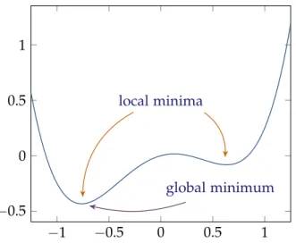
Example 18(Continuous neighborhood). Consider the optimization problem min
xPR x 4
´x2`1
4x for which theobjective functionis shown in Figure1.2.
We define the neighborhood function Nepxq “ yPR
ˇ
ˇkx´ykďe (
(1.22) i.e. thee-ball aroundx.
For e“0.5, x«0.63 is alocal minimumbut not aglobal minimumand x« ´0.76 is both alocal minimumand aglobal minimum.
´1 ´0.5 0 0.5 1 ´0.5 0 0.5 1 local minima global minimum
Figure 1.2:A plot of the function fpxq “x4´x2`14xwith twolocal minimaatx « ´0.76 and
x«0.63, the former one also being aglobal minimum.
Remark 19(Optimization via neighborhood search). Neighborhood functions directly give us a straightforward tool to solve optimization problems. We simply start at a random point in the feasible set, evaluate the objective function for that point, then compute the neighborhood for the point and evaluate theobjective functionfor all points within the neighborhood. If any of these points has a lowerobjective function value, we switch to that point. If no neighbor has a betterobjective function value, we stop. Note that we stop only if we have found a local minimum. Also refer to the optimization method ofhill climbing(Section2.5.2).
Consider Example 16 again. If we start off with x “ p1, 0q, the neighborhood is Np1, 0q “ tp0, 0q,p1, 1qu. We obtain theobjective functionvalues fp1, 0q “0, fp0, 0q “0 and fp1, 1q “ ´1. Therefore, we switch tox “ p1, 1q. All neighbors of x“ p1, 1qhave a higher objective function value, therefore we stop.
Theorem 20 (Relationship of local and global optima). Aglobal minimum is also a local minimumaccording to every neighborhood functionN.
Conversely, not everylocal minimumis aglobal minimum.
Proof. Regarding the first claim, recall the definition of a global minimum. A global minimumis a point x˚
PX˚ such that fpx˚q ď fpxqfor all xPX˚. Then, in particular,
fpx˚
q ď fpxqfor all xin any subset ofX˚. Therefore, irrespective of the neighborhood
function,x˚ is alocal minimum.
The second claim holds because we have provided counterexamples above.
Remark 21 (Intuition behind local minima). When we use the term local minima, we typically refer tolocal minimathat arenotat the same timeglobal minima. These “nasty”
local minimaare particularly interesting because they can easily mislead an optimization algorithm that is based on neighborhoods. For example, if we apply neighborhood search on Example16starting from point x“ p0, 0q, then we immediately stop, even though we have not found aglobal minimumyet.
Therefore, solving problems with manylocal minimathat are notglobal minimais more difficult than solving problems with only a single local minimumwhich is also the
1.1.4 Continuous versus Discrete Optimization Problems
A fundamental distinction in optimization is between continuous and discrete opti-mization. Intuitively, continuous optimization is about smoothobjective functionsand gap-freefeasible sets, whereas discrete optimization is concerned withfeasible setswith gaps and non-differentiableobjective functionswith sudden jumps.
Due to these fundamental differences, the optimization strategies we have to em-ploy are fundamentally different as well. In continuous optimization, we can smoothly move through space and observe a continuous change in theobjective functionvalue corresponding to our movement. In discrete optimization, we have to perform “jumps” through thefeasible set, which we have to control by means of some heuristic.
More formally, we provide the following definition.
Definition 22(Continuous function, continuous optimization problem, discrete optimiza-tion problem). Let f be a function f :RK ÑRfor some KPN. We call f a continuous functionif for all~x PX and alleą0 there exists aδ ą0 such that for all~y PNδp~xq it
holds|fp~yq ´fp~xq| ăe, whereNδ refers to the neighborhood in Equation1.22.
We call anoptimization problemcontinuousif 1. thedomainisX “RKfor someKPN,
2. theobjective function f is a continuous function on thefeasible setX˚,
3. the feasible set is path-connected, i.e. for any two points~x,~y P X˚ there exists a continuous functionφ:r0, 1s ÑX˚, such thatφp0q “~xandφp1q “~y.
We call anoptimization problemdiscreteif thedomainX is countable, i.e. there exists a surjective mappingπ :NÑX.
Example 23 (Continuous and discrete problems). From our previous examples, the tin can problem (Example3) and Example 18are continuous and the minimum cost assignment problem (Example4), the traveling salesperson problem (Example5), and the logical and problem (Example1.20) are discrete.
Remark 24(Beyond continuous and discrete). Note that there existoptimization prob-lemswhich areneithercontinuous nor discrete according to Definition22. Consider the following example.
min
xPR x 2
s.t. |x| ě1
Thefeasible setisp´8,´1s Y r1,8q, which is neither path-connected - because there is a gap between´1 and 1 - nor is it countable. Therefore, this problem is neither continuous
nor discrete.
Some of these more exotic cases can still be addressed with the methods of this course, but we will generally assume that our problems are either discrete or continuous in the sense above.
1.2 D I F F E R E N T I A B L E O P T I M I Z AT I O N
If theobjective functionof an optimization problem is continuous and differentiable, but even we can apply the usual optimization machinery that we know from school: Setting the first derivative to zero and checking the second derivative. In this section, we will try to explain why this machinery works and generalize it to multiple dimensions.
1.2.1 Gradient, Hessian, and Taylor Expansion
The first thing we introduce is a generalization of the first and second derivative to higher dimensions by means of the gradientand theHessianrespectively.
Definition 25 (Gradient and Hessian). Let f be a function f :RK ÑRfor someKPN.
Then, we define thegradientof f at position~xPRk as follows:
∇~xfp~xq “ ¨ ˚ ˝ B Bx1 fp~xq .. . B BxKfp~xq ˛ ‹ ‚ (1.23)
We define theHessianof f at position~xPRk as follows:
∇2 ~xfp~xq “ ¨ ˚ ˚ ˝ B2 B2x1fp~xq . . . B2 Bx1BxK fp~xq .. . . .. ... B2 BxKBx1 fp~xq . . . B2 B2xKfp~xq ˛ ‹ ‹ ‚ (1.24)
The reason why gradient and Hessian are so useful for optimization is because they allow us to indirectly characterize how a objective functionbehaves without having to regard the precise shape of the objective function. Our central tool in that regard is the
Taylor expansion.
Definition 26 (Taylor expansion). Let f :RK ÑRbe a twice-differentiable function.
We define the first-order Taylor expansion of f around some point~x˚ PRK as the
function ˜f1
~x˚ :RKÑRwith the following form.
˜
f~x1˚p~xq:“ fp~x˚q ` p~x´~x˚q
T
¨∇~xfp~x˚q (1.25)
We define the second-order Taylor expansion of f around some point~x˚PRK as the
function ˜f2
~x˚ :RKÑRwith the following form.
˜ f~x2˚p~xq:“ f˜~x1˚p~xq ` 1 2p~x´~x ˚ qT¨∇2~xfp~x˚q ¨ p~x´~x˚q (1.26)
Theorem 27(Taylor’s theorem (excerpt)). Let f :RKÑRbe a twice-differentiable function. For every~x˚
PRK and everyeą0there exists aδą0such that for all~xPNδp~x˚qit holds: |f˜~x2˚p~xq ´ fp~xq| ă |f˜~x1˚p~xq ´ fp~xq| ăe
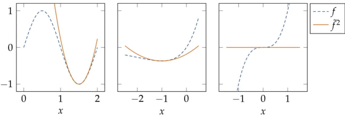
0 1 2 ´1 0 1 x ´2 ´1 0 x ´1 0 1 x f ˜ f2
Figure 1.3:The second-order Taylor approximation of the functions fpxq “sinpπ¨xq, fpxq “
x¨exppxq, and fpxq “x3at positions 1.5,´1 and 0 respectively. The original function is shown as a dashed blue line and the second-order approximation is shown in orange.
Remark 28(Intuition behind the Taylor expansion). The previous theorem tells us that the Taylor expansion is a good approximation if we stay in a small δ-neighborhood
around our point~x˚ and that the second-order approximation is better than the
first-order approximation. Why is that? Intuitively, if a function is continuous, then it changes only a little if we change the input a little, and we can approximate this small change by approximating the function with a tangent. This tangent is described exactly by the first-order Taylor expansion.
The first-order approximation is only inaccurate if the slope changes, i.e. if the first derivative is not constant. However, the first derivative is also a continuous function, which means that the slope changes only slightly if we change the input slightly, such that the approximation is accurate if we stay close enough to~x˚.
The second-order approximation is better because it can even approximate constant changes in slope, i.e. a constant second derivative. If the second derivative is not constant, its change will also only change a little if we stay close to to~x˚ and our second-order
approximation is good if we stay close enough.
An illustration of the second-order Taylor expansion is also visible in Figure1.3. To prove that we can find local minimavia the gradient and the Hessian, we only require one final piece of the puzzle, namely the notion ofpositive definiteness, which will tell us that the curvature around a point is positive.
Definition 29 (Positive (semi-)definiteness). A symmetric square matrix A P RKˆK is calledpositive definiteif for all vectors~xPRKwith~x‰~0 it holds:
~xT¨A¨~xą0 (1.27)
A symmetric square matrix APRKˆK is calledpositive semi-definiteof for all vectors
~xPRK it holds:
~xT¨A¨~xě0 (1.28)
Remark 30(Positive definiteness versus positiveness). Importantly, positive definiteness isnotthe same as having positive entries. Consider the matrices
A1 “ ˆ 1 2 2 1 ˙ and A2“ ˆ 5 ´1 ´1 1.25 ˙ .
A1has only positive entries. However, the vector~x“ p´1, 1qT yields p´1, 1q ¨ ˆ 1 2 2 1 ˙ ¨ ˆ ´1 1 ˙ “ p´1`2,´2`1q ¨ ˆ ´1 1 ˙ “ ´2ă0,
which means thatA1 isneitherpositive semi-definitenorpositive definite.
Conversely, A2 is indeedpositive definite(andpositive semi-definite) even though
it contains negative entries. We will show later in Theorem 35how to check positive definiteness in practice.
1.2.2 Searching for Optima with Gradient and Hessian
We now go on to show that we can findlocal minimaby searching for locations with zero gradient andpositive definiteHessian.
Theorem 31(First- and second-order conditions forlocal minima). Let f : RK Ñ Rbe
a twice differentiable function and consider the unconstrainedoptimization problemin standard form:
min
~xPRK fp~xq
Then it holds for any~x˚
PRK:
1. If∇~xfp~x˚q ‰0, then~x˚ isnotalocal minimum.
2. If∇~xfp~x˚q “~0and∇~2xfp~x˚qispositive definite, then~x˚isalocal minimum.
3. If∇~xfp~x˚q “~0and∇2
~xfp~x˚qisnotpositive semi-definite, then~x˚isnotalocal minimum. 4. If~x˚isalocal minimum, then∇
~xfp~x˚q “~0and∇2~xfp~x˚qispositive semi-definite. Proof. Note that we only provide a sketch of the proof here. The precise version would require to ensure that the approximation error of the Taylor expansions stays within certain bounds, which we omit here.
We consider each claim in turn.
1. This follows from the first-order Taylor approximation, i.e. ˜f~x1˚p~xq “ fp~x˚q `
p~x´~x˚qT¨∇~xfp~x˚q. If the gradient is nonzero, consider the point ~x “ ~x˚´e¨
∇~xfp~x˚qfor a sufficiently smallesuch that the first-order Taylor approximation is
accurate. Then it holds
fp~xq “ f˜~x1˚p~xq “ fp~x˚q ´e¨∇~xfp~x˚qT¨∇~xfp~x˚q ă fp~x˚q.
Therefore, for anyδ ą0, there is at least one point~x PNδp~x˚qwith fp~xq ă fp~x˚q.
This, in turn, implies that~x˚is not alocal minimum.
2. This follows from the second-order Taylor approximation, i.e. ˜f~x2˚p~xq “ fp~x˚q `
1
2p~x´~x˚q T
¨∇~2xfp~x˚q ¨ p~x´~x˚q. Note that the gradient term is removed because the
gradient is zero in this case. Now, consider aneą0 sufficiently small such that this approximation is accurate. Then, because the Hessian ispositive definite, it holds for any~xPNep~x˚qwith~x‰~x˚:
fp~xq “ f˜~x2˚p~xq “ fp~x˚q ` 1 2p~x´~x ˚ qT¨∇~2xfp~x˚ q ¨ p~x´~x˚ q ą fp~x˚ q, such that~x˚ is alocal minimum.
3. This follows again from the second-order Taylor approximation. Because the Hes-sian is not positive semi-definite, there must exist a vector ~y P RK such that
~yT¨∇~2xfp~x˚q ¨~y ă 0. Then, consider the vector~x :“ ~x˚`
e¨ k~~yyk. Note that this vector is guaranteed to lie in thee-neighborhood of~x˚ because
k~x´~x˚k“ke¨ ~y k~ykk“ e k~yk¨k~yk“e Further it holds: p~x´~x˚qT¨∇~2xfp~x˚q ¨ p~x´~x˚q “ pe¨ ~y k~ykq T ¨∇~2xfp~x˚q ¨ pe¨ ~y k~ykq “ e2 k~yk2¨~y T ¨∇~2xfp~x˚q ¨~yă0
Accordingly, for any sufficiently small e such that the second-order Taylor
ap-proximation is accurate it holds: There exists a point ~x :“ ~x˚`e¨ k~~yyk in the e-neighborhood of~x˚such that
fp~xq “ f˜~x2˚p~xq “ fp~x˚q `
1 2p~x´~x
˚
qT¨∇2~xfp~x˚q ¨ p~x´~x˚q ă fp~x˚q
which implies that~x˚ isnotalocal minimum.
4. Follows from the negation of 1. and 3.
Remark 32(Searching forlocal minimavia Theorem31). Theorem31gives us a way to hunt forlocal minimaby setting the gradient to zero and inspecting the Hessian for the resulting solutions – just as we learned in school. It is valuable to inspect the pitfalls of this method, though.
First, we can only apply this method if ouroptimization problemisunconstrained. Second, it isnotsufficient that the Hessian ispositive semi-definite. We needstrict positive definiteness. Otherwise, our point could be either a local minimum, a local maximum, or a saddle point because the function may still be “curved”, albeit in higher-order terms which our second-higher-order Taylor expansion can not “see”. Also refer to the following examples.
Third, we need to check positive definiteness instead of just positive entries. The effective way of doing so is via the eigenvalues, as we will see in Theorem35.
Example 33(Local minimaand Taylor approximation). Consider the examples shown in Figure1.3.
1. Consider fpxq “sinpπ¨xq. Then, we obtain ∇xfpxq “cospπ¨xq ¨πand∇2xfpxq “ ´sinpπ¨xq ¨π2. The gradient is zero for any x˚ P t0.5`k|k PZu. First, consider
x˚P t0.5`2k|kPZu. For these points, we obtain∇2
xfpx˚q “ ´sinpπ¨ r0.5`2ksq ¨ π2“ ´π2 ă0, i.e. our Hessian is notpositive semi-definiteand these points are definitely notlocal minima. Next, considerx˚
P t1.5`2k|kPZu. For these points, we obtain∇2
xfpx˚q “ ´sinpπ¨ r1.5`2ksq ¨π2“π2ą0, i.e. our Hessian ispositive definiteand these points are definitelylocal minima(as visible in Figure1.3, left). 2. Consider fpxq “x¨exppxq. Then, we obtain∇xfpxq “exppxq ¨ p1`xqand∇2
xfpxq “
exppxq ¨ p2`xq. The gradient is zero forx˚
“ ´1. We obtain the Hessian∇2
xfpx˚q “
expp´1q ¨ p2´1q “expp´1q ą0, i.e. our Hessian ispositive definiteand this point is definitely alocal minimum(as visible in Figure1.3, center).
3. Consider fpxq “ x3. Then, we obtain ∇xfpxq “ 3¨x2 and ∇2xfpxq “ 6¨x. The
gradient is zero forx˚“0. We obtain the Hessian∇2
xfpx˚q “0, i.e. our Hessian is positive semi-definite. Still, this point is clearly not alocal minimum(as visible in Figure1.3, right).
In addition, consider the following examples.
1. Consider fpxq “ x4. Then, we obtain ∇xfpxq “ 4¨x3 and ∇2xfpxq “ 12¨x2. The
gradient is zero forx˚
“0. We obtain the Hessian∇2
xfpx˚q “0, i.e. our Hessian is positive semi-definite. Still, this point is aglobal minimumbecause for any xPR
we have fpxq “x4 ě0“ fp~x˚q.
2. Consider fpxq “ ´x4. Then, we obtain ∇xfpxq “ ´4¨x3 and ∇2
xfpxq “ ´12¨x2.
The gradient is zero forx˚
“0. We obtain the Hessian∇2xfpx˚q “0, i.e. our Hessian
ispositive semi-definite. However, out point is indeed a global maximum because for any xPRwe have fpxq “ ´x4ď0“ fpx˚q.
Finally, consider the two-dimensional function fpx,yq “ x2´y2. In this case, we
obtain ∇px,yqfpx,yq “ ˆ 2x ´2y ˙ and ∇2px,yqfpx,yq “ ˆ 2 0 0 ´2 ˙ . The gradient is zero for~x˚
“ p0, 0qT. The Hessian is notpositive semi-definitebecause we find that for~y“ p0, 1qT we obtain
p0, 1q ¨ ˆ 2 0 0 ´2 ˙ ¨ ˆ 0 1 ˙ “ p0,´2q ¨ ˆ 0 1 ˙ “ ´2ă0
Therefore,~x˚ isnotalocal minimum.
1.2.3 Eigenvalue analysis
Until now we are missing an efficient way to check whether a matrix ispositive definite
or positive semi-definite. As it turns out, the key to such a method areeigenvalues. Remark 34 (Refresher: Eigenvalues). As a refresher: An eigenvector of a matrix A is defined as a vector~v‰~0, such that
A¨~v“λ¨~v (1.29)
whereλPRis called theeigenvaluecorresponding to the eigenvector~v. Note that if~vis an eigenvalue of A, thenα¨~vfor anyα‰0 is also an eigenvector of Awith the same eigenvalue.
Further, we can re-write any symmetric square matrixAPRKˆK as follows.
A“V¨Λ¨VT (1.30)
whereV contains eigenvectors ofAas columns andΛis a diagonal matrix containing the corresponding eigenvalues. This form is also called the eigendecompositionofAand can be computed in OpK3q. A special property of this eigenvalue decomposition is that the eigenvectors are orthogonal, that is: V ¨VT “ VT¨V “ IK, where IK is the KˆK-dimensional identity matrix.
With this knowledge in mind, we can now go on to prove that knowing the eigenvalues of Ais sufficient to know its definiteness.
Theorem 35(Positive definiteness and eigenvalues). A symmetric square matrixAPRKˆK
ispositive definiteif and only if all of its eigenvalues are positive.
A symmetric square matrix A P RKˆK is positive semi-definite if and only if all of its eigenvalues are non-negative.
Proof. Since Ais symmetric and square, the eigenvalue decomposition of Ahas the form A“V¨Λ¨VT with V¨VT “VT¨V “IK.
We first prove the second claim.
If all eigenvalues are non-negative, we can re-write Λas?ΛT¨?Λwhere?¨denotes
the element-wise square root. Accordingly, we can re-write for all~xPRK:
~xT¨A¨~x“~xT¨V¨ ? ΛT¨ ? Λ¨VT¨~x“ p ? Λ¨VT¨~xqT¨ p ? Λ¨VT¨~xq ě0, which means that Aispositive semi-definite.
Conversely, if there exists a negative eigenvalue of A, sayλk ă0, then we can consider thekth eigenvector~vk and the product
~vTk ¨A¨~vk “~vTk ¨λk¨~vk“λk ă0
which means that Aisnotpositive semi-definite.
Now, consider the first claim. If all eigenvalues are positive, then?Λ¨VT¨~xis nonzero if~x is nonzero. Therefore, for any nonzero~xwe obtain
~xT¨A¨~x“ p?Λ¨VT¨~xqT¨ p?Λ¨VT¨~xq ą0, which means that Aispositive definite.
Conversely, consider the case of a non-positive eigenvalueλk. Ifλk ă0, then Ais not
evenpositive semi-definite, which means that it is also notpositive definite (see above). ifλk “0 then consider the product
~vTk ¨A¨~vk “~vTk ¨λk¨~vk “0
which means that Aisnotpositive definite.
Remark 36(Eigenvalues of the Hessian and curvature). Intuitively, the eigenvalues of the Hessian specify the curvature of the function along the direction of the corresponding eigenvectors. Positive eigenvalues correspond to upwards curvature, negative eigenvalues to downwareds curvature.
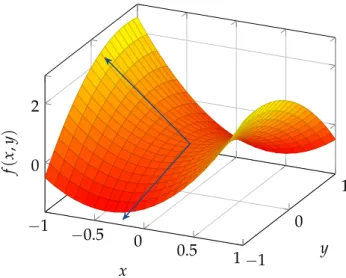
If the curvature along all directions is upwards - that is, if all eigenvalues of the Hessian are positive - we can only increase theobjective functionif we move. However, if even one eigenvalue is negative (or zero), we can move into that direction and decrease the objective function (refer to Figure1.4).
Note that this interpretationonlyapplies for points where the gradient is zero. In other points, the eigenvalues donotcorrespond to curvature. Also note that this interpretation only holds forquadraticcurvature. Higher-order curvatures are not included.
In this section, we have demonstrated how we can findlocal minimain continuous optimization. This begs the question: Under which circumstances can we guarantee that
local minimaare alsoglobal minima? In this regard, a subclass of continuous optimization problems comes into play, namely the class ofconvexoptimization problems.
´1 ´0.5 0 0.5 1 ´1 0 1 0 2 x y f p x , y q
Figure 1.4: An illustration of curvature at a point with zero gradient. The function here is
fpx,yq “2x2´32x¨y´y2, indicated by the surface plot. The arrows indicate the eigenvectors of the Hessian at pointp0, 0q, where thezcoordinate indicates the (square root of) the corresponding eigenvalue. Note that the eigenvalues correspond to the curvature around this point, being positive for upward and negative for downward curvature.
1.3 C O N V E X O P T I M I Z AT I O N
ConvexOptimization is concerned with problems that adhere to certain geometric con-straints (namely convexity). Why do we care about such geometric concon-straints? Because they guarantee a very useful property for optimization, namely that all local minimaare
global minima. Since findinglocal minimais usually easy in continuous optimization (see previous section), having this property makes optimization easy. Accordingly, it is very desirable to re-phraseoptimization problemsinconvexform.
1.3.1 Definition and Convex Optimization Theorem
In this section, we will define precisely what convexity means and then prove thatlocal minimaare global minimaforconvexproblems.
Definition 37 (Convex set, convex function, convexoptimization problem). LetX ĎRK
for someKPN. We call X aconvexsetif for all~x,~yPX and all αP r0, 1sit holds:
α¨~y` p1´αq ¨~xPX. (1.31)
Let f be a function f :X ÑR. We call f aconvexfunctionifX isconvexand for all
~x,~yPX and all αP r0, 1sit holds:
f`α¨~y` p1´αq ¨~x˘ďα¨fp~yq ` p1´αq ¨ fp~xq. (1.32) Finally, consider a optimization problem in standard form. We call this problem
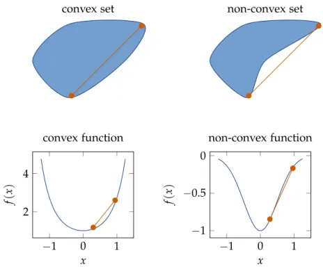
convex set non-convex set ´1 0 1 2 4 x f p x q convex function ´1 0 1 ´1 ´0.5 0 x f p x q non-convex function
Figure 1.5:Top left: A convex set where every connecting line lies in the set; top right: a non-convex set due to two points for which the connecting line doesnotlie in the set; bottom left: A convex function where every connecting line lies above the graph; bottom right: A non-convex function where for at least two points the connecting line isnotabove the graph.
Remark 38 (Geometric intuition of convexity). In plain English, a set is convexif the connecting line between any two points in the set is also in the set. The points on the connecting line are precisely described by Equation1.31. Also refer to Figure1.5(top).
Similarly, a function isconvexif the connecting line between two points on its graph is above (or at least not below) the graph itself. This condition is made precise by Equation1.32. Also refer to Figure1.5(bottom).
Example 39(Convex sets, convex functions). The following sets are known to be convex
• theK-dimensional vector spaceRK for anyKPN, • all triangles and all rectangles,
• alln-dimensional balls, and
• all platonic solids.
The following multivariate functions are known to beconvex.
• Linear (actually affine) functions, i.e. fp~xq “~cT¨~x`bfor some vector~cand some scalarb, and
• Positive semi-definitequadratic functions, i.e. fp~xq “ 12~xT¨P¨~x`~qT¨~x`rfor some
positive semi-definitematrixP, some vector~qand some scalarr
• Linear (actually affine) functions, i.e. fpxq “c¨x`bfor somec,bPR, • Polynomials of even degree, i.e. fpxq “x2¨k for everykPN,
• The exponential function fpxq “exppxq,
• The negative logarithm fpxq “ ´logpxq, and
• The absolute value function fpxq “ |x|.
If we know that anoptimization problemisconvex, we can show that optimization is simple.
Theorem 40 (Convex optimization theorem). For a convex optimization problem, alllocal minimaareglobal minima.
Proof. Assume the claim is not true. Then, there exists a ~x˚
P X˚ which is a local minimumbutnotaglobal minimum. Accordingly, there exists at least one~yPX˚ for which fp~yq ă fp~x˚q. Now, consider the point~xα :“α¨~y` p1´αq ¨~x˚ which lies on the
connecting line between~x˚ and~y. BecauseX˚is convex,~x
α PX˚ for all αP r0, 1s. Now,
consider the distance between~xα and~x˚, which is
k~xα´~x˚k“kα¨~y´α¨~x˚k“α¨k~y´~x˚k
Note thatk~y´~x˚kis a constant. Thus, by reducing
α, we can bring~xα arbitrarily close
to~x˚. In particular, by setting
α“e{k~y´~x˚k, we can ensure that~x
α PNep~x˚q for any eą0. Because~x˚ is alocal minimum, there exists an
esuch that for all~xPNep~x˚q XX˚
it holds fp~x˚q ď fp~xq. Therefore, forα“e{k~y´~x˚k, we obtain fp~x˚q ď fp~xαq. However,
because f is aconvexfunction, we also know that
fp~x˚q ď fp~xαq ďα¨fp~yq ` p1´αq ¨ fp~x ˚
q ăα¨fp~x˚q ` p1´αq ¨ fp~x˚q “ fp~x˚q, which is a contradiction. Therefore,~x˚ must be aglobal minimum.
1.3.2 Engineering Convex Problems
Now that we know that convexity is useful, the immediate question is how we can make an optimization problem convex. In a first step, we will provide tools by which we can show that a functionisconvex. After that, we will show how to construct aconvex optimization problemfromconvexfunctions.
Theorem 41(First- and second-order conditions of convex functions). LetX ĎRKbe a convexset and let f be a function f :X ÑR. Then it holds:
1. f isconvexif and only if for all~x,~yPX with~x ‰~y it holds:
fp~yq ą f˜~x1p~yq “ fp~xq ` p~y´~xqT¨∇~xfp~xq. (1.33) 2. f isconvexif and only if for all~xPX it holds:∇~2xfp~xqispositive semi-definite.
Proof. Our proof of the first claim is inspired by Boyd and Vandenberghe (2004, p. 70). We first introduce two auxiliary concepts. Let~x,~y P X and α P r0, 1s. Then, we define~zα :“α¨~y` p1´αq ¨~x. Further, we define the function `:r0, 1s ÑRas the
one-dimensional line along the function f which connects fp~xq and fp~yq, i.e.`pαq :“ fp~zαq.
Note that we obtain for the derivative
B Bα`pαq “ ` ∇~zαfp~zαq ˘T ¨ B Bα~zα“ ` ∇~zαfp~zαq ˘T ¨ p~y´~xq
Assume first that f is convex, i.e. Equation 1.32 holds. Then,` is convex as well. Consider nowα,β,∆P r0, 1s. Then, because`isconvex, we obtain:
``∆¨β` p1´∆q ¨α˘ď∆¨`pβq ` p1´∆q ¨`pαq ðñ ` ` ∆¨β`α´∆¨α˘ ∆ ď`pβq ` `pαq ∆ ´`pαq ðñ `pαq ` ` ` α`∆¨ pβ´αq˘´`pαq ∆ ď`pβq
Since this inequality holds for all∆P r0, 1s, we can consider the limes towards zero, i.e.:
`pβq ě`pαq `lim ∆Ñ0 ``α`∆¨ pβ´αq˘´`pαq ∆ “`pαq ` B Bα`pαq ¨ pβ´αq
where the last equality holds due to the definition of a derivative and the chain rule. Since this result holds for any twoα,βP r0, 1s, it also holds for the special casepβ,αq “ p1, 0q, i.e.: `p1q ě`p0q ` B Bα`p0q ¨ p1´0q ðñ fp~z1q ě fp~z0q ` ` ∇~z0fp~z0q ˘T ¨ p~y´~xq ðñ fp~yq ě fp~xq ``∇~xfp~xq ˘T ¨ p~y´~xq, which is exactly Inequality1.33.
Now, assume that Inequality1.33holds. Because X isconvex,~zα,~zβ PX for any two α,βP r0, 1s. Further, we obtain:
~zβ´~zα “β¨~y` p1´βq ¨~x´α¨~y´ p1´αq ¨~x“β¨ p~y´~xq `~x´α¨ p~y´~xq ´~x“ p~y´~xq ¨ pβ´αq
From Inequality1.33we obtain:
fp~zβq ě fp~zαq ` ` ∇~xfp~zαqq T ¨ p~zβ´~zαq ðñ `pβq ě`pαq ``∇~xfp~zαqq T ¨ p~y´~xq ¨ pβ´αq ðñ `pβq ě`pαq ` B Bα`pαq ¨ pβ´αq (1.34)
Now, let ∆P r0, 1sand consider two instances of Inequality1.34, first withpβ,αq “ p1,∆q, and second withpβ,αq “ p0,∆q. This yields:
`p1q ě`p∆q ` B
B∆`p∆q ¨ p1´∆q and
`p0q ě`p∆q ` B
If we multiply the first inequality with ∆, the second inequality withp1´∆qand add both, we obtain: ∆¨`p1q ` p1´∆q ¨`p0q ě∆¨`p∆q ` B B∆`p∆q ¨ p1´∆q ¨∆ ` p1´∆q ¨`p∆q ´ B B∆`p∆q ¨∆¨ p1´∆q ðñ ∆¨fp~z1q ` p1´∆q ¨fp~z0q ě fp~z∆q ðñ ∆¨fp~yq ` p1´∆q ¨ fp~xq ě f`∆¨~y` p1´∆q ¨~x˘, which is exactly Inequality1.32.
Now, consider the second claim. First, assume that there exists some~x P X such that ∇2
~xfp~xq is not positive semi-definite. Then, there exists some ~y P RK such that
~yT¨∇2~xfp~xq ¨~yă0. Now, consider~zα :“α¨~y`~x. For sufficiently smallαP p0, 1s,~zα PX
and the second-order Taylor approximation is precise, i.e.:
fp~zαq “ fp~xq `∇~xfp~xqT¨ p~zα´~xq ` 1 2p~zα´~xq T ¨∇2~xfp~xq ¨ p~zα´~xq “ fp~xq `∇~xfp~xqT¨ p~zα´~xq ` 1 2α 2~yT ¨∇~2xfp~xq ¨~y ă fp~xq `∇~xfp~xqT¨ p~zα´~xq
Now, if f wereconvex, we would obtain:
fp~xq `∇~xfp~xqT¨ p~zα´~xq ď fp~zαq
due to the first claim. However, this is a contradiction because then fp~zαq ă fp~zαq.
Therefore, f cannot beconvex.
Finally, consider the case that for all~x P X ∇~2xfp~xq is positive semi-definite. Note
that for any two~x,~yPX there exists someαP r0, 1s, such that the second-order Taylor approximation is precise for the Hessian taken at α¨~y` p1´αq ¨~x, i.e.:
fp~yq “ fp~xq `∇~xfp~xqT¨ p~y´~xq ` 1 2p~y´~xq T ¨∇~2xfpα¨~y` p1´αq ¨~xq ¨ p~y´~xq Because ∇2
~xfp~xq ispositive semi-definite, the quadratic term is guaranteed to be
non-negative. Therefore, we obtain:
fp~yq ě fp~xq `∇~xfp~xqT¨ p~y´~xq,
which implies convexity by virtue of the first claim.
Now that we know how to prove that a function is convex, we next show how to constructconvex optimization problemsfromconvexfunctions.
Theorem 42 (Convex constraints yield a convex set). Consider a continuous optimiza-tion problem with inequality constraintfunctions g1, . . . ,gm andequality constraintfunctions h1, . . . ,hn. Then, if the two following conditions hold, thefeasible setof this problem isconvex.
1. For all iP t1, . . . ,mu,´giis convex and
2. for all j P t1, . . . ,nu, hj is affine, i.e. there exists some vector~aj and some scalar bj such that hjp~xq “~aTj ¨~x`bj.
Proof. We will first consider theithinequality constraint. In particular, consider the set Fi :“ t~xPRK|gip~xq ě0u “ t~xPRK| ´gip~xq ď0u
For any two~x,~yPFi it holds:´gip~xq ď0 and´gip~yq ď0. Accordingly, for anyαP r0, 1s
it also holds:
´α¨gip~yq ´ p1´αq ¨gip~xq ď0
Further, because´gi isconvex, we obtain:
0ě ´α¨gip~yq ´ p1´αq ¨gip~xq ě ´gi `
α¨~y` p1´αq ¨~x˘,
which in turn implies thatα¨~y` p1´αq ¨~xPFi. Therefore,Fi is a convex set for everyi.
Next, note that the intersection of any two convex sets A and B is also convex. Consider two points~x,~y P AXB. Then both~x and~y lie in both Aand B due to the definition of an intersection. Further it holds: For anyαP r0, 1sα¨~x` p1´αq P~ylies both
inAand inB because bothAandB areconvex. Therefore,α¨~x` p1´αq P~yPAXB. Now, consider the jthequality constraint. In particular, consider the set
Gj :“ t~x PRK|hjp~xq “0u “ t~xPRK|hjp~xq ď0u X t~x PRK| ´hjp~xq ď0u
Becausehj is affine, bothhj and´hj areconvexand therefore the left and right set in the
equation above are both convex by the same reasoning as above. Further, because the intersection of two convex sets is convex,Gj is convex for every j.
Now, note that the entirefeasible setcan be re-written as: X˚ “ ´čm i“1 Fi¯X ´čn j“1 Gj¯
Since the intersection ofconvexsets isconvex,X˚isconvex.
Sometimes, we may be unable to construct our problem fromconvexfunctions right away. In these cases, however, it may still be possible totransformourobjective function,
inequality constraintfunctions, andequality constraintfunctions to becomeconvex. Theorem 43 (Transformer theorem). Let
min ~xPRK
fp~xq
s.t. gip~xq ě0 @iP t1, . . . ,mu hjp~xq “0 @jP t1, . . . ,nu
be anoptimization problemin standard form. Further, letφ,ρ1, . . . ,ρmandψ1, . . . ,ψnbe strictly montonously increasing functions fromR to R. Then, the following optimization problems is equivalent (in the sense of Definition7).
min ~xPRK φ`fp~xq˘ (1.35) s.t. ρi`gip~xq˘´ρip0q ě0 @iP t1, . . . ,mu ψj ` hjp~xq ˘ ´ψjp0q “0 @jP t1, . . . ,nu
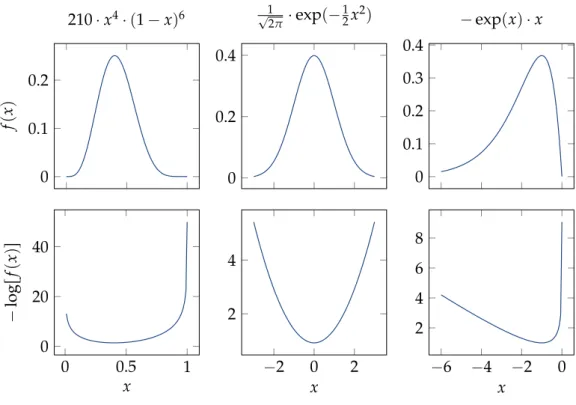
0 0.1 0.2 f p x q 210¨x4¨ p1´xq6 0 0.2 0.4 1 ? 2π¨expp´ 1 2x2q 0 0.1 0.2 0.3 0.4 ´exppxq ¨x 0 0.5 1 0 20 40 x ´ log r f p x qs ´2 0 2 2 4 x ´6 ´4 ´2 0 2 4 6 8 x
Figure 1.6:Three non-convexfunctions (top) withconvexnegative logarithms (bottom).
Proof. To show equivalence, we need to show that Equations 1.9, 1.10, and 1.11 hold. Equation1.9holds trivially becauseφis strictly monotonously increasing.
Regarding Equation1.10 note that strictly monotonously increasing functions are injective and thus invertible (if restricted to their image). Therefore, we obtain:
gip~xq ě0 ðñ ρi ` gip~xq ˘ ěρip0q ðñ ρi ` gip~xq ˘ ´ρip0q ě0
Using the same invertibility reasoning, we also know for all jthat
hjp~xq “0 ðñ ψj ` hjp~xq ˘ “ψjp0q ðñ ψj ` hjp~xq ˘ ´ψjp0q “0
Example 44(Log-convex functions). The following functions are not convex but become convex by applying a negative logarithm:
• binomial density functions: fpxq “ ˆ
n k ˙
xk¨ p1´xqn´k for x P r0, 1s, with the
negative logarithm ´logrfpxqs “ ´logr ˆ
n k ˙
s ´k¨logrxs ´ pn´kq ¨logr1´xs.
• Gaussian density functions: fpxq “ ?1
2πexpp´ 1
2x2q, with the negative logarithm ´logrfpxqs “ 12logr2πs `12x2.
• fpxq “ ´x¨exppxq with the negative logarithm´logrfpxqs “ ´logr´xs ´x. Also refer to Figure1.6.
1.4 D U A L I T Y
While differentiable optimization gives us a tool to solve unconstrained, continuous
optimization problems, we are still missing an equivalent tool forconstrainedoptimization problems. The main trick to address such problems is to re-write them as unconstrained problems or at least less severely constrained problems. We call such a re-written form of an optimization problem its dual form. In this section, we will cover two kinds of dual forms, namely the Lagrange and the Wolfe dual, and we will also establish the equivalence of primal and dual form under certain conditions.
1.4.1 Lagrange Dual Form
Definition 45(Lagrange dual). Let min
~xPRK fp~xq
s.t. gip~xq ě0 @iP t1, . . . ,mu hjp~xq “0 @jP t1, . . . ,nu
be anoptimization problemin standard form. Then, we define theLagrange dualof the problem as follows. sup ~λPRm,~µPRn inf ~xPRK fp~xq ´ m ÿ i“1 λi¨gip~xq ´ n ÿ j“1 µj¨hjp~xq (1.36) s.t. λi ě0 @iP t1, . . . ,mu
Whenever we consider a Lagrange dual, we call the original problem the primal
problem.
We call the function
L:RKˆRmˆRnÑR where Lp~x,~λ,~µq:“fp~xq ´ m ÿ i“1 λi¨gip~xq ´ n ÿ j“1 µj¨hjp~xq (1.37)
theLagrangianof the problem.
We call the variablesλi andµj theLagrange multipliersof theLagrange dual.
Remark 46(Infimum and supremum). We introduced supremum and infimum notation here, which is necessary for mathematical reasons. Broadly speaking, however, sup is the same as max and inf the same as min, just that sup and inf can also obtain infinity values.
Example 47(Lagrange dual). Consider the followingoptimization problem. min
x,yPR x´y
s.t. x2`y2“1
The Lagrange dualfor this problem is given as: sup
µPR
inf
x,yPR x´y´µ¨ px
Instead of solving the original problem, we can now solve this simpler version, which is unconstrained.
In a first step, we compute the gradient and Hessian: ∇x,yLpµ,x,yq “ ˆ 1´2µ¨x ´1´2µ¨y ˙ and ∇2 x,yLpµ,x,yq “ ˆ ´2µ 0 0 ´2µ ˙
By solving the equation∇x,yLpµ,x,yq “~0 for xandywe obtainx“ 2µ1 andy“ ´2µ1. By plugging this result in turn into our original side constraints x2`y2“1 we obtain
` 1 2µ ˘2 ``´ 1 2µ ˘2 “1 ðñ µ2“ 2 22 ðñ µ“ ˘ 1 ? 2 By inspecting the Hessian we see that only the solutionµ“ ´?1
2 yields alocal minimum.
Accordingly, we obtain the solutionx “ ´?1
2 andy“ 1 ?
2 with objective function value x´y“ ´?2.
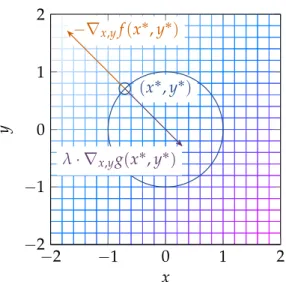
Remark 48(Interpretation as two-player game). The intuition behind theLagrange dual
can be phrased as a game of yourself against a malicious opponent. In this game, you want thatLp~x,~λ,~µqgets as small as possible and your opponent wants that it gets as big as possible. You have control over the variable~xand your opponent over the variables~λ
and~µ. If you violate any of the constraints, your opponent can punish you by setting the
corresponding Lagrange multipliers to large values such that you do not achieve the low optimization value you hoped for. Therefore, to achieve the least possible value, you are not allowed to violate the constraints and thus the primal and duel problem correspond to each other.
However, as we will see in the next section, the Lagrange dual and the original problem are notstrictlythe same, although the difference is subtle.
1.4.2 Duality Gaps
Remark 49 (Duality gaps in terms of the game metaphor). To understand the subtle difference between dual and primal, let’s return to the two-player game metaphor from Remark 48. We said that theLagrange dualcan be understood as a game where you control the variable ~x and wish to minimize the Lagrangian Lp~x,~λ,~µq whereas your opponent controls the vairables~λand~µand wants tomaximizethe LagrangianLp~x,~λ,~µq.
The subtle problem in this game is that theLagrange dualassumes thatyour opponent must move first, whereas you can then choose~x in perfect knowledge of your opponents choices. In this scenario, your opponent must try to forsee what you will choose and select their variables conservatively, thus potentially giving you more points than they’d like. In the primal problem, though,youmust choose first and your opponent can punish you for wrong variable choices.
The difference in the outcome values of both versions of the game is called theduality gap.
Definition 50(Duality gap, weak duality, strong duality). The difference f˚´L˚between
We say that weak duality holds for an optimization problem if the duality gap is non-negative.
We say thatstrong dualityholds for anoptimization problemif the duality gap is zero. Theorem 51 (Weak duality theorem). For everyoptimization problem, weak duality holds. Proof. We first prove a much more general result, namely the max-min inequality.
LetX,Y be two arbitrary sets and letLbe some functionL:X ˆY ÑR. Further,
letφbe the functionφ:X ÑRwithφpxq:“infyPYLpx,yq. Now, for anyxPX,Lpx,yq
must be at least as big asφpxq, otherwiseφpxqwould not be the infimum over ally. In
other words, we obtain:
Lpx,yq ěφpxq @xPX,yPY
Further, if we now maximize over x, supxPXLpx,yq is at least as large as supxPX φpxq. Otherwiseφpxqwould, again, not be the infimum. Formally, we obtain:
sup
xPX
Lpx,yq ěsup
xPX
φpxq yPY
Finally, because this inequality holds for allyPY, it also holds for the infimum, which yields the max-min inequality:
inf
yPY supxPX Lpx,yq ěsupxPX yinfPY Lpx,yq (1.38)
Next, let min ~xPRK fp~xq s.t. gip~xq ě0 @iP t1, . . . ,mu hjp~xq “0 @jP t1, . . . ,nu
be anoptimization problemin standard form. Then we can define the following problem: min ~xPRK φp~xq where φp~xq “ sup ~λPRm `,~µPRn Lp~x,~λ,~µq
and whereLis the Lagrangian of the original problem (refer to Equation 1.37).
This problem is equivalent because for any~xthat is not in thefeasible set,φp~xqobtains the value8, and for any~xin thefeasible set,φp~xq “ fp~xq. Therefore, the duality gap is exactly the difference between the optimalobjective functionvalues for our equivalent problem and the solution of the Lagrange dual. The optimal value of the equivalent problem is per definition above:
inf ~xPRK sup ~λPRm `,~µPRn Lp~x,~λ,~µq
whereas the optimal value of theLagrange dualis per definition: sup ~λPRm `,~µPRn inf ~xPRK Lp~x, ~λ,~µq
Example 52(Strong duality counterexamples). There exist optimization problems, even
convexones, where strong duality doesnothold. First, consider a simple non-convexexample.
min
x,yPR,yą0 x 2
s.t. x¨y´yě0
Note that this is equivalent to minimizingx2such thatxě1. The solution to this problem is thus obviously x“1 with fp1q “12 “1. Now, consider theLagrange dual.
sup λPR inf x,yPR,yą0 x 2´ λ¨ px¨y´yq s.t. λě0
Because the inner optimization problem receives λ as input, we can set y “ e λ for
arbitrarilyeą0, resulting in the LagrangianLpx,e
λ,λq “x
2´e¨ px´1q. This Lagrangian
has the derivative B
BxLpx,λe,λq “ 2x´e and the second derivative B2 B2xLpx,
e
λ,λq “ 2.
Therefore, we obtain a minimum forx“ e
2. Because we can seteto arbitrarily small values
larger than zero, we obtain an infimum of zero. Note that this infimum is independent of λ, such that our overall solution is 0 as well. Therefore, we obtain a duality gap of
1´0“1ą0.
Our next example is due toTan (2015). Consider the problem min
x,yPR,yą0 expp´xq
s.t. ´x 2 y ě0,
which isconvex. Note that the only possible feasible value forxis 0 because otherwise theinequality constraint would be violated. Therefore, the minimalobjective function
value is 1.
Now, consider theLagrange dualof this problem: sup λPR inf x,yPR,yą0 expp´xq `λ¨ x2 y s.t. λě0
Because the inner minimization problem has access to the value of λ, we can simply
set y“x3¨λand thus obtain the alternativeobjective functionexpp´xq `1x, which is is minimized by setting xto arbitrarily large values, thus achieving an infimum of zero. Note that this infimum is independent ofλ, such that our overall solution is zero as well,
yielding a duality gap of 1´0“1ą0.
The last example begs the question when strong dualityisguaranteed. As it turns out, it is hard to characterize necessary conditions for strong duality. But we do now
sufficientconditions, the broadest of which isSlater’s condition. Definition 53 (Slater’s condition). Let
min ~xPRK
fp~xq