Distributed variance regularized Multitask Learning

Distributed Variance Regularized Multitask Learning

Michele Donini

, David Martinez-Rego

, Martin Goodson

, John Shawe-Taylor

, Massimiliano Pontil

†_{University College London, Malet Place, London WC1E 6BT, UK} ‡_{Skimlinks, London, UK}

§_{Istituto Italiano di Tecnologia, Via Morego, Genoa, Italy}

Abstract—Past research on Multitask Learning (MTL) has focused mainly on devising adequate regularizers and less on their scalability. In this paper, we present a method to scale up MTL methods which penalize the variance of the task weight vectors. The method builds upon the alternating direction method of multipliers to decouple the variance regularizer. It can be efficiently implemented by a distributed algorithm, in which the tasks are first independently solved and subsequently corrected to pool information from other tasks. We show that the method works well in practice and convergences in few distributed iterations. Furthermore, we empirically observe that the number of iterations is nearly independent of the number of tasks, yielding a computational gain ofO(T)over standard solvers. We also present experiments on a large URL classification dataset, which is challenging both in terms of volume of data points and dimensionality. Our results confirm that MTL can obtain superior performance over either learning a common model or independent task learning.

I. INTRODUCTION

Multitask Learning (MTL) is nowadays an established area of machine learning that has shown its benefits in many applications. MTL aims at simultaneously learning models for multiple related tasks by inducing some knowledge transfer between them. A typical MTL algorithm introduces a regularization term or prior that imposes an adequate shared bias between the learning tasks. This idea was inspired by research on transfer learning in psychology, which brought up the hypothesis that the abilities acquired while learning one task (e.g. to walk, to recognize cars, etc.) presumably apply when learning a similar task (to run, to recognize trucks, etc.) [Silver and Mercer, 1996], [Thrun, 1997] and was first coined inside the machine learning community in the 90’s [Caruana, 1997], [Thrun, 1997]. The notion of what “task relatedness” means in practice is still not completely clear but theoretical studies support the intuition that training simultaneously from different related tasks is advantageous when compared to single task learning [Baxter et al., 2000] [Ben-David et al., 2003] [Maurer et al., 2006]. The benefits usually include more efficient use of small data sets in new related tasks and improved generalization bounds when learning simultaneously.

Recent successful studies on large datasets suggest that the use of models whose training process can be scaled up in terms of the size of the database is key to obtain good results. In large scale learning scenarios, the reduction of the estimation error that can be achieved by leveraging bigger datasets compensates the bias introduced by the use of simpler models

such as linear classifiers [Bottou et al., 2008]. This trend has produced several algorithms that put the focus on scaling up the training of simple linear models such as support vector machines to PB of data, see [Shalev-Shwartz et al., 2014] and references therein. Despite this success, the MTL community has targeted the formulation of different regularizers that foster the correct information sharing between tasks in specific situations, overlooking their scalability. Nevertheless, MTL formulations apply very naturally to many large scale scenarios where we expect heterogeneous (although related) regimes to be present in the data.

Scalability of MTL can be challenged from two different angles. Recent applied studies on MTL [Birlutiu et al., 2013] [D’Avanzo et al. 2013] [Bai et al., 2012] [Huang et al., 2013], tackle scenarios such as preference learning, ranking, advertising targeting and content classification. Those studies mainly focus on the scalability when the number of examples increases. But scalability issues can also be encountered when the number of tasks grows. Think for example about learning: i) the preferences of a client on a per client basis, ii) the categorization of webpages on a per host basis or iii) the relevance of a query-document pair for a specific combination of user aspects like region, sex, age, etc. A common feature of these applications is that: (a) many tasks suffer a lack of data to learn from, and (b) the number of free parameters to learn grows with the number of tasks. The first issue has been one of the main motivations of multitask learning, namely to leverage data from similar tasks in order to improve accuracy. On the other hand, the second challenge could impose a limitation on the learning process if the number of tasks grows big since it means a larger amount of data to transfer on the network, stored and managed by the learning algorithms. Thus, if we combine MTL with parallel optimization, we would obtain a practical process that is expected to obtain higher accuracy.

A. Our Contribution

A key goal of this paper is to equip one of the most widespread MTL methods presented in [Evgeniou and Pontil, 2004] with a parallel optimization procedure. For this purpose, we employ the alternating direction method of multipliers (ADMM), see for example [Eckstein and Bertsekas, 1992], [Boyd, 2010] and references therein. We focus on MTL methods which involve the variance

of the task weight vectors as the regularizer. We show that the optimization process can be efficiently implemented in a distributed setting, in that the different tasks can first be independently solved in parallel and subsequently corrected to pool information from other tasks. We report on numerical experiments, which indicate that the method works well and converges in few distributed iterations. We empirically observe that the number of iterations is nearly independent of the number of tasks, yielding a computational gain of O(T)over standard solvers. We also present experiments on a large URL classification dataset, which is challenging both in terms of volume of data points, dimensionality and number of different tasks. Our results confirm that MTL can obtain superior performance over either learning a common model or independent task learning.

B. Related Work

The study of parallel MTL systems has been introduced in some previous works. In [Dinuzzo et al., 2011] the authors present a client-server MTL algorithm which maintains the privacy of the data between peers. Their method applies to the square loss function. In this paper we focus on the hinge loss, however our algorithm readily applies to other convex loss functions. It also preserves the privacy of data from different tasks since this does not need to leave client’s side. In [Ahmed et al., 2014], the authors develop a parallel MTL strategy for hierarchies of tasks. This solution is based on Bayesian principles and presents some limitations when implemented on a MapReduce platform. In comparison, our approach takes a maximum margin approach that, although it does not include any hierarchy of tasks, maps naturally to any MapReduce environment and establishes the underpinnings to be extended to more complex situations. Very recently, in [Wang et al., 2015], the authors presented a distributed algorithm for group lasso multitask learning, addressing its statistical properties.

The paper is organized as follows. In Section 2 we briefly review the notation and the MTL method. We present our approach for making the optimization separable in Section 3. In Section 4, we describe in detail the main steps of the proposed algorithm. In Section 5 we present a stochastic gradient descent method to solve the inner SVM optimization problem and detail the convergence properties of this process. Experimental results with both artificial and real data are detailed in Section 6. Finally, In Section 7 we draw our conclusions and discuss perspectives for future work.

II. BACKGROUND

When we refer to multitask learning (MTL) we mean the following situation. We haveT learning tasks and we assume that all data from these tasks lie in the same space Rd×Y, where Y ={−1,1} for binary classification andY =R for regression. Associated with each tasktwe havemtdata points

(x1t, y1t),(x2t, y2t), . . . ,(xmtt, ymtt) (1)

sampled from a distributionPt on X×Y . We assume that this distributionPtis different for each task but that different Ptare related. The goal is to learnT functionsh1, h2, . . . , hT

such that the average error _T1 T

P

i=1

E(x,y)∼Pt[`(y, ht(x))]is low for a prescribed loss function `. Note that when T = 1, this framework includes the single task learning problem as a specific case.

In [Evgeniou and Pontil, 2004] an intuitive formulation for relatedness between tasks inspired by a hierarchical bayesian perspective was presented. This formulation assumes that the hypothesis class of each individual task is formed by the set of linear predictors (classifiers) whose parameter vectors are related by the equations

wt=vt+w0, t= 1, . . . . , T. (2)

The vector vt models the bias for task t and the vector

w0 represents a common (mean) classifier between the tasks.

Within this setting, the tasks are related when they are similar to each other, in the sense that the vectorsvthave small norms compared to the norm of the common vector w0. Note also

that this setting may be useful in a transfer learning setting, in which we do not have data for a new task but we can still make predictions using the common averagew0.

In the above setup, an optimalw0 and a set of optimalvt for each task is found by solving the following optimization problem which is an extension of linear SVMs for a single task (which corresponds to the caseT = 1), namely

min w0,vt ( _T X t=1 ft(w0+vt) + λ1 T T X t=1 kvtk22+λ2kw0k22 ) (3) whereft(·) =Pmt

i=1`(yit,h·,xiti), the empirical error for the

taskt.

Define the variance of the vectorsw1, . . . ,wT as

Var(w1, . . . ,wT) = 1 T T X t=1 wt− 1 T T X s=1 ws 2 2 . It can be shown [Evgeniou and Pontil, 2004, Lemma 2.2] that problem (3) is equivalent to the problem

min wt ( T X t=1 ft(wt) +ρ1kwtk22 +ρ2T Var(w1, . . . ,wT) ) (4) where the hyperparameters are linked by the equations

ρ1= 1 T λ1λ2 λ1+λ2 , ρ2= 1 T λ2 1 λ1+λ2 .

This connection makes it apparent that the regularization term encourages a small magnitude of the vectorswt(large margin of each SVM) while simultaneously controlling their variance.

III. DISTRIBUTEDMTLVIAADMM

The utility of problem (4) is that its objective function – unlike that in problem (3) – is almost separable across the different tasks. Namely, the only term in the objective function in (4) that prevents decoupling is the last summand,

which makes the gradients for different tasks dependent. If we could remove this dependency, both the data and weight vectors for different tasks could be maintained in different nodes of a computer cluster without the need of centralizing any information and so making the method scalable. For this purpose we use an optimization strategy based on the alternat-ing direction method of multipliers (ADMM), see for example [Boyd, 2010], [Eckstein and Bertsekas, 1992] and references therein. This method solve the general convex optimization problem

minimize

w,z f(w) +g(z)

subject to Mw=z

(5) where f and g are two convex functions. Different al-gorithms have been proposed to tackle this optimiza-tion with different convergence characteristics, see, for ex-ample, [Boyd, 2010], [Mota et al., 2011], [He et al, 2012], [Hong, 2013]. In this paper we employ the ADMM algorithm outlined in [Eckstein and Bertsekas, 1992]. Although poten-tially faster algorithms exists, such as [Goldstein et al., 2014], their convergence analysis require stronger assumptions which are not meet in our problem.

We define the augmented Langrangian function Lη at

w,z,y as Lη(w,z,y) =f(w) +g(z) +hy, Mw−zi +η 2kMw+zk 2 2

where η is a positive parameter. Each ADMM step requires the following computations

wk= argmin x Lη(w,zk−1,yk−1) zk= argmin z Lη(wk,z,yk−1) yk= yk−1+η(Mwk−zk) (6)

where k is a positive integer and z0, y0 are some starting points. We call each round of (6) an ADMM iteration. This process is repeated until convergence.

A convenient identification between problem (4) and the ADMM objective function (5) shows that the multitask objec-tive can be efficiently optimized through this strategy. Namely, problem (4) is of the form (5) for the choice M =I and

f(w) = T X t=1 ft(wt) + ρ1 2 T X t=1 kwtk22 g(z) =ρ2T Var(z1, . . . ,zT) + ρ1 2 kzk 2 2

where we setw to be the concatenation of the weight vectors

wt for all the tasks, and we force z= w in order to make f(w) +g(z) equal to the original objective in the feasible region.

The augmented Lagrangian for this specific case is Lη(w,z,y) = T X t=1 ft(wt) + ρ1 2 T X t=1 (kwtk22+kztk22) +ρ2T Var(z1, . . . ,zT) +hy,w−zi+ η 2kw−zk 2 2.

Using this expression, the first three updating equations in the ADMM optimization strategy (6) become

wk = argmin w T X t=1 ft(wt) + T X t=1 ρ1 2 kwtk 2 2 +hykt−1,wti+ η 2kwt−z k−1 t k 2 2 zk = argmin z ρ2T Var(z1, . . . ,zT) + ρ1 2 kzk 2 2 − hyk−1_,zi+η 2kw k−1_−zk2 2 yk =yk−1+η(wk−zk). (7)

We are left to analyze how to solve the first two optimization steps to obtain wk and zk. It is noticeable that in the first of these steps the optimization over the tasks is completely decoupled, that is the component vectorswk

t can be computed independently of each other – we discuss how to do this in Section V. Thus, the update of each task’s weight vector can be run in parallel with no communication involved once data is distributed by tasks. As we shall see in Section IV-B the second optimization step, in which the only information sharing between the tasks occurs, can also be carried out with minimal communication just by averaging the vectors for the different tasks, hence leading to an scalable strategy.

IV. ALGORITHM

In the previous section we showed how the MTL problem in equation (3) or (4) can be solved by the iterative scheme (6). In this section, we analyse the minimization problems for

wk _andzk_{, noting that both can be computed in a distributed} fashion.

A. Optimization of each individual task

The update formula for the weights w in (7) can be implemented with different methods. The optimization of the weights completely decouple across the taskswtand each can be compute by solving the problem

min wt ft(wt) + ρ1+η 2 kwtk 2 2+hyt−ηzt,wti . (8) One natural approach is to use (sub)gradient descent, possibly in a stochastic setting when the number of datapoints of a task is large. In this paper we consider the case that`is the hinge loss, namely `(y, y0) =h(yy0), where h(·) = max(0,1− ·). In Section V we detail a stochastic gradient descent method to solve problem.

B. Optimization of the auxiliary variables

The update step for the auxiliary variable zk _{is more} advantageous computationally since we can work out a closed formula. The objective function is given by

ρ2 T X t=1 zt− 1 T T X s=1 zs 2 2 +ρ1 2 kzk 2 2+hy k_,wk_−zi+η 2kw k_−zk2 2

for fixed wk _{and y}k_{. Removing constant terms that do not} depend on z, this can further be rewritten as

F(z) = z, ρ2DTD+ ρ1 2 I z −hyk_,zi+η 2 kzk 2 2−2hw k_,zi

where matrixD∈RT d×T dis given in block form as

D=          DM D0 D0 · · · D0 D0 DM D0 · · · D0 D0 D0 DM · · · D0 .. . ... ... ... ... D0 D0 D0 · · · DM          , (9)

beingdthe number dimensions of a block andT the number of blocks. Finally, DM = T_T−1Id×d andD0 =−_T1Id×d, where

Id×d is thed×didentity matrix.

If we take the derivative of the above objective function we can see that the optimal solution can be found by solving the system of linear equations

(2ρ2DTD+ (ρ1+η)I)zk= (yk+ηwk).

The following lemma shows that the inverse E = (2ρ2DTD+ (ρ1+η)I)−1 has a convenient closed analytical

formula.

Lemma 1. LetE= (2ρ2DTD+ (ρ1+η)I)−1, where matrix

D ∈RT d×T d is defined equation (9). The matrix E has the following structure E=         EM E0 E0 · · · E0 E0 EM E0 · · · E0 E0 E0 EM · · · E0 · · · · E0 E0 E0 · · · EM         ∈_RT d×T d

where EM and E0 are:

EM = 1 T ₁ η+ρ2 + T −1 η+ 2ρ1+ρ2 Id×d, E0= 2ρ1 T(η+ρ2)(η+ 2ρ1+ρ2) Id×d.

Proof. We have to prove that (2ρ2DTD + (ρ1 +η)I)E =

E(2ρ2DTD+(ρ1+η)I) =I∈RT d×T d. The first observation of the proof is the particular structure of the matrix D that is an idempotent symmetric matrix and then DT_{D =D}2_=D.

So, the matrix 2ρ2DTD+ (ρ1+η)I is also equal to G = 2ρ2D+ (ρ1+η)I and has the following structure inRT d×T d

     GM G0 · · · G0 G0 GM · · · G0 · · · · G0 G0 · · · GM      (10) where G0 = 2ρ2D0,GM = 2ρ2DM + (ρ1+η)Id×d, where

Id×d is the identity matrix in d dimensions. Then, we can

evaluate the block product between E and G. This product generates a block matrix where each block on the diagonal is

(T−1)E02ρ2D0+EM(2ρ2DM+ (ρ1+η)Id×d) =Id×d,

and the off-diagonal block are zero, since

(T−2)E02ρ2D0+E0(2ρ2DM + (ρ1+η)Id×d)

+EM2ρ2D0= 0d.

This formula reveals that the optimization over z1, . . . ,zT can also be run in parallel. First, we can reduce the vectors from all the tasks to a single vector w = E0

T

P

t=1

wt. Then, each vector can be updated in parallel by using againEM and E0. Similarly to the optimization of wt, this operation can

be readily done in a framework such as MapReduce to speed up computations with a very reduced need of broadcasting information.

C. Convergence

We comment on the convergence properties of our method. Our observations are a direct consequence of the gen-eral analysis in [Eckstein and Bertsekas, 1992]. Specifically, [Eckstein and Bertsekas, 1992, Theorem 8] applies to our problem, with (using their notation) ρk = 1for every k∈N, their pequal to our y and theirλequal ourη. The theorem requires that the matrix M is full rank, f and g are closed proper convex functions and the sum of the errors of the inner optimization problems is finite. All these hypothesis are meet in our case. In particular, the optimization overzis performed exactly as discussed in Section IV-B. The optimization over

w are the parallel SVMs which we can solve to arbitrary precision using for example gradient descent. As we will see in our numerical experiments only few iterations are sufficient to reach a good suboptimal solution and gradient descent may be replaced by its stochastic version (discussed below) without affecting the good convergence of the algorithm.

V. SGD OPTIMIZATION OF EACH INDIVIDUAL TASK

When we have to solve problems with a large number of points, it is not computationally feasible to solve the optimization of each individual task with batch algorithms. In this section, we observe that it is possible to exploit a Stochastic Gradient Descent (SGD) strategy for our proposed method. Firstly, we show that the optimal solution of the optimization problem is contained inside a convex ball. From this results, we are able to satisfy the hypothesis of conver-gence of the SGD technique for strongly convex functions [Rakhlin et al., 2012], [Shalev-Shwartz et al., 2014]. Specifi-cally, we prove the boundedness of the directions followed in the SGD optimization of w, in each outer step k≥0 of the ADMM strategy.

Algorithm 1 depicts the optimization of the weight vectors

wt using the SGD for strongly convex functions. The opti-mization for each task presented in Equation 8 is equivalent to the problem minwtFt(wt), where

Ft(wt) =Lt(wt) + γt 2kwtk 2 2, Lt(wt) = 1 mt mt X i=1 h(yithwt,xiti) +hyt−ηzt,wti !

and γt = (ρ1+η)/mt. In order to be able to apply SGD

we need to sample a direction ut at each step q such that E[ut|wt] is a subgradient of Ft at wt. If at each step we sample randomly and with replacement a pattern xit from the training set, the following sequence of directions complies with the above restriction

ut=

(

γtwt+_m1(yt−ηzt) if yithwt,xiti ≥1,

−yitxit+γtwt+m1(yt−ηzt) otherwise.

In the following lemma, we show that the optimal solution of the original optimization problem resides inside a convex ball.

Lemma 2. Ifw∗ is the optimal solution of problem (4) then

kw∗_k 2≤ q T M 2λ1, whereM = T P t=1 mt. Proof. Let µ= T λ2

λ1 . We make the change of variables w=

√

µw0,v1, . . . ,vT ∈ R(T+1)d and introduce the map φ : Rd× {1, . . . , T} 7→R(T+1)d, defined as φ(x, t) = _x √ µ,0, . . . ,0,x,0, . . . ,0 . (11) Following [Evgeniou and Pontil, 2004] we rewrite problem (3) as a standard SVM problem in the extended input space for the feature map (11), namely

min w ( C M X i=1 h(yihw, φ(xi, ti)i) +1 2kwk 2 2 ) where C = T 2λ1 and M = T P t=1

mt. Since at the optimum the gap between the primal and dual objective vanishes, there existsα∗∈[0, C]M _{such that}

1 2kw ∗_k2 2+C M X i=1 h(yihw, φ(xi, ti)i) = M X i=1 α∗_i −1 2kw ∗_k2 2.

Using the fact that M P i=1 h(yihw, φ(xi, ti)i) ≥ 0 we conclude that kw∗_k2 2≤ PM i=1α ∗ i ≤M C= T M 2λ1 =β.

This lemma thus proves that in Algorithm 1 it is safe to restrict the set of feasible solutions to the ball B := {x ∈ Rd : kxk22 ≤ β} with

β = max(pT M/(2λ1),

p

M/(2λ1)) and it justifies

the projection step at line 7 of the algorithm.

Algorithm 1 Optimization of each individual task

Input: Dataset{(xit, yit), i= 1, . . . , mt}for task t, parame-tersρ1,γt,η,zt,yt,T,M

Output: Optimal weight vectorwt

1: w0t ←0

2: γt ← ρ1m+tη

3: forq←1ton do

4: δ← 1

qγt

5: Choose a random pattern(xit, yit)from the set

6: wq+ 1 2 t ←w q t−δut 7: wq_t+1 ← min 1, β 1 kwq+ 12 t k2 wq+12 t 8: return wˆt= _n2 n P q=n 2+1 wq_t

Now, we analyze the convergence of Algorithm 1 and we base our proof on a recent result presented in [Rakhlin et al., 2012], [Shalev-Shwartz et al., 2014] which states (adapting their result to our notation) that the aforemen-tioned strategy converges with the rateE[Ft( ˆwt)]−Ft(wt)≤

ρ2

2γtn after n iterations, provided when Ft(w) is γt-strongly convex andE[kutk2]≤ρ2for some finite constantρ. Clearly, the objective function Ft is strongly convex with constant γt = ρ1+η

mt , see [Shalev-Shwartz et al., 2014, Lemma 13.5]. We are left to prove that the directionsutfollowed in the SGD optimization of w in each outer step k ≥ 0 of the ADMM strategy are bounded, which we state in the following theorem.

Theorem 1. If all the examplesxitsatisfykxitk22≤Rthen for

every iterationk ∈_N of the outer ADMM scheme and every inner iterationq, there existsρ >0such that the directions of the SGD in Algorithm 1 are bounded in average,_E[kuk

tk22]≤

ρ2_{<+∞for everyt= 1, . . . , T.}

Proof. At each outer stepk, the direction for the taskt is:

uk_t = ( γtwkt +m1(y k t −ηzkt) if`kit= 0, −yitxit+γtwtk+ 1 m(y k t −ηzkt) if`kit>0 where we use the shorthand`k

it=yithwt,xiti.

We are interested in finding a bound for the quantitykuk tk22.

From the definition we have that

kuk tk 2 2≤ kyitxitk22+γ 2 tkw k tk 2 2+ 1 m2(ky k tk 2 2+η 2_kzk tk 2 2).

We have already shown that kwk

tk22 ≤ β and from the

hypothesis we have thatkyitxitk22≤R. Now, we are interested

in finding a finite bound for the quantity kyk

tk22+η2kzktk22.

From the initialization of the algorithm, we have thatky1

tk22+

η2_kz1

tk22<+∞. In fact,ky1tk22<+∞andkz1tk22<+∞. We

can use the induction for the valuekyk tk 2 2+η 2_kzk tk 2 2changing

the stepk. We can exploit the hypothesis that

kyi tk 2 2+η 2_kzi tk 2 2<+∞, ∀i < k and thenkyi tk22<+∞andη2kzitk22<+∞, ∀i < k.

By definition, the following inequalities hold kyktk 2 2≤ ky k−1 t k 2 2+kηw k−1 t k 2 2+kηz k−1 t k 2 2 ≤ kyk−1 t k 2 2+η 2_β+η2_kzk−1 t k 2 2 ≤ ky1 tk 2 2+ k−1 X i=2 η2(β+kzi tk 2 2) =: Φ k t.

By the induction hypothesis the value Φk

t <+∞. Also, we have that kzk tk 2 2≤ kEk 2 2(ky k tk 2 2+η 2_kwk tk 2 2),

whereE= (2ρ2DTD+ (ρ1+η)I)−1 is symmetric and then

kEk2

2 is its spectral radiusrE∈R+. Then, we can claim that

kzktk 2 2≤rE(kyktk 2 2+η 2_β) ≤rE(Φkt+η 2_{β) =: Ψ}k t <+∞. Finally, the following bound holds:

kuk tk 2 2≤R+γ 2 tβ+ 1 m2(Φ k t +η 2_Ψk t) :=ρ 2_<+∞.

VI. EXPERIMENTAL RESULTS

In this section present numerical experiments which high-light the computational efficiency of our algorithm, and report on the advantage offered by the MTL strategy in formula (3) in a challenging url classification dataset. Our implementation is available at https://github.com/torito1984/MTLADMM. A. Artificial data

In the first experiment we generated an artificial dataset which is captured by the model (2) and, in addition, introduces a set of irrelevant features.

The number of relevant and irrelevant features was set to

8 and100, respectively. The dataset is made of400 different binary classification tasks,5of which have 1000patterns and the rest 16 patterns. To generate the data we first sample the components w01, . . . , w0d of the mean vector w0 iid form

a zero mean Gaussian with variance σ = 0.25. Then, we randomly pick 5 of the relevant features and create a vector

wtfor each task by adding a Gaussian perturbation with zero mean and standard deviation σi = 2w0i. Next for each task,

we generate a balanced set of points on each side of the classification hyperplane. To generate a point we: (1) pick a sign swith a50% chance, (2) starting from the origin, move in a random directionsdwheredis the normal vector of the classification hyperplane and p∈ N(5,0.1) (this generates a well behaved dataset with some random margin violations), (3) finally we choose a random direction in the subspace of dimension d−1 parallel to the classification hyperplane and make a jump with magnitude sampled from N(0,20). Since we are generating patterns with a low margin covering many different directions in the parallel subspace, only the tasks with

1000patterns have enough data to achieve high test accuracy by their own. For the rest of the tasks – which account for around 55% of the dataset – the number of points is insufficient to achieve a reasonable solution and they should benefit from

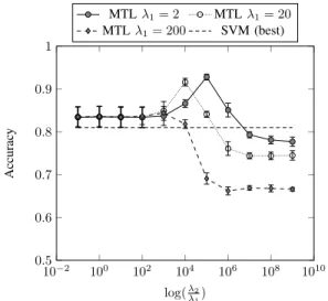
10−2 ₁₀0 ₁₀2 ₁₀4 ₁₀6 ₁₀8 ₁₀10 0.5 0.6 0.7 0.8 0.9 1 log(λ2 λ1) Accurac y MTLλ1= 2 MTLλ1= 20 MTLλ1= 200 SVM (best)

Fig. 1. Classification performance for the artificial classification dataset

an MTL approach. We will see that a similar situation arises in the real dataset we cover hereunder.

Returning to formula (3), it is instructive to observe that, for a fixed λ1 > 0, if we let λ2 → ∞, the optimization

problem is equivalent to training separate linear SVMs on each task. In this situation and in high dimension, the method will overfit the dataset. On the other hand, for a fixedλ2 >0, if

we let λ1 → ∞, the optimization problem is equivalent to

training a single linear SVMs on the full dataset, which may underfit the data. In practical situations, we expect the optimal hyperparameters to lay in between these two situations, and obtaining lower accuracy for both extremes.

1) Classification performance: Figure 1 depicts the average test accuracy for a 10-fold CV in the aforementioned dataset. Solid lines depict the accuracy of the proposed algorithm for different values of λ1 and λ2. As expected, the optimal

hyperparameters lay in between both extremes forλ2/λ1 and

overfitting arises for when λ2 λ1. The dotted line depicts

the accuracy of a single SVM trained with a state of the art op-timization algorithms for linear SVMs in [Hsieh et al., 2008]. We can observe that, with appropriate hyperparameters, MTL is superior to single task learning thanks to the information sharing.

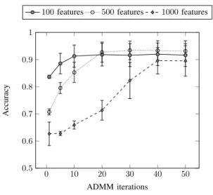
2) Convergence: One question that may arise is how many ADMM iterations are needed to achieve a good result in practice. This would be the major bottleneck of the proposed method since ADMM iterations are sequential. We ran exper-iments with the same data generation strategy and varying the dimensionality. The number of relevant features was kept at 10% of the dimensionality.

First, in Figure 2, it can be observed that a higher dimension slows down the convergence to the optimum in the first itera-tions, an order of tens of iterations is enough to obtain a good accuracy. Second, we compared a MatLab implementation of the standard MTL called MALSAR1 in performance and

computational complexity varying the number of different tasks in the set {20,40,60,80,100,200,400,800,1200}. We keep the sample sizes per task fixed and measure MALSAR running time. For our method, we are interested in finding the number of outer ADMM iterations needed to converge to the same accuracy of MALSAR with a tolerance of 10−4.

In Table I, a comparison of the computational complexities is presented. We collected the CPU time required by the standard MTL implementation in order to find the optimal solution, varying the number of tasks. We compared these values with respect to the number of outer ADMM steps that our algorithm required to reach the same solution. For this purpose, we introduce the variable α= λ2

λ1+λ2. This variable

imposes the quantity of shared information among the tasks. In fact, whenαis equal to zero, we are training a single SVM for all the tasks, on the other hand, withα= 1we are training a different SVM for each single task.

In comparison we observed that the CPU time of MALSAR varies quadratically with number of tasks. For example for α= 0.5the CPU was of 3.3, 4.8,..., secs. for T=20,40,...,1200 From these results, we are able to claim that the standard MTL implementation has a quadratic complexity with respect to the number of tasks, whereas our ADMM implementation is able to reach the same optimal solution in a fixed number of outer steps. 0 10 20 30 40 50 0.5 0.6 0.7 0.8 0.9 1 ADMM iterations Accurac y

100features 500features 1000features

Fig. 2. Performance of ADMM with different dimensionality

B. URL classification

The next dataset was extracted from a production environ-ment in an online advertising firm. For online targeting, a data provider supplies data to an advertiser indicating which users are interested in specific product classes. In order to determine the interest of each user, web pages are first classified into interest categories (eg ‘fashion’, ‘photography’ etc). Thereafter the browsing behavior of users can be used to predict their interests. One way of achieving it is to predict the category of a page from the contents of a url. We can tackle this task using a bag-of-words strategy [Joachims, 2002]. Modern

Tasks MALSAR time (s) ADMM steps

α= 0.5 α= 0.0 α= 0.1 α= 0.5 α= 1.0 20 3.3 21 16 10 10 40 4.8 21 16 11 11 60 6.4 21 16 10 10 80 8.3 21 16 10 10 100 10.7 21 16 10 10 200 33.1 21 16 11 11 400 95.8 21 16 11 11 800 342.5 21 16 11 11 1200 698.3 21 16 10 10 TABLE I

CPUTIME OFMALSARALGORITHM AND NUMBER OF OUTER STEPS OF OURADMMALGORITHM IN ORDER TO REACH THE SAME ACCURACY OF MALSAR,WITH DIFFERENT AMOUNTS OF TASKS. THE VARIABLEαIS

EQUAL TOα= λ2 λ1+λ2

urls carry enough information to identify the page contents thanks to Search Engine Optimization strategies. Before being able to apply this, words should be detected and segmented into meaningful n-grams. This process can be easily achieved though a Viterbi-like strategy. The details of the algorithm used can be found in [Segaran et al., 2009, Ch. 4]. It calculates the most likely segmentation of a string containing text with no spaces based on a Viterbi-like probability maximization process and the prior probabilities of different n-grams ex-tracted from the 1 Trillion words dataset gathered by Google [Brants et al., 2006]. Once the URL is segmented, a bag-of-words representation is built.

The dataset treated is a collection of urls extracted from

Fig. 3. # of patterns per task (client) in the URL classification dataset.

the client base at Skimlinks labeled by humans as related to fashion or not. The dataset is a compound of over 500,000 urls extracted from 4,326 different client hosts embedded in a 150,000 dimension bag of words vector space. Thus, we have a binary classification task for a set of different tasks (clients/hosts). We hypothesize that different clients may use different vocabularies and ways of building urls, but that the underlying set of n-grams that indicate fashion should be shared between all of them. In addition, we can see in Figure 3 that the number of urls extracted from each client is highly skewed, so most tasks do not have enough data to

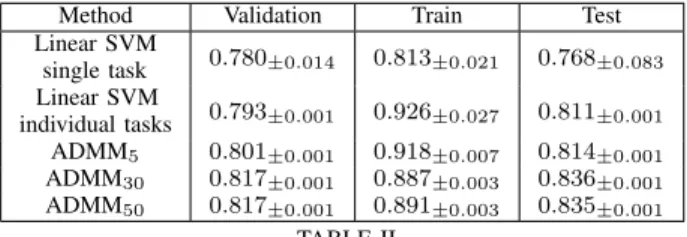
Method Validation Train Test Linear SVM single task 0.780±0.014 0.813±0.021 0.768±0.083 Linear SVM individual tasks 0.793±0.001 0.926±0.027 0.811±0.001 ADMM5 0.801±0.001 0.918±0.007 0.814±0.001 ADMM30 0.817±0.001 0.887±0.003 0.836±0.001 ADMM50 0.817±0.001 0.891±0.003 0.835±0.001 TABLE II

CLASSIFICATIONACCURACY±stdFORSKIMLINKS DATASET.

build a reliable model in such a high dimensional space. This problem’s scenario is similar to the artificial case previously treated and so we expect that sharing information between tasks could be beneficial.

Table II summarizes the results for the categorization dataset when compared to its single task and individual tasks coun-terparts. As it can be observed in the third column, there is an expected gain of 6% accuracy when compared with a single SVM model trained for all the the tasks and of 3% when compared to an SVM trained individually for each task. When comparing these results with the distribution of patterns per task, we can observe that there is enough variety between tasks that hinders SVM capacity to adapt to all of them. On the other hand, for less populated tasks there is not enough data to achieve a high accuracy and so all the information is not exploited. The capacity to transfer information embedded in MTL seems to balance the right amount of regularization and information sharing, giving the best results.

One of the questions in systems where an individualised response is needed is what to do in a cold start situation, i.e. what response to provide when we do not have data for some individual task. Single model training would advocate to use the same model as for all the tasks, whereas if we choose to have individualised models, we would lack the model for that case. It seems natural to think that the average model

w0 in formula (2), which constitutes the bias for any task

in the context, would be the right answer. In the previous dataset we discarded 29753 patterns from unpopulated task. So these tasks would be a sample of “cold start” of tasks we do not have data on. The accuracy of w0 and of the single

task SVM previously obtained are 82% and 80% respectively. When unified with the results in Table II, we can see that MTL shows a good adaptation to individual tasks and, at the same time, a good prior bias is also discovered.

VII. CONCLUSIONS ANDFUTUREWORK

In this work, we presented an algorithm for distributed MTL with task variance regularization. The iterations of the proposed algorithm are completely parallel and an accurate solution can be obtained in tens of iterations. The approach decouples the training of the different tasks by making use of an ADMM optimization scheme. We have tested the approach both on an artificial and on a real large scale datasets and proven that this MTL method can scale up to real large scale problems with better accuracy. We hope that our results will encourage further research on scaling up other MTL

methods and their application to real heterogeneous databases. The method presented could be readily extended to more general MTL regularizers of the form PT

s,t=1hws,wtiGst. An interesting question is for which classes of positive def-inite matrices G distributed optimization over the auxiliary variablesztwould still be possible, like in the case studied in this paper. For example, this should be possible when matrixG is the graph Laplacian of a tree as in [Khosla et al., 2012]. Yet another extension of the method presented in this paper arises in the context of multitask latent subcategory models as in [Stamos et al., 2015], where our algorithm could be employed to solve large scale image classification and detection problems for computer vision. Finally, ideas from [Suzuki, 2013] may be employed to obtain fully stochastic versions of our method. Acknowledgements: David Martinez Rego was supported by the Xunta de Galicia through the postdoctoral research grant POS-A/2013/196. We wish to thank Patrick Combettes, Taiji Suzuki and Yiming Ying for valuable comments.

REFERENCES

[Ahmed et al., 2014] A. Ahmed, A. Das, A.J. Smola. Scalable hierarchical Multitask Learning Algorithms for Conversion Optimization in Display Advertising. ACM International Conference on Web Search and Data Mining, pages 153-162, 2014.

[Bai et al., 2012] J. Bai, K. Zhou, G. Xue, H. Zha, Z. Zheng, Multi-task learning to rank for web search.Pattern Recognition Letters, 33:173-181, 2012.

[Baxter et al., 2000] J. Baxter. A model of inductive bias learning,Journal of Artificial Intelligence Research, 12:149-198, 2000.

[Ben-David et al., 2003] S. Ben-David, R. Schuller. Exploiting Task Relat-edness for Multiple Task Learning, SIGKDD, pages 567-580, 2003. [Birlutiu et al., 2013] A. Birlutiu, P. Groot, T. Heskes. Efficiently learning

the preferences of people.Machine Learning, 90:1-28, 2013.

[Brants et al., 2006] T. Brants and A. Franz. Web 1T 5-gram Version 1. Philadelphia: Linguistic Data Consortium, 2006.

[Bottou et al., 2008] L. Bottou and O. Bousquet. The Tradeoffs of Large Scale Learning. NIPS, 2006.

[Boyd, 2010] S. Boyd, N. Parikh, E. Chu, B. Peleato and J. Eckstein. Distributed Optimization and Statistical Learning via the Alternating Direction Method of Multipliers. Foundations and Trend in Machine Learning, 3:1-122, 2010.

[Caruana, 1997] R. Caruana. Multi-task learning.Machine Learning, 28:41-75, 1997.

[D’Avanzo et al. 2013] C. D’Avanzo, A. Goljahani, G. Pillonetto, G. De Nicolao, G. Sparacino. A multi-task learning approach for the extrac-tion of single-trial evoked potentials. Journal Computer Methods and Programs in Biomedicine110:125-136, 2013.

[Dinuzzo et al., 2011] F. Dinuzzo, G. Pillonetto, G. De Nicolao. Client-server Multitask Learning from distributed datasets.IEEE Transactions on Neural Networks, 22:290-303, 2011.

[Wang et al., 2015] J. Wang, M. Kolar, N. Srebro. Distributed Multitask Learning.arXiv preprint, Oct 2015.

[Eckstein and Bertsekas, 1992] J. Eckstein and D.P. Bertsekas. On the Douglas-Rachford splitting method and the proximal point algorithm for maximal monotone operators.Mathematical Programming 55(1-3):293-318, 1992.

[Evgeniou and Pontil, 2004] T. Evgeniou, M. Pontil. Regularized Multi-Task Learning. SIGKDD, 2004.

[Goldstein et al., 2014] T. Goldstein, B. O’Donoghue, S. Setzer and R. Baraniuk. Fast alternating direction optimization methods. SIAM Journal on Imaging Sciences, 7(3), 1588-1623, 2014.

[He et al, 2012] B. He and X. Yuan. On theO(1/n)Convergence Rate of the Douglas-Rachford Alternating Direction Method.SIAM J. Numer. Anal., 50(2):700-709, 2012.

[Hong, 2013] M. Hong and Z. Luo. On the Linear Convergence of the Alternating Direction Method of Multipliers, arXiv:1208.3922v3, 2013.

[Hsieh et al., 2008] C. Hsieh, K. Chang, S. Sathiya Keerthi, S Sundararajan. A Dual Coordinate Descent Method for Large-scale SVM. ICML, 2008. [Huang et al., 2013] S. Huang, W. Peng, J. Li, D. Lee, Sentiment and topic analysis on social media: a multi-task multi-label classification approach. Proceedings of the 5th Annual ACM Web Science Conference, pages 172-181, 2013.

[Khosla et al., 2012] A. Khosla, T. Zhou, T., Malisiewicz, A.A. Efros, A. Torralba. Undoing the damage of dataset bias. In Proc. ECCV, pages 158-171, 2012.

[Joachims, 2002] T. Joachims, Learning to Classify Text using Support Vector Machines, Dissertation, Kluwer, 2002.

[Segaran et al., 2009] T. Segaran, J. Hammerbacher. Beautiful Data: The Stories Behind Elegant Data Solutions. O’Reilly Media, 2009. [Maurer et al., 2006] Andreas Maurer. Bounds for linear multitask learning.

Journal of Machine Learning Research, 7:117-139, 2006.

[Mota et al., 2011] J.F.C. Mota, J.M.F. Xavier, P.M.Q. Aguiar, M. P¨uschel. A proof of convergence for the alternating direction method of multipliers applied to polyhedral-constrained functions, arXiv preprint arXiv:1112.2295, 2011.

[Rakhlin et al., 2012] A. Rakhlin, O. Shamir and K. Sridharan. Making Gradient Descent Optimal for Strongly Convex Stochastic Optimization. ICML 2012.

[Shalev-Shwartz et al., 2014] S. Shalev-Shwartz, S. Ben-David. Understand-ing Machine LearnUnderstand-ing. From Theory to Algorithms. Cambridge University Press. 2014.

[Shawe Taylor and Cristianini, 2004] J. Shawe Taylor and N. Cristianini.

Kernel Methods for Pattern Analysis. Cambridge University Press, 2004. [Silver and Mercer, 1996] D. L. Silver and R.E Mercer. The parallel transfer of task knowledge using dynamic learning rates based on a measure of relatedness. Connection Science, 8, p. 277?294, 1996.

[Thrun, 1997] S. Thrun and L. Pratt.Learning to Learn. Kluwer Academic Publishers, November 1997.

[Stamos et al., 2015] D. Stamos, S. Martelli, M. Nabi, A. McDonald, V. Murino, M. Pontil. Learning with Dataset Bias in Latent Subcategory Models. In Proceedings of CVPR, pages 3650-3658, 2015.

[Suzuki, 2013] T. Suzuki. Dual Averaging and Proximal Gradient Descent for Online Alternating Direction Multiplier Method. International Conference on Machine Learning, JMLR Workshop and Conference Proceedings 28(1): 392–400, 2013.