Power Quality Assessment Using Signal Processing and Soft Computing Approach

Department of Electrical Engineering

National Institute of Technology Rourkela

i

A Thesis submitted in partial fulfillment of the requirements for the degree of

Bachelor of Technology

in “Electrical Engineering”

By

Under the Supervision of

PROF. SANJEEB MOHANTY

Department of Electrical Engineering

National Institute of Technology

Rourkela-769008 (ODISHA)

May-2013

ii

DEPARTMENT OF ELECTRICAL ENGINEERING NATIONAL INSTITUTE OF TECHNOLOGY, ROURKELA- 769 008 ODISHA, INDIA

CERTIFICATE

This is to certify that the draft report/thesis titled “Power Quality Assessment Using

Signal Processing & Soft Computing Approach”, submitted to the National Institute of

Technology, Rourkela by Bibhu Pratap Singh (109EE0306), Sumit Kumar Singh (109EE0308), Sourav Ranjan Tarai (109EE0311) for the award of Bachelor of Technology in Electrical Engineering, is a bonafide record of research work carried out by them under my supervision and guidance.

The candidates have fulfilled all the prescribed requirements.

The draft report/thesis which is based on candidates own work, has not submitted elsewhere for a degree/diploma.

In my opinion, the draft report/thesis is of standard required for the award of a Bachelor of Technology _{in Electrical Engineering}

Prof. Sanjeeb Mohanty

Supervisor

Department of Electrical Engineering

NATIONAL INSTITUTE OF TECHNOLOGY ROURKELA – 769008 (ODISHA)

iii

ACKNOWLEDGEMENT

We would like to express our gratitude towards all the people who have contributed their precious time and effort to help me. Without whom it would not have been possible for us to understand and complete the project.

We would like to thank Prof Sanjeeb Mohanty, Department of Electrical Engineering, and our Project Supervisor for his guidance, support, motivation and encouragement for this project work. His readiness for consultation at all times, his educative comments, his concern and assistance even with practical things have been invaluable.

We are grateful to Prof. A. K. Panda, Head of the Department of Electrical Engineering for providing necessary facilities in the department.

Bibhu Pratap Singh

Sumit Kumar Singh Sourav Ranjan Tarai

iv

Dedicated TO

God

&

v

ABSTRACT

During the recent decades the evolution of electrical Power systems increases the interest in the power quality. The increasing utilisation of non-linear and sensitive loads leads to gradual deterioration of the power quality. Power quality problems encountered like voltage sags/swells, harmonics, flicker, and transients etc. affect suppliers and customers alike. But at the same time, the evolution of Digital Signal Processors enables advanced signal processing & soft computing techniques to analyse and correctly describe the changes in voltage and current waveforms. The measurement techniques for detection, classification and assessment of these power quality problems become a key issue. This work is focused on the need for the development of accurate measurement techniques to detect, analyse, quantify and classify the different related power quality problems in distorted environments. Such techniques need to satisfy requirements for real time power quality assessments. The development of a new technique implementing the Wavelet Transform of analytic signals is suitable to investigate and assess different aspects of PQ and to determine correctly the value of the electrical energy. In order to improve the quality of electric power, the sources and causes of disturbances must be known before appropriate mitigating actions can be taken. Real-time identification and classification of voltage and current disturbances is an important and demanding task in power system monitoring and protection. New intelligent technologies using Expert Systems (ES), Genetic Algorithms (GA), Artificial Neural Networks (ANN), adaptive fuzzy logic and Fuzzy Logic (FL), provide some unique advantages regarding PQ problem classification [1].

vi

CONTENTS

CHAPTER 1

CHAPTER 2

BACKGROUND & LITERATURE REVIEW

2.1 Overview of signal processing methods 9

2.2 Digital Signal Processing 9

2.3 Transformation based methods 9

2.3.1 Fourier Transform 10

2.3.2 Short Time Fourier Transform 11

2.4 Fuzzy logic based classifier for PQ disturbances 12

vii

2.4.2 Operational Procedure 13

CHAPTER 3

METHODOLOGY

3.1 Why Wavelet transform method? 16

3.2 Discrete Wavelet Transform 16

3.3 The Fast Wavelet Transform 17

3.4 Multi resolution Signals Decomposition & its implementation 17

3.5 Detection & Localization of power quality disturbances 18

3.5.1 Detection 18

3.5.2 Localization 19

3.6 Total Harmonic Distortion (THD) 21

3.7 Wavelet Energy 23

3.8 Mamdani Rule Base 24

3.8.1 Fuzzification 24

3.8.2 Evaluating the Rules 24

3.8.3 Aggregating the rules 25

3.8.4 Defuzzification 25

3.8.5 Centroid defuzzification method 25

CHAPTER 4

viii

4.1 Voltage Sag 28

4.2 Voltage Swell 31

4.3 Choice of decomposition level 34

4.4 Choice of Mother Wavelet 34

4.5 Implementation of Fuzzy logic 34

4.5.1 Rule Base 36

CHAPTER 5

CONCLUSION AND FUTURE WORK

5.1 Conclusion 43

5.2 Future Work 43

ix

LIST OF FIGURES

1.

2.

3.

4.

5. Fig 4.2.1 Level 1 decomposition

(a) Approximate Signal 28

(b) Detailed signal 28

6. Fig 4.2.1 Level 2 decomposition

(a) Approximate Signal 29

(b) Detailed signal 29

7. Fig 4.2.1 Level 3 decomposition

(a) Approximate Signal 29

(b) Detailed signal 29

8. Fig 4.2.1 Level 4 decomposition

(a) Approximate Signal 30

(b) Detailed signal 30

9.

10.Fig 4.2.1 Level 1 decomposition

(a) Approximate Signal 31

(b) Detailed signal 31

x

(a) Approximate Signal 32

(b) Detailed signal 32

12.Fig 4.2.1 Level 3 decomposition

(a) Approximate Signal 32

(b) Detailed signal 32

13.Fig 4.2.1 Level 4 decomposition

1. Approximate Signal 33

2. Detailed signal 33

14.Fig 4.3 FIS Editor window for PQ disturbances classification 37 15.Fig 4.4.1 Input membership function(THD) 38 16.Fig 4.4.2 Input membership function(Energy) 38 17.Fig 4.4.3 Output membership function1 39 18.Fig 4.4.4 Output membership function 2 39 19.Fig 4.5 Surface plot of FIS 40 20.Fig 4.6 Rule viewer window for PQ disturbances classification 41

xi

LIST OF TABLES

1. Table 1.1 Power Quality Disturbances 3 2. Table 4.3 Data base of features extracted 35

1

CHAPTER 1

INTRODUCTION

2

1.1 INTRODUCTION

In modern electrical energy systems, voltages and especially currents become less sinusoidal and periodical and even steady state behaviour may be completely lost due to the large numbers of non-linear loads and generators in the grid. More in particular, power electronic based systems such as adjustable speed drives, power supplies for Information Technology equipment, high-efficiency lighting and inverters in renewable energy sourced generating systems as e.g. wind turbines, photovoltaic systems, fuel cells, are many sources of disturbances, being likely to worsen the waveform shape of the power system [2].

Analysing the power quality problem in the light of accepted standards it is necessary to concentrate among others, on the commonly accepted indices for the characterisation of the disturbances. Commonly used indices may be discussed in relation to disturbances, waveform distortions, voltage unbalance and voltage fluctuation and flicker.

1.1.1 Disturbances

Disturbance has been understood as a temporary deviation from the steady-state waveform, being in fact a short-term phenomenon. This concept is often used to refer to a no repetitive change in the amplitude of the system voltage at the fundamental frequency for a short period of time. This deviation can be a high-frequency phenomenon (impulsive, oscillatory and periodic transients) or a low frequency phenomenon (voltage dips/swells and interruptions) [3].

1.1.2 Waveform Distortion

This area covers harmonics, inter-harmonics, harmonic phase-angle, harmonic symmetrical components and notching.

3

1.1.3 Voltage unbalance

Unbalance describes a situation, in which either the phase differences between the voltages of a three-phase voltage source are not 120 electrical degrees, or they have not identical magnitude, or both [4]. The degree of unbalance is usually defined by the proportion of negative and zero sequence components.

1.1.4 Voltage fluctuations and flicker

Voltage fluctuations are described as a series of random voltage changes or the cyclical variations of the voltage envelope and the magnitude of voltage does not exceed the range of permissible operational voltage changes mentioned in IEC.

1.1.5 Power Quality Disturbances

The IEEE has provided a comprehensive summary of the types and classes of disturbances that can affect electrical power. These classifications are based on length of time, the frequency of occurrence and magnitude of voltage disturbance [5].

[TABLE 1.1 POWER QUALITY DISTURBANCES]

Category Typical Spectral Content Typical Duration Typical Voltage Magnitude 1 .0 Transients 1.1 Impulsive Transient 1.1.1 Nanosecond 1.1.2 Microsecond 5 ns rise 1us rise <50 ns 50 ns -1 ms

4 1.1.3 Millisecond 1.2 Oscillatory Transient 1.2.1 Low Frequency 1.2.2 Medium Frequency 1.2.3 High Frequency 0.1 ms rise <5 kHz 5-5000 kHz 0.5-5 MHz >1 ms 0.3-50 ms 20 us 5 us 0-4 per unit 0-8 per unit 0-4 per unit

2.0 Short Duration Variations

2.1 Instantaneous 2.1.1 Sag 2.1.2 Swell 2.2 Momentary 2.2.1 Interruption 2.2.2 Sag 2.2.3 Swell 2.3 Temporary 2.3.1 Interruption 2.3.2 Sag 0.5-30 cycles 0.5-30 cycles 0.5-30 cycles 30 cycles-3 s 30 cycles-3 s 3 s-1 min 3 s-1 min 0.1-0.9 per unit 1.1-1.8 per unit <0.1 per unit 0.1-0.9 per unit 1.1-1.4 per unit <0.1 per unit 0.1-0.9 per unit

5

2.3.3 Swell 3 s-1 min 1.1-1.2 per unit

3.0 Long Duration Variations

3.1 Sustained Interruption 3.2 Under-voltages 3.3 Over voltages >1 min >1 min >1 min 0.0 per unit 0.8-0.9 per unit 1.1-1.2 per unit

4.0 Voltage Imbalance Steady State 0.5-2%

5.0 Waveform Distortion 5.1 DC Offset 5.2 Harmonics 5.3 Inter-harmonics 5.4 Notching 5.5 Noise 0-100th Harmonic 0-6 KHz Broadband Steady State Steady State Steady State Steady State Steady State 0-0.1% 0-20% 0-2% 0-1%

6.0 Voltage Fluctuations <25 Hz Intermittent 0.1-7%

6

At the same time, the manufacturing processes and the various equipment become increasingly sensitive to a distorted voltage waveform. In this situation, the accurate measurement techniques to detect, classify and assess different related PQ problems in distorted environments need to be developed and applied. The mathematical techniques like Fourier Transform, Wavelet Transform, Energy Separating Algorithms, Neural Networks, Fuzzy Logic, etc. should provide solutions for real-time feature extraction and classification for a broad frequency range and significantly different magnitude variation influencing PQ. In general, they should allow power quality measurement.

Power quality is usually defined by the following voltage or current parameters:-

 Waveforms

 Frequency

 Magnitude

 Symmetry in three-phase systems

The Institute of Electrical and Electronic Engineers (IEEE) defines power quality as: “The concept of powering and grounding electronic equipment in a manner that is suitable to the operation of that equipment and compatible with the premise wiring system and other connected equipment.”

1.2 THESIS OBJECTIVES

The main objective of this research is to assess the power quality disturbances using Wavelet transform and Mamdani fuzzy rule base techniques.

7

1.3 THESIS OUTLINE

The thesis is organised into five chapters including the chapter of introduction. Each chapter is different from the other and is described along with the necessary theory required to comprehend it.

Chapter 1 has described the introductory part of this work which shows the information regarding power quality and the major disturbances present in the power system.

Chapter 2 has reviewed the existing literatures on digital signal processing techniques and fuzzy basics for the assessment of the PQ disturbances.

Chapter 3 has discussed the required methodologies i.e. the wavelet transform and Mamdani base rule to implement in the work for PQ disturbances detection and classification.

Chapter 4 presents the experimental results of the research work. Here by using the wavelet decomposition method energy and THD features can be extracted. By giving these two as inputs to fuzzy inference system two crisp outputs have been found out i.e. type of disturbances and information regarding pure or harmonics component.

Chapter 5 concludes the work performed so far. The possible limitations in proceeding research towards this work are discussed. The future work that can be done in improving the current scenario is mentioned. The future potential along the lines of this work is also discussed.

8

CHAPTER 2

BACKGROUND

&

9

2.1 OVERVIEW OF THE SIGNAL PROCESSINGMETHODS

The Digital Signal Processing is one of the most powerful technologies developed during the past decade from both theoretical and application point of view. It covers a broad range of application fields: data compression, medical imaging, speech generation and recognition, radar, communications and multimedia, each creating a digital signal processing technology with its proper algorithms, mathematics, and specialised techniques.

2.2 DIGITAL SIGNAL PROCESSING

Digital Signal Processing processes signals. In most cases these signals originate from the real world and are initially analog. To apply digital signal processing technologies, analog signals need to be converted into digital signals. For this purpose, integrated electronic circuits (IC) called analog-to-digital converters (ADC) are used [6].

Summarizing, digital signal processing:

 Deals with signals that come from the real world, which implies the need to measure signals and convert them into digital form (ADC);

 is the mathematics, the algorithms, and the techniques used to manipulate those signals;

 Needs to react in real-time;

 Uses multiplications and additions as logic mathematical operations.

2.3 TRANSFORMATION BASED METHODS

An important set of signal processing methods for power system is transformation based. They decompose the measured data into components (e.g. frequency or time- frequency), using one of the following methods.

10

1. Discrete Fourier Transform (DFT) 2. Fast Fourier Transform (FFT) 3. Wavelets Transform(WT)

2.3.1 Fourier Transform

The Fourier Transform (FT) is a mathematical technique for converting time to frequency domain data and vice versa. Discrete Fourier Transform (DFT) is a Fourier Transform employed to analyse the frequencies contained in sampled signals and is defined as:

1 2 / 0 N j kn N k k k X x e     



Where

x

The Fast Fourier Transform (FFT) is another method. While it produces the same result as the other approaches, it is more efficient with considerable savings in computational effort.

Fourier analysis has a serious drawback. Time information is lost in transforming to the frequency domain. If the signal characteristics do not change much over time, this drawback is not very important. On the other hand, many signals in power systems have a transient nature and the use of Fourier Transform only becomes inadequate. In an effort to correct this deficiency, a technique called the Short-Time Fourier Transform (STFT) aims to analyse only a small section of the signal.

11

2.3.2 Short Time Fourier Transform

The STFT is a Fourier-related transform used to map a signal into a two dimensional function of time and frequency. For a signal x(n) , the discrete STFT is defined as





m

X n  



Where ω is the pulsation and w m( ) is a selected window.

A narrower window gives good time, but poor frequency resolution. A wide window gives better frequency resolution, but poor time resolution. Many signals require a more flexible approach (e.g. the window size can be varied to determine more accurately either time or frequency). Therefore, the creation of the Wavelet Transform, a windowing technique with variable-sized regions, is the next logical step. It allows the use of long time intervals where more precise low-frequency information is wanted, and shorter zones where high-low-frequency information is key[7].

The above well-established methods are used mainly for the estimation of:

 fundamental frequency magnitude of the signal: the measurement procedure is given for an AC grid having a 50 Hz fundamental frequency;

12

2.4 FUZZY LOGIC BASED CLASSIFIER FOR PQ DISTURBANCES

2.4.1 Fuzzy Logic

Fuzzy logic is an intelligent mechanism, which represents knowledge and reasons with it in an imprecise or fuzzy manner. Although fuzzy logic might not be the best approach for each intelligent problem, with its aid, many complex requirements may be implemented in a simple, easily maintained, and inexpensive control and monitoring system[8].

Fuzzy sets allow partial membership. Every fuzzy set has an infinite number of membership functions, which enables fuzzy systems to be adjusted for maximum utility. Crisp sets allow only full membership or no membership at all. A fuzzy set is an extension of a crisp set.

A membership function is an arbitrary curve that defines how each point in the input is mapped to a membership value between 0 and 1. The shape of a membership function(e.g. triangular, trapezoidal, Gaussian ) depends on agroup of parameters and is defined from the point of view of simplicity, efficiency, convenience and speed. Let X denote a universal set and x its variables. Then, a fuzzy set A in X is defined as a set of ordered pairs

A{ ,x A( ) /x xX} _(2.3) Where µA(x) is called the membership function of x in A and indicates the degree that x belongs

13

Triangular curves depend on three parameters (a, b, and c) and are given by[9]

0; ; ( ; , , ) ; 0; x a x a a x b b a f x a b c c x b x c c b x c            _  _{ }    _  _(2.4)

Fuzzy sets represent common sense linguistic labels like small, large, heavy, low, medium, slow, fast, high, tall, etc. In fuzzy logic, fuzzy “if-then” rules are used to express knowledge. A single fuzzy “if-then” rule [10] assumes the form

(2.5)

Where A and B are linguistic values defined by fuzzy sets on the ranges X and Y, respectively. The linguistic “if-then” rules describing the system consist of two parts: an antecedent or premise

block (between the if and then) and a consequent or conclusion block (following then).

2.4.2 Operational Procedure  Fuzzify Inputs

Before the fuzzy rules can be evaluated, the inputs must be converted into a fuzzy format. Therefore, the first step is to take the inputs, which are always crisp and determine the degree to which each belongs to the appropriate fuzzy sets. This is denoted by a membership value between 0 and 1.

14

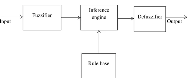
 Fuzzy inference system

A fuzzy inference system (FIS) essentially defines a nonlinear mapping of the input data vector into a scalar output using fuzzy rules.This mapping process involves:

I. input/output membership functions, II. Fuzzy Logic operators,

III. fuzzy if–then rules,

IV. aggregation of output sets, and V. defuzzification

.

Input Output

FIG 2.1:-BLOCK DIAGRAM OF A FUZZY INFERENCE SYSTEM.

Fuzzifier

Inference

engine Defuzzifier

15

CHAPTER 3

16

3.1 WHY WAVELET TRANSFORM METHOD?

1. The main idea of this method is to look at the signal at different scales or resolution. 2. The generated signals are decomposed through wavelet transform and any change in

smoothness of the signal is detected at different level. 3. Different level gives different resolution

Basically the DWT evaluation has two stages. The first stage is determination of wavelet coefficients. Those coefficients represent the signals in wavelet domain. Second stage is achieved with calculation of both the approximation and detailed coefficients. Hence this method helps both in disturbance detection as well as its location in real time[11].

3.2 DISCRETE WAVELET TRANSFORM

The DWT of a given function ‘ f ’ is given by:-

0, 0 0, , 1 1 [ ] [ ] _{j k}[ ] [ , ] _{j k}[ ] k j j k f n W j k n W j k n M   M     



 

Where j = parameter about dilation

k = parameter about position

0, [ ] j k n 

=

17

Because the sets





0, [ ] j k k z n







  are orthogonal to each other. Here the inner

product is taken to obtain the wavelet coefficients. The approximation coefficient is given by

0 0, , 1 [ ] [ ] _{j k}[ ] n W j k f n n M  



The detailed coefficient is given by

, , 0 1 [ ] [ ] j k[ ], n W j k f n n j j M  



3.3 THE FAST WAVELET TRANSFORM

If the form of scaling and wavelet function is known, its coefficients are defined in (2) and (3). , The computation time can be reduced if we can find another way to find the coefficients without knowing the scaling and dilation version of scaling and wavelet function[12].

/2 , ( ) 2 (2 ) J J j k t t k     (3.4) /2 , ( ) 2 (2 ) J J j k t t k     (3.5)

3.4 MULTI RESOLUTION SIGNALS DECOMPOSITION & ITS IMPLEMENTATION

1. In power quality disturbance signals, many disturbances contain sharp edges, transitions and jumps.

2. By using MSD techniques the power quality disturbances signals is decomposed into two signals

18

a) Smoothen version of the power quality disturbance signal

b) Detailed version of power quality disturbance signal that contains the sharp edges, transitions.

The MSD techniques discriminates disturbance from the original signal and then analysed them separately.

Let c n₀[ ] be a discrete time signal

c n₁[ ] is the smoothed version of the original signal d n₁[ ] is the detailed version of the original signal

0[ ]

c n in the form of wavelet transform coefficient can be given as

1[ ] ( 2 ) [ ]0 k c n 





Where h n( )and g n( )are the associated filter coefficients that decomposes c n₀[ ] into c n₁[ ]and 1[ ]

d n . The signal was decomposed at scale 1. For scale 2 decomposition

2[ ] ( 2 ) [ ]1 k c n 





3.5 DETECTION & LOCALIZATION OF POWER QUALITY DISTURBANCES

3.5.1 Detection

1. The filters h n( )and g n( )determines the wavelet used to analyse the signalc n₀[ ]. 2. It filters are chosen with 4 coefficients, then the Daubechis wavelet is called as Daub4.

19

3. Filters h(n) and g(n) form a family of scaling ( )t and wavelet ( )t functions i.e.

( ) 2 ( ) (2 ) n t h n t n  





The signal obtained from h n( ) is c n₁[ ], a smooth version of c n₀[ ] because h n( ) has a low frequency version.

Similarly the signal from g n( ) is the disturbance detailed signal, removed from c n₁[ ] i.e. d n₁[ ].

3.5.2 Localization

Localization of disturbance involves filtering and determination by a factor ‘2’.

1 1, 1 ( ) ( ) ( ) ( ) ( ) 2 2 n t c n f t  t dt f t  n dt     

_

_

_

_





f t =dummy signal obtained by the combination of c n₀[ ] and scaling function at scale ‘0’. Substituting (10) and (11) in (12) and (13) we get

1( ) ( ) ( ) ( 2 ) k c n f t h k  t n k   





_



20 Original Signal

[FIG 3.1 TREE DIAGRAM FOR 2-LEVEL DECOMPOSITION]

0( ) c n

g

2

2

g

2

2

21

Power Quality

Events

[FIG 3.2 BLOCK DIAGRAM OF POWER QUALITY ASSESSMENT]

3.6 TOTAL HARMONIC DISTORTION (THD)

The distortion is the measure of signal impurity. The distorted signal contains in its spectrum the harmonics that are multiples of fundamental frequency besides the fundamental component itself. The total harmonic distortion (THD) of a signal is a measurement of the harmonic distortion present and is defined as the ratio of the sum of the powers of all harmonic components to the power of the fundamental frequency. This is used to characterize the linearity of audio systems and the power quality of electric power systems.

There will be reduction in peak currents, heating, emissions, and core loss in motors in power system if THD remains low.

The WT is known as a special type of sub-band decomposition. The transform coefficients thereby obtained contain the information about different sub-band (or scale) harmonic components of the original data.

Decomposition using Wavelet Transform THD Energy Feature extracting wavelet Transform Classification using Soft Computing Techniques Type of Disturbances

22

Wavelet transform algorithm produces DWT coefficients starting from separating the original signal s of length N to 2 set of coefficients: approximate coefficients cA1 by low pass filter and detail coefficients cD1 by high pass filter. The length of each filter is equal to half of original’s length by down sampling function. The next step splits the approximate coefficients cA1 in two parts again by the same process but replace s by cA1 and producing cA2 and cD2 and so on.

Total harmonic distortion (THD) can be obtained by summating the distortion measures of different scales. It can be easily deduced that the distortion caused by each sub-band harmonics is given by the RMS value of the coefficients

2 1 [ j( )] n j RMS d n N 



Where Nj is the no of detail coefficients at scale j while THD is calculated by considering each

sub-band contribution as[14]

2 2 1 [ ( )] 1 [ ( )] j n j j n j d n N THD c n N 





The wavelet transform based method provides an alternative for harmonic analysis. With this method, distortions due to different sub-band harmonics can be easily estimated and each harmonic component can be evaluated from part of the transformed data. The accuracy achieved is satisfactory with potential of further improvement.

23

3.7 WAVELET ENERGY

If the scaling functions and wavelets form an orthogonal basis, Parseval’s theorem relates the

energy of the signal x t( ) to the energy in each of the components and their wavelet coefficients. The wavelet energy can be used to extract only the useful information from the signal about the process under study. Wavelet Energy gives the information about energy associated with the frequency bands and can detect the degree of similarity between segments of a signal[15].

2 2 2 ( ) _j( ) _j( ) k j k E







24

3.8 MAMDANI RULE BASE

The Mamdani rule based system (crisp model) takes crisp inputs and produces crisp outputs. This is done by user-defined fuzzy rules on user-defined fuzzy variables. The central idea behind using a Mamdani rule base to model crisp system behavior is that the rules for many systems can be easily described by humans in the fuzzy outputs that model system behavior; create a framework that maps crisp inputs to crisp outputs[16].

The operation of this rule base can be broken down into four parts: 1) mapping each of the crisp inputs into a fuzzy variable (fuzzification); 2) determining the output of each rule given its fuzzy antecedents; 3) determining the aggregate output(s) of all of the fuzzy rules; 4) mapping the fuzzy output(s) to crisp output(s) (defuzzification).

3.8.1 Fuzzification

First the membership of each fuzzy input variable is evaluated for the given crisp input and then the resulting value is used in evaluating the rules.

3.8.2 Evaluating the Rules

By the compositional rule of inference these rules are evaluated using the membership values of determined during fuzzification. The result is an output fuzzy set that is some clipped version on the user-specified output fuzzy set. The height of this clipped set depends on the minimum height of the antecedents.

25

3.8.3 Aggregating the Rules

After the pervious step, we have a fuzzy output defined for each of the rules in the rule base. These fuzzy outputs should combine into a single fuzzy output. The output of the rule base should be the maximum of the outputs of each rule.

In determining the system behavior the another thing to consider is that some rules might be more important than other rules. To account for this, our rule base allows the user to define a weight to each of the rules. By this the maximum weight is one and the minimum weight is zero. The fuzzy output of each rule is then multiplied by its weight.

3.8.4 Defuzzification

After the pervious step, we have a fuzzy output defined for the rule base. This output should be converted into a crisp output. Among the various types of defuzzification methods, the Centre of Area (COA, or Centroid) and Maximum are the two most widely used techniques. The COA derives the crisp number by calculating the weighted average of the output fuzzy set while the Maximum method chooses the value with maximum membership degree as the crisp number.

3.8.5 Centroid defuzzification method

In this method, the defuzzifier determines the centre of gravity (centroid) yi’ of B and uses that

value as the output of the FLS. The centroid for a continuous aggregated fuzzy set is given by

( ) ' ( ) i B s B s y y dy y y dy   





26

Where S denotes the support of µB(y). Often, discretized variables are used so that y’ can be

approximated as shown in Equation (5), which uses summations instead of integration in terms of fuzzy variables.

Mamdani rule base designing requires three steps: 1) determine appropriate fuzzy sets over the input domain and output range; 2) determine a set of rules between the fuzzy inputs and

1 1 ( ) ' ( ) n i B i i n B i i y y y y     





The centroid defuzzification method finds the “balance” point of the solution fuzzy region by calculating the weighted mean of the output fuzzy region. It is the most widely used technique because the defuzzified values tend to move smoothly around the output fuzzy region when it is used.

27

CHAPTER 4

RESULTS

AND

28

4. WAVELET DECOMPOSITION OF DISTURBANCE SIGNAL

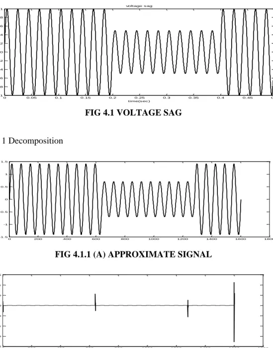
4.1 Voltage Sag: sudden drop of voltage magnitude from its nominal value typically lasting from a cycle to a second

FIG 4.1 VOLTAGE SAG

4.1.1 Level 1 Decomposition

FIG 4.1.1 (A) APPROXIMATE SIGNAL

FIG 4.1.1 (B) DETAILED SIGNAL.

0 0.05 0.1 0.15 0.2 0.25 0.3 0.35 0.4 0.45 0.5 -1 -0.8 -0.6 -0.4 -0.2 0 0.2 0.4 0.6 0.8 1 time(sec) ma gn itu de (vo lts ) voltage sag 0 200 400 600 800 1000 1200 1400 1600 1800 -1.5 -1 -0.5 0 0.5 1 1.5 0 200 400 600 800 1000 1200 1400 1600 1800 -0.02 -0.015 -0.01 -0.005 0 0.005 0.01 0.015

29

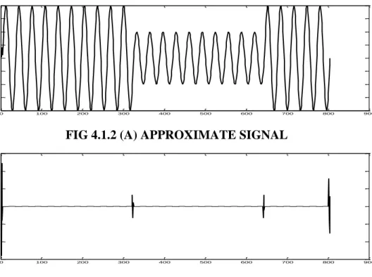
4.1.2 Level 2 Decomposition

FIG 4.1.2 (A) APPROXIMATE SIGNAL

FIG 4.1.2 (B) DETAILED SIGNAL.

4.1.3 Level 3 decomposition

FIG 4.1.3(A) APPROXIMATE SIGNAL

0 100 200 300 400 500 600 700 800 900 -2 -1.5 -1 -0.5 0 0.5 1 1.5 2 0 100 200 300 400 500 600 700 800 900 -0.06 -0.04 -0.02 0 0.02 0.04 0.06 0 50 100 150 200 250 300 350 400 450 -3 -2 -1 0 1 2 3

30

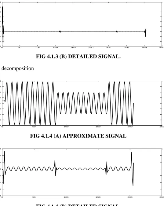
FIG 4.1.3 (B) DETAILED SIGNAL. 4.1.4 Level 4 decomposition

FIG 4.1.4 (A) APPROXIMATE SIGNAL

FIG 4.1.4 (B) DETAILED SIGNAL.

0 50 100 150 200 250 300 350 400 450 -0.15 -0.1 -0.05 0 0.05 0.1 0.15 0.2 0.25 0.3 0 50 100 150 200 250 -4 -3 -2 -1 0 1 2 3 4 0 50 100 150 200 250 -0.4 -0.3 -0.2 -0.1 0 0.1 0.2 0.3

31

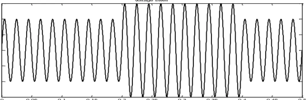
4.2 Voltage Swell: Sudden rise of voltage magnitude from its nominal value typically lasting from a cycle to a second

FIG 4.2 VOLTAGE SWELL

4.2.1 Level 1 Decomposition

FIG 4.2.1 (A) APPROXIMATE SIGNAL

FIG 4.2.1 (B) DETAILED SIGNAL

0 0.05 0.1 0.15 0.2 0.25 0.3 0.35 0.4 0.45 0.5 -1.5 -1 -0.5 0 0.5 1 1.5 time(sec) ma gn itu de (vo lts ) voltage swell 0 200 400 600 800 1000 1200 1400 1600 1800 -2.5 -2 -1.5 -1 -0.5 0 0.5 1 1.5 2 2.5 0 200 400 600 800 1000 1200 1400 1600 1800 -0.02 -0.015 -0.01 -0.005 0 0.005 0.01 0.015

32

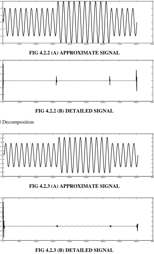
4.2.2 Level 2 Decomposition

FIG 4.2.2 (A) APPROXIMATE SIGNAL

FIG 4.2.2 (B) DETAILED SIGNAL

4.2.3 Level 3 Decomposition

FIG 4.2.3 (A) APPROXIMATE SIGNAL

FIG 4.2.3 (B) DETAILED SIGNAL

0 100 200 300 400 500 600 700 800 900 -3 -2 -1 0 1 2 3 0 100 200 300 400 500 600 700 800 900 -0.06 -0.04 -0.02 0 0.02 0.04 0.06 0 50 100 150 200 250 300 350 400 450 -5 -4 -3 -2 -1 0 1 2 3 4 5 0 50 100 150 200 250 300 350 400 450 -0.15 -0.1 -0.05 0 0.05 0.1 0.15 0.2 0.25 0.3

33

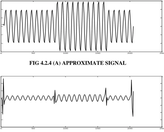
4.2.4 Level 4 Decomposition

FIG 4.2.4 (A) APPROXIMATE SIGNAL

FIG 4.2.4 (B) DETAILED SIGNAL.

0 50 100 150 200 250 -6 -4 -2 0 2 4 6 0 50 100 150 200 250 -0.4 -0.3 -0.2 -0.1 0 0.1 0.2 0.3

34

4.3 CHOICE OF DECOMPOSITION LEVEL

The different disturbances are studied with different level. Normally, one or two scale signal decomposition is adequate to discriminate disturbances from their background because the decomposed signals at lower scales have high time localization. In other words, high scale signal decomposition is not necessary since it gives poor time localization. In this case the different power quality disturbances are decomposed up to 4th level for detection purpose[17].

4.4 CHOICE OF MOTHER WAVELET

Daubechies wavelets with 4, 6, 8, and10 filter coefficients work well in most disturbance cases. Based on detection problem power quality disturbances can be classified into two types, fast and slow transients.in the fast transient case waveforms are marked with sharp edges, abrupt and rapid changes, and a fairly short duration in time. In this case Daub4 and Daub6 gives good result due to their compactness.in slow transient case Daub8 and Daub10 shows better performance as the time interval in integral evaluated at point n is long enough to sense the slow changes.

4.5 IMPLEMENTATION OF FUZZY LOGIC

Two very distinctive features like THD and ENERGY which is inherent to each disturbance is calculated.A database of THD and ENERGY of each disturbance at various degree/intensity is prepared. Now based on this database a fuzzy logic system is implemented to classify different power quality disturbances.

35

TABLE 4.3 DATA BASE OF FEATURES EXTRACTED

Type of fault Range of fault Range of Energy Range of THD

Interruption 1% to 9% of fault 972.2988 to 982.5388 (E1) 0.7424 to 0.7467(thd3) Sag 10% to 90% of fault 978.5708 to 1490.6 (E2) 0.7411 to 0.7464(thd2). Surge 160% to 240% of fault 1615.5 to 1618.7 (E3) 0.8011 to 0.8113(thd4) Swell 110% to 190% of fault 1746.6 to 3282.6 (E4) 0.7373 to 0.7399(thd1) Interruption with harmonics 3rd, 5th and 7th 2653.8 to 2752 (E5) 0.9 to 1.73(thd5)

Sag with harmonics 3rd, 5th and 7th 2660.1 to 3260 (E6) 0.9 to 1.73(thd5) Swell with harmonics 3rd, 5th and 7th 3428.1 to 5052 (E7) 0.9to 1.73(thd5)

36

4.5.1 RULE BASE

There are total 35(i.e. 7*5) number of rules. Out of these only 7 rules are feasible.

From the above database following 7 rules are formed for classification purpose.

Rule1: If Energy is E1 and THD is thd3 then disturbance is Interruption.

Rule2: If Energy is E2 and THD is thd2 then disturbance is Sag.

Rule3: If Energy is E3 and THD is thd4 then disturbance is Surge.

Rule4: If Energy is E4 and THD is thd1 then disturbance is Swell.

Rule5: If Energy is E5 and THD is thd5 then disturbance is Interruption with harmonics.

Rule6: If Energy is E6 and THD is thd5 then disturbance is Sag with harmonics.

37

FIG 4.3:-FIS EDITOR WINDOW FOR PQ DISTURBANCES CLASSIFICATION

System dist: 2 inputs, 2 outputs, 7 rules thd (5) energy (7) type (4) output2 (2) dist (mamdani) 7 rules

38

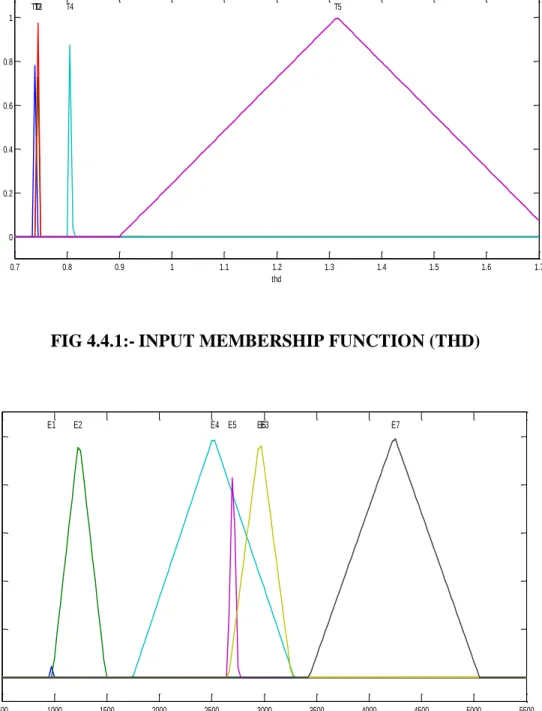
FIG 4.4.1:-INPUT MEMBERSHIP FUNCTION (THD)

FIG 4.4.2:-INPUT MEMBERSHIP FUNCTION (ENERGY)

0.7 0.8 0.9 1 1.1 1.2 1.3 1.4 1.5 1.6 1.7 0 0.2 0.4 0.6 0.8 1 thd D e g re e o f m e m b e rs h ip T1T2T3 T4 T5 500 1000 1500 2000 2500 3000 3500 4000 4500 5000 5500 0 0.2 0.4 0.6 0.8 1 energy D e g re e o f m e m b e rs h ip E1 E2 E4 E5 E6E3 E7

39

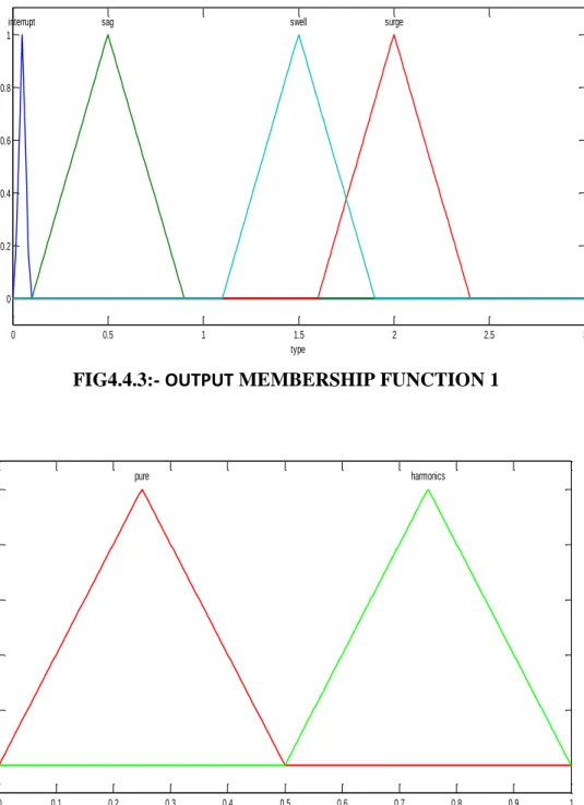
FIG4.4.3:- OUTPUT MEMBERSHIP FUNCTION 1

FIG 4.4.4:- OUTPUT MEMBERSHIP FUNCTION 2

0 0.5 1 1.5 2 2.5 3 0 0.2 0.4 0.6 0.8 1 type D e g re e o f m e m b e rs h ip

interrupt sag swell surge

0 0.1 0.2 0.3 0.4 0.5 0.6 0.7 0.8 0.9 1 0 0.2 0.4 0.6 0.8 1 output2 D e g r e e o f m e m b e r s h ip pure harmonics

40

FIG 4.5:-SURFACE PLOT OF FIS

. 0.7 0.8 0.9 1 1.1 1.2 1.3 1.4 1.5 1.6 1.7 500 1000 1500 2000 2500 3000 3500 4000 4500 5000 5500 0.5 0.6 0.7 0.8 0.9 1 1.1 1.2 1.3 1.4 1.5 thd energy t y p e

41

42

CHAPTER 5

CONCLUSION

&

43

5.1 CONCLUSION

Electric power quality is often severely affected by harmonics and transient disturbances which is a current interest to several power utilities all over the world [18]. Power quality is becoming an important and challenging issue for the power engineers due to increased use of various power electronic devices in modern power systems. This article presents some of the challenges in applying signal processing techniques to PQ disturbance recordings. A Wavelet Transform technique for analysis of PQ disturbances is presented in this paper. Waveform distortion type of PQ disturbances has been discussed and deliberated. Different types of disturbance signals are generated in the process of computation. The computational results have shown that MATLAB is a suitable tool to create PQ disturbances artificially. A fuzzy logic-based classifier is designed and integrated in the structure developed for power analysis and monitoring. To keep the analysis simple and understandable, only three types of voltage quality problems are considered: voltage sags/swells and harmonics. A limited number of rules are based on triangular membership function.

5.2 FUTURE WORK

This research work is suitable for the 50 Hz fundamental power frequency. If the system fundamental frequency is not equal to 50 Hz, then above all the procedures will not work. In that case we have to go for alternative methods for PQ assessment. Besides this there are other problems are present. The work for some other PQ disturbances should be done in future. Here only two features are extracted for the classification of PQ distortion. But more number of features can be calculated which will be helpful for accurate classification. Classification accuracy work can be done in future also.

44

REFFERENCES

[1] Watson N.R., Arrillaga J., and Chen.S., 2000b. Power system quality assessment, John Wileyand Sons Ltd., London.

[2] https://lirias.kuleuven.be/bitstream/1979/278/2/PhDThesisCristinaGherasim.pdf.

[3] R. C. Dugan, M. F. McGranaghan, S. Santoso, and H. W. Beaty, Electrical Power Systems Quality, 2nd edition, New York: McGraw-Hill, 2003.

[4] Karthik, N.,

“

[5] http:// www.standards.ieee.org.

[6] Y. H. Gu “Bridge the gap: signal processing for power quality applications,” Electrical Power System Research Journal, vol. 66, no. 1, pp. 83–96, 2003.

[7] M. Wang, G. I. Rowe, and A. V. Manishev, “Classification of power quality events using optimal time-frequency representations, theory and application,” IEEE Trans. Power Del., vol. 19, no. 3, pp. 1496–1503, Jul. 2004.

[8] Zadeh, L. A., 1994. Fuzzy logic, neural networks and soft computing. Communications of the ACM, vol. 37, pp. 77–84.

[9]Wang, Li-Xin and Mendel, J. M., 1991. Generating fuzzy rules by learning from examples. Proceedings of the IEEE International Symposium on Intelligent Control, Arlington, VA, pp. 263–268.

[10] Mendel, J. M., 1995. Fuzzy logic systems for engineering: A tutorial. Proceedings of the IEEE, vol. 83, no. 3, pp. 345–377.

45

[11] Z.-L. Gaing, “Wavelet-based neural network for power quality disturbance recognition and classification,” IEEE Trans. Power Del., vol. 19, no. 4, pp. 1560–1568, Oct. 2004.

[12] R. Polikar, The Engineer’s Ultimate Guide to Wavelet analysis, The Wavelet Tutorial.March 1999.

[13] Choudhury, Debasis , “Power quality event monitoring and characterization using Wavelet based fuzzy expert system”, 1st National Conference on Power Electronics Systems & Applications, PESA 2013.

[14] S. Tuntisak and S. Premrudeepreechacharn, “Harmonic Detection in Distribution System Using Wavelet Transform & Support Vector Machine”,IEEE Conference on Power Tech 2007.

[15] J.S. Huang, M. Negnevitsky and D.T. Nguyen, “Wavelet transform based harmonic analysis,” Australasian universities power engineering Conference and IE Aust Electric Energy

Conference, pp.152-156, 1999.

[16]L. A. Zadeh. Fuzzy logic. IEEE Computer, 21(4):83–93, April 1988. [17]Wavelet Toolbox User’s Guide.

[18] D. Saxena, K.S. Verma and S.N. Singh, Power quality event classification: an overview and key issues, International Journal of Engineering, Science and Technology Vol. 2, No. 3, 2010.