CEDA 3.0 User s Guide

(1)

CEDA 3.0 User’s Guide January 2004

CML, Leiden University, PO Box 9518, 2300RA Leiden, The Netherlands

CEDA/3.001/01/2004

CEDA 3.0

User’s Guide

Leiden University Institute of Environmental Science (CML)

Sangwon Suh*

CML, Leiden University

Leiden, The Netherlands

* Currently at

College of Natural Resources

University of Minnesota

Minnesota, USA

[email protected]

(2)

(3)

CEDA/3001/01/2004

CEDA 3.0 User’s Guide

A Comprehensive Environmental Data Archive for Economic and Environmental Systems Analysis

CEDA 3.0 contains

Resources Consumption • Greenhouse Gas Emissions • Land Use • Toxic Emissions • Particulate Matter Emissions

• Pesticide Use • Ozone Depleting Substance Emissions • Nutrient Emissions • Energy use

by 480 US commodities and services

For use in

Environmental and Economic Policy Modeling • Integrated Product Policy • Screening and Hybrid Life Cycle Assessment • Environmental Input-Output Analysis •

Material Flow Analysis • Substance Flow Analysis •

Analysis of Environmental Impacts of Products and Services • Environmental Design.

CEDA 3.0 User’s Guide

by Sangwon Suh

(4)

Leiden University, The Netherlands.

CEDA/3001/01/2004

This guide may be freely distributed provided the source is clearly indicated. http://www.leidenuniv.nl/cml/ssp/index.html

http://www.EnviroInformatica.com/ceda/index.html Part of this guide has been published as

Suh, S., 2005: Developing Sectoral Environmental Database for Input-Output Analysis: Comprehensive Environmental Data Archive of the U.S., Economic Systems Research, 17 (4), 449 – 469

Last modified: Feb. 2006

CEDA 3.0 was developed in collaboration between

CML, Leiden University EnviroInformatica, Co.

PO Box 9518, 2300RA 710-1201, Manhyun-dong, Yong-In Leiden, The Netherlands. Kyonggi-do, South Korea. http://www.leidenuniv.nl/cml http://www.EnviroInformatica.com

[email protected]

Distributed by

EnviroInformatica, Co.

710-1201, Manhyun-dong, Yong-In Kyonggi-do, South Korea.

http://www.EnviroInformatica.com [email protected]

(5)

1. What is CEDA 3.0 ?

1.1. A brief background

CEDA 3.0 is the successor of MIET 2.0, a missing inventory estimation tool for Life Cycle Assessment (LCA) developed by CML (Suh 2001, Suh and Huppes, 2002). Over 500 MIET users worldwide have registered since its first release in 2001. In 2004 MIET 2.0 was updated to MIET 3.0, which has substantially improved data quality by using additional data sets and the most up-to-date data sources and is now included in the standard data package SimaPro, an LCA software tool by PRé Consultants. There are many MIET users who are not LCA practitioners, however, and who wish to continue using the MIET package. These users have been applying MIET for various kinds of analysis, including environmental and economic policy modeling, Integrated Product Policy (IPP), environmental Input-Output Analysis (IOA), Material Flow Analysis (MFA), Substance Flow Analysis (SFA), analyses of consumption and its environmental impacts, and alternative material selection in environmental design. Furthermore, some of the LCA users were keen to see an easy-to-use software tool with which to quickly access detailed data and perform a number of essential analyses for screening and hybrid LCAs. To satisfy the needs of both LCA practitioners and other MIET users, the software tool CEDA 3.0 described in this User’s Guide was designed by EnviroInformatica, Co., an environmental data processing and warehousing company.

1.2. What kinds of data sets does CEDA 3.0 contain?

CEDA 3.0 comprises three main database modules: (1) an economic input-output database module, (2) an environmental intervention database module, and (3) a characterization factor database module for impact assessment.

The input-output database module is derived from a variety of economic statistics, including 1998

US make and use accounts, the 1992 US capital flow matrix, a standard comparison table between US Standard Industry Classification (SIC) codes and the input-output industry codes of the US Bureau of Economic Analysis (BEA), and producer’s price change data from the US Bureau of Labor Statistics (BLS). The input-output data module contains information on the structure of inter-industry exchanges of materials and energy throughout the supply chains for

(8)

production and consumption of 480 commodities and services in the US. The level of resolution of US input-output statistics is among the best in the world, and they encompass a great many of the production technology mixes in widespread use today. The commodity

categories included in the input-output data module are listed in Appendix A.

The environmental intervention database module contains information on generation of 1344

environmental interventions. It is derived from various environmental databases, including the Toxics Releases Inventory (TRI), National Toxics Inventory (NTI), National Environmental Trend (NET) databases, greenhouse gas emissions and sinks data, agricultural chemical and fertilizer use data, mineral and fossil fuel resource use database, energy consumption data, and land use data from the US. Data sources include the Census Bureau (2001), the Environmental Protection Agency, the Energy Information Administration of the Department of Energy, the National Agricultural Statistics Service and Natural Resources Conservation Service of the Department of Agriculture, the National Center for Food and Agricultural Policy, and the United States Geological Survey. The interventions covered include resource use (6 items), land use (1 item), and environmental emissions to air (551 items), to freshwater (331 items), to industrial soil (236 items), and to agricultural soil (219 items) and relate to over 480 commodities produced in the US. The environmental interventions compiled in CEDA 3.0 are the main driving causes of major environmental impacts such as global warming, ozone layer depletion, various toxic impacts to humans and ecosystems, acidification, eutrophication, land use, resource depletion, etc. A full list of the environmental interventions covered is provided in Appendix B.

Lastly, for a total of 1700 environmental interventions employed in 86 widely referenced

methods of environmental impact assessment, the characterization factor database module contains

characterization factors that allow users to aggregate environmental interventions into environmental impact scores. The selected impact assessment methods include Global Warming Potentials (GWPs), Ozone Depleting Potentials (ODPs), CML2002 methods and Eco-Indicator 99 methods. A description of environmental Life Cycle Impact Assessment (LCIA) methods, including those selected for inclusion in CEDA 3.0, can be found in Guinée

et al. (2002). A complete list of selected characterization methods is provided in Appendix C.

1.3. What kind of analysis can CEDA 3.0 do?

Users can employ CEDA 3.0 to calculate the overall, economy-wide environmental interventions generated throughout an economy in producing a certain product or service by simply searching or browsing the name of the product or service and entering its price in

monetary terms. In the context of an LCA, this result is generally termed the inventory result.

Users may enter the price as either a producer’s or a consumer’s price, but need to specify which it is. If entered as a consumer’s price, CEDA 3.0 automatically converts it to a producer’s price based on the commodity-specific transportation cost and retail and wholesale margins. The inventory result can be exported to a spreadsheet. Users can then quantify the environmental impacts of the product or service throughout an economy by choosing the

(9)

User’s guide

option “Environmental Impact Assessment”. CEDA 3.0 then matches relevant impact assessment factors with the inventory result to calculate the sum total of environmental

impacts. This result is generally referred to as the characterized result. The operational procedure

for generating characterized results is as simple as that for inventory results, and the results can again be exported to a spreadsheet or text file.

CEDA 3.0 performs contribution analyses for both inventory results and characterized results. A typical contribution analysis identifies those products and services whose direct generation of environmental interventions or impacts contributes most to the total in the supply chain of the product or service under study. With the results of a contribution analysis users can pinpoint key contributing processes in a given supply chain. This type of contribution analysis

will be referred to here as output contribution analysis. CEDA 3.0 performs output contribution

analysis for all interventions or impact assessment methods simultaneously and once more exports the results to a spreadsheet or text file.

CEDA 3.0 is also capable of another powerful kind of contribution analysis: input contribution

analysis (Suh, 2003a; Suh 2003b). The products or services identified in an output contribution

analysis as being key upstream contributors may be rooted in still higher upstream processes over which the producer of the product or service under study has no control. A practical issue for producers is then the extent to which their environmental performance can be reduced by sourcing input materials from alternative suppliers. Input contribution analysis therefore seeks to identify which direct inputs to the product or service under study are responsible for the greatest environmental intervention or impact through their upstream supply chains. By performing a series of input contribution analyses users can gain detailed insight into the structure of the environmental interventions or impacts induced through the supply-demand structure of a given product system. Such analyses have a variety of uses, including setting data collection priorities and initial system boundary setting for a product LCA, screening alternative production materials and other applications in the field of industrial ecology.

CEDA 3.0 can also be directly used for tiered hybrid LCA (Suh and Huppes, 2002; Suh et al.,

2004). By adding particular inventory or impact assessment results beyond the cut-off point of an existing LCA result, users can expand the system under analysis towards national borders for little extra expenditure of time or resources. By employing CEDA 3.0 at the outset of an LCA study, users can make more efficient use of the time and resources available for data collection through a process of iterative screening, collecting data on the key processes identified and performing a hybrid LCA.

CEDA 3.0 also provides data export functions, permitting advanced analysis of basic data sets using professional software packages such as MatLab and Mathematica.

(10)

2. CEDA 3.0 Methodology

2.1. Introduction

CEDA 3.0 utilizes a standard input-output framework and environmental life cycle impact assessment methods for analyzing product and service supply chains and quantifying their environmental impacts, respectively. Some of the basics of Input-Output Analysis (IOA), LCA computations and basic analyses facilitated by CEDA 3.0 are described below. For more details of IOA and LCA, however, the reader is referred to the literature referenced at the end

of this guide, e.g., Miller and Blair (1985), Heijungs and Suh (2002), and Guinée et al. (2002).

2.2. Input-Output Analysis

Leontief multiplier

Input-output analysis reveals how industries are interlinked through chains of commodity supply and usage. Its basic point of departure is an input-output coefficient table, derived from inter-industry transaction records, in which each column cites coefficients representing the relative amount of inputs required to produce one dollar’s worth of output of the industry in question. In fixing these coefficients it is assumed that any magnitude of output of the given industry will require inputs from other industries proportional to these coefficients. This is the proportionality assumption of conventional input-output analysis. The question is then: what amount of inputs is required to meet final demand for the product? This cannot be readily answered by a few simple steps of addition, since every industrial output required for producing a given product requires outputs from other industries, too, and so on. If every

industry has N inputs, then the number of input paths on the kth tier will be Nk_.

W. Leontief elegantly solved this problem by introducing a few assumptions and a simple matrix inversion known as a Leontief multiplier (Leontief 1970). Leontief’s solution can be summarized as a system of non-homogeneous equations (1).

(11)

User’s guide (1) . n n n nn n n n n n n n y y y x a x a x a x a x a x a x a x a x a x x x M M L O L L M M M 2 1 2 1 2 2 2 22 2 12 1 1 1 21 1 11 2 1 + + + + + + + + + + + + = = =

The ith element of x, x_i is the total annual output of the ith industry, while a_ij stands for the

fractional output of the ith industry consumed by the jth industry in producing one unit of its

output. It is assumed in IOA that the coefficients aij are fixed, i.e., the ‘recipe’ of each product

or service remains unchanged regardless of the volume of production. Thus, aijxj gives the

fraction of ith industry output consumed in producing the total annual output of the jth

industry. The ith element of the last column, yi is the quantity of ith industry output consumed

by households. Overall, equations (1) represent the supply-demand balance of a national economy, where total annual production equals total consumption by industry plus total

consumption by households.1

Using matrices and vectors the equations (1) can be rewritten as:

(2) x=Ax+y,

which can be rearranged into:

(3) x I A 1y.

) ( − −

=

The inverse matrix in equation (3) is referred to as a Leontief multiplier and it represents the

amount of industry output required directly or indirectly through supply chains to produce one unit of each industry output. The Leontief multiplier permits a variety of economy-wide

analyses to be carried out. For instance, the economy-wide primary energy requirement e

required to meet an arbitrary final demand y is calculated as:

(4) e=εˆ(I−A)−1y,

where denotes a diagonalized vector of direct energy input to each industry per dollar’s worth of output of each sector. If good detailed statistics are available, input-output analysis can yield reliable information on the economy-wide use of energy, employment, resources, water, etc. industries.

εˆ

Supply and use framework

(12)

The aggregate direct and indirect requirements of industrial output for meeting a given final demand, calculated using equation (3), provide no information on individual ‘commodity’ requirements. Industries generally produce more than one product and depending on the industry in question the amount of secondary and tertiary products may be considerable. The ‘supply and use’ framework provides a methodological basis for dealing with commodities in

input-output systems (Stone et al., 1963).

Since the introduction of the System of National Accounts (SNA) (United Nations 1968), many countries have employed this supply and use framework for their national accounts system. Since 1972, US DOC has prepared supply and use matrices and used these to derive a total requirement matrix. The usefulness of the supply and use framework is dual. First, the method greatly improves statistical quality, because the products and services consumed and produced by each individual establishment are better known than the sectors to which they belong. Second, the framework makes an explicit distinction between commodity output and industry output permitting appropriate treatment of secondary products and scrap (Konijn, 1994).

CEDA 3.0 utilizes a commodity × commodity total requirements matrix derived from 1998

supply and use matrices using an industry-technology model. The general calculus used to derive the total requirement matrix is shown in BEA (1995b).

2.2. Life Cycle Assessment

LCA is widely used for assessing the environmental aspects of a product or service. LCA consists of four major steps: goal and scope definition, inventory analysis, impact assessment and interpretation (ISO, 1998). In the goal and scope definition phase, the objective of the study, its intended application, the required data quality, system boundary and so on are set. In the inventory analysis phase, data on environmental interventions are collected or calculated, on-site from an appropriate industry or using LCA databases, respectively. In Life Cycle Inventory (LCI) analysis, the computational algorithm is also based on matrix inversion and is essentially the same as that used in IOA (Heijungs and Suh, 2002). In the impact assessment phase, the environmental impacts of the product or service are assessed by multiplying LCI results by relevant characterization factors quantifying the relative contribution of each environmental intervention to a particular environmental impact category such as global

warming or ozone layer depletion (Guinée et al., 2002). To arrive at more aggregate indicators,

this ‘characterization’ step may be followed by a number of additional steps, including normalization, grouping and weighting. These post-characterization steps are not incorporated in CEDA 3.0 but may be pursued by individual users.

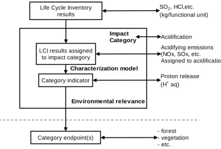
The characterization step is dealt with in more detail below. The notion of characterization has been developed independently within several scientific communities. In LCA, Global Warming Potentials (GWPs) and Ozone Depleting Potentials (ODPs) are among the most familiar characterization indicators currently employed. Once generated, any environmental

(13)

User’s guide

intervention goes through a series of physical and chemical processes before eventually

culminating an environmental problem. For instance, SO2 emissions combine with water to

form H₂SO₄, which may be ionized to 2H+_{and SO}

42-. As precipitation transfers these

hydrogen ions to the soil system and lowers soil pH, the resultant acidification process may impact on vegetation and forestry. Together, these successive processes are referred to as an environmental mechanism. Some environmental mechanisms are fairly simple, but most are complex and involve a multitude of physical and chemical transformations and fate and exposure routes. In an LCIA, a category indicator is chosen along with the environmental mechanism in such a way that the indicator reflects an important causal and quantitative relationship with the category endpoint. For instance, the total number of hydrogen ions generated in the process of acidification may provide a good category indicator. Using selected category indicators, each environmental intervention can be represented in terms of its equivalence to a reference intervention in the impact category in question. In the case of global warming, for instance, the radiative force of each greenhouse gas is chosen as category

indicator (termed Global Warming Potential) and CO₂ as reference intervention for 1 GWP.

Characterization model

LCI results assigned to impact category Category indicator Life Cycle Inventory

results Category endpoint(s) SO2, HCl,etc. (kg/functional unit) Acidification Acidifying emissions (NOx, SOx, etc.

Assigned to acidification) Proton release (H+ aq) Example - forest - vegetation - etc. E n vi ro n m en ta l M e c h a n is m Impact Category Environmental relevance

Figure 1. Concept of category indicators (ISO, 1999)

Characterization factors are simply a set of factors for converting LCI results into the equivalent terms of a reference intervention. Depending on the characterization model used, the time horizon considered and the physical location of the category indicator, however, a number of different approaches are available to this end. The 86 methods included in CEDA 3.0 cover and embrace the characterization factor sets that are most widely referenced and are linked internally to all other interventions to avoid errors in linking interventions with appropriate factors.

(14)

2.3. Basic analytical tools of CEDA 3.0

This section describes the basic analytical tools incorporated in CEDA 3.0. Non-technical users may skip this section.

Let k and j index commodity, i environmental intervention, and h impact category. Let A be

the commodity-by-commodity input-output structural coefficient matrix or direct

requirements matrix, with an element of A, ajk denoting the amount of j directly required to

produce one unit of k. In CEDA 3.0 imports and capital flows are endogenized in the direct

requirements matrix A. Let B be the environmental intervention matrix, with an element of B,

bij denoting the amount of i generated or required to produce one unit of j. Let y denote final

demand, with an element of y, yk denoting final demand for k. In general, the overall

environmental interventions generated due to final demand y is then calculated as

(4) m B I A 1y.

) ( − −

=

The column vector m has a dimension of i × 1 and represents the overall environmental

interventions generated directly and indirectly by industry in supplying the final demand y (cf.

equation (3)). In an LCA context, m is regarded as an inventory of the ‘functional unit’ satisfied

by y. The final demand y can be entered as either a producer’s or consumer’s prices. If users

know the exact 1998 producer’s price of the commodity at stake, they can enter the price by selecting “Producer’s price” in the dialogue box. A set of default conversion factors devised

for CEDA 3.0 convert consumer’s prices into producer’s prices. The vector m is the

calculation result that a user will see having chosen the “Inventory” radio button in the workspace. CEDA 3.0 allows only one final demand item to be entered at a time; an inventory comprising multiple final demand items can be calculated by running the query a number of times and summing the results.

If desired, users can also perform a contribution analysis by clicking either “Input contribution” or “Output contribution” in the dialog box “Results”. One key question addressed by LCA contribution analysis is “what environmental interventions (or environmental impacts) are generated in which upstream or downstream processes?”, providing insight into key indirect contributors to supply-chain burden. This type of analysis

will be referred to here as output contribution analysis (cf. Suh, 2004; Heijungs and Suh, 2002).

Using the above formula and definition, the output contribution is calculated as

(5) M B I A 1y . , ) ( − Ω ₌ ₋ i i _,

where B_i_.is a diagonalized ith row of B, and represents the contributions of each

commodity to environmental intervention i. As CEDA 3.0 calculates the contributions of all

relevant commodities to all environmental interventions, the dimension of the resultant matrix

i ,

Ω

(15)

User’s guide

is rather large. Consequently, the result of a contribution analysis is not displayed but can be exported to spreadsheet or text format for further analysis by users. Although output contribution analysis is eligible as a method for identifying upstream and downstream processes that generate significant environmental interventions, it does not indicate which particular direct inputs to the commodity under study are responsible for inducing them. This information may be sought by users in order to prioritize input materials and the processes

using them for further improvement. This type of analysis is referred to in this manual as input

contribution analysis (cf. Suh, 2003a; Suh, 2004).

The input contribution is calculated as

(6) M B I A 1Ay . , ) ( − Α ₌ ₋ i i ,

where Ay is a diagonalized column vector, Ay, and is the contribution to the

environmental intervention i .

i ,

Α

M

As the number of environmental interventions covered by CEDA 3.0 is rather large and the same chemical may have several different names, matching inventory results with characterization factors can be a time-consuming job and may create additional errors. For this reason CEDA 3.0 links the inventory results with 86 of the most widely referenced characterization methods. The links between environmental interventions and characterization factors are established internally using Chemical Abstract Service (CAS) numbers and own identifiers, as follows.

Let h index characterization methods and C be the characterization factor matrix, where an

element of C, chi represents the characterization factor for environmental intervention i in

characterization method h. A characterized result is then calculated as

(7) q CB I A 1y.

) ( − −

=

As with the inventory results, users can perform an additional contribution analysis on the characterized results. The equation

(8) Q CB I A 1y . , ) ( ) ( − Ω ₌ ₋ h h _,

where (CB)h. is a diagonalized hth row of CB, calculates the output contribution using

characterized results. Input contributions are calculated as

(9) Q CB I A 1Ay . , ) ( ) ( − Α ₌ ₋ h h

(16)

2.4. Derivation of environmental matrix

A detailed description of the data used for the environmental database module as well as their respective sources is provided in the next chapter. In this section we deal, in brief, with the computational aspect only.

Generally speaking, the overall economy-wide direct and indirect environmental interventions

caused by a given final demand for commodity y is calculated by means of equation (4). Since

a commodity × commodity matrix is utilized for the input-output part, the dimension of M

should likewise be intervention × commodity. For instance, the equation

(10) m* =BI(I−A)−1y,

where BI_{is the environmental intervention}_×_{industry matrix representing the overall}

environmental interventions caused by the production of 1 dollar’s worth of industry output, encountered in some of the literature, is not in fact congruent.

The consequence of the confusion between industry and commodity in equation (10) may be significant, at least in the US, where the proportion of secondary products produced in each industry is considerable (Miller and Blair, 1985). According to the recent input-output table prepared by BEA, up to 77.8% of the market share of each commodity is dependent on industries that do not produce the commodity as a primary product. In the US economy, furthermore, the portion of secondary products generated by each industry may be up to 88.6% of total output in monetary terms. For all these multiple output processes, there thus arises the problem how to allocate environmental interventions and impacts appropriately. In

CEDA this problem is resolved by using the ‘make and use’ framework (cf. Suh and Huppes,

2002).

Equation (4), which calculates aggregate direct and indirect environmental interventions for a

given final demand, uses the intervention × commodity matrix B. However, information on

environmental interventions is compiled mainly on an industry rather than commodity basis. B

must therefore be derived from BI_{, by assigning the aggregate environmental intervention of}

each industry to its secondary products and scrap as well as its primary product. In LCAs many allocation methods have been proposed and used for ascribing particular environmental

interventions to co-products (Huppes et al. 1994; Guinee et al. 2002; Frischknecht 2000). The

allocation procedure adopted should preferably be based purely on physical causality between environmental intervention and production of secondary and primary products. As strict causality cannot always be established with any degree of precision, however, allocation based on the economic value of the products in question has therefore been widely adopted in LCAs, as the economic value of process output reflects the driving force of the processing operation in question.

(17)

User’s guide

proportionally to its primary and secondary products based on their economic value, the average environmental intervention due to a dollar’s worth of commodity can then be calculated on the basis of market share as

(11) B=BID_,

where D is a market share matrix derived from make and use matrices. Equation (11) gives the

aggregate environmental intervention by industries producing a given commodity based on market share. This method corresponds to the industry-technology assumption used for

deriving the direct requirements matrix A in CEDA 3.0.

Alternatively, one can assume that each commodity generates its own characteristic environmental interventions, irrespective of the industry producing it. Under this assumption, the total environmental intervention of a primary product of a given industry is calculated by subtracting the total environmental intervention due to secondary products, indexed to industries producing these secondary products as primary products. In LCA this method is referred to as the ‘avoided impact’ allocation method or ‘system expansion’ method and corresponds to the commodity-technology assumption in the make and use framework.

2.5. Hybrid analysis

Just about every functional output dealt with in LCA involves a near-infinite number of processes embodying both direct and indirect input/output relations. A motor vehicle, for example, is manufactured using a wide variety of parts and equipment, most of which require numerous raw and ancillary materials as well as energy, capital and so on. These interconnections, which can be seen as a ‘commodity flow web’, proliferates enormously through upstream processes, although the importance of certain flows may taper off as they become incorporated in indirect relations far upstream. In practice, most LCAs deal only with a limited number of these processes - hopefully the important ones – underlying production of a given functional output, establishing a cut-off point beyond which processes are ignored. To establish which processes are to be taken as the starting point for the subsequent iterative procedure, ISO (1998) suggests three criteria: mass, energy and environmental relevance. Of these, mass and energy are the most frequently used, although in some case studies mass has been found to be a poor indicator. In most cases environmental relevance has very limited applicability as a cut-off criterion, since the very problem in selecting ‘promising processes’ resides in the fact that the importance of flows is not usually known prior to actual collection of detailed data. The basic problem of cut-off is that we are required to choose between inputs

or outputs of which we as yet have no precise knowledge (for a detailed discussion see Suh et al.

2004).

One of the most popular ways of solving this problem proceeds from the assumption that the overall environmental significance of a process can already be reliably intimated from a few elementary traits of the process and the products it embodies. These can then be directly and

(18)

efficiently employed as cut-off criteria on for each individual process. Analyzing the simplest

such traits, mass and energy content, Raynolds et al. (2000a) concluded that these two alone

cannot generally serve as reliable indicators. In Raynolds et al. (2000a, 2000b) they found that

combining mass and energy with economic factors, yielded a more satisfactory system boundary cut-off criterion. This approach seems reasonably justified, as costs are always driven by economic activities, which are very likely to be related to environmental interventions. In view of the multitudinous origins and major variability of pollutant environmental impacts, however, generalization of the relationship between a few simple traits and overall

environmental impact based on some deductive inference seems very problematical.2_Hunt_et

al. (1998) tested 10 different methods for streamlining LCI and concluded that the validity of

any such trait can only be judged on a case-by-case basis.3

It is generally very difficult to justify omitting any flows, although this is in fact required by ISO (1998). It is therefore necessary to cover the omitted flows, rather than cut them off. On the other hand, it is impossible in practice to gather all the site-specific data associated with every single process involved in the production of a given functional output. As an alternative

to process LCA, therefore, an LCI based on IOA has been suggested (Lave et al., 1995;

Hendrickson et al., 1998). An input-output table is then prepared on the basis of national

statistics covering, in principle, all economic activities involving monetary transaction, which is thus taken to be more encompassing as a system boundary. Input-output tables have limitations of their own, however, particularly their level of resolution, which is generally too poor to be used as a full substitute for a detailed, process-level LCA.

Hybrid analysis combines process LCA (for foreground processes) and input-output LCA (for background processes) and maximizes their respective advantages of process specificity and

encompassing system boundary (Suh and Huppes, 2005; Suh, 2004; Suh et al., 2004; Joshi,

1999). There are several possible ways to combine the process LCA and IOA. The simplest of

these is tiered hybrid analysis (Bullard et al., 1978, Moriguchi et al., 1993), whereby overall

results are calculated simply by adding the results of an input-output LCA (usually only for cut-offs) to those of a process LCA. With the tiered hybrid method, users can expand the system boundary to the national economy at little additional cost. In addition, the method can be used as a screening tool for identifying further data collection priorities. As tiered hybrid analysis highlights important contributors beyond the system boundary, LCA practitioners can efficiently improve overall data quality by directing their resources first to these key contributors.

Users preferring to adopt more sophisticated analytical tools such as Monte Carlo analysis and perturbation analysis may consider performing an integrated hybrid analysis in which input-output matrix and process matrix are combined into a single matrix (Suh, 2004).

2_Raynolds_{et al}_{. also limited the area of application of their method to combustion-related emissions.}

3_{On the other hand, if there does exist a reliable indicator correlating perfectly with overall environmental impact,} it is better to use that indicator for calculating the inventory than employing a cut-off point.

(19)

User’s guide

2.6. Limitations of the CEDA 3.0 methodology

CEDA 3.0 uses US input-output accounts and LCIA methodology for its calculations, and the limitations inherent in each therefore also apply to CEDA 3.0.

Lave et al. (1995) addressed the limitations of the input-output approach for undertaking

detailed analysis. Since even the most detailed input-output tables subsume different commodities under a single classification, input-output based analysis can enable comparison at a generic, sectoral level only. Input-output based methods are therefore inadequate for

detailed process-level analysis. More fundamentally, in setting matrix A in equation (3), IOA is

based on an assumption of proportionality, i.e. it ignores both ‘economies’ and ‘diseconomies’ of scale as well as ‘the law of diminishing return’. Another source of uncertainty is discrepancy between the base year of the input-output table and that of the study. Although this kind of error can be mitigated by employing the most recently available input-output table, this may be insufficient in the case of certain rapidly changing sectors. Although input-output methods considerably extend the upstream reach of analysis, the system boundary is still not in principle truly encompassing, as the national economy is ultimately linked with international trade. For countries relying heavily on trade, truncation at the national borders may significantly reduce the usefulness of IOA. In the US, however, the amount of imports and exports is relatively small compared with domestic production, limiting possible errors due to cross-boundary commodities. In CEDA 3.0, it is assumed that imports have been produced using exactly the same technology as in the US, thus further reducing possible errors due to truncation of imports.

(20)

3. Data and data sources

3.1. Input-Output data

CEDA 3.0 uses the US 1998 annual input-output tables compiled by BEA (BEA 2002) and a calculation procedure that follows the standard US make and use framework provided in BEA

(1995a).4_{However, the 1998 annual input-output tables contain no information on capital}

flows. The most recent capital flow matrix available is for the year 1992 (BEA 1995c). Although the decision to use the 1992 capital flow table ensues largely from the problem of data availability, it is has been deemed reasonable to assume that the capital goods invested in 1992 were still in use in 1998 in most industries apart from rapidly developing sectors like the information technology (IT) sector, for which current estimates based on 1992 capital investments may be misleading. The amount of capital goods used by each sector has been inflated or deflated depending on price change information and gross output differences between 1992 and 1998 for the sector in question. In a 1992 benchmark survey by BEA, uses of 163 capital goods by 64 industries were compiled on the basis of SIC code. These have been reassigned to the relevant IO categories for inclusion in a use matrix.

In CEDA 3.0, any data involving SIC code are first assigned to the most detailed set of SIC codes, which distinguish 1037 different industries, and then reclassified under a BEA code to preserve as far as possible the detail of the primary data.

3.2. Environmental data

3.2.1. Greenhouse gas emissions

Carbon dioxide

Total US greenhouse gas (GHG) emissions, including but not restricted to carbon dioxide

(CO2) emissions, are fairly well established. Apart from the CO2 emission data for the electric

utility sector compiled by EIA and EPA, however, data at the level of individual sectors are

4_{The basic principles of input-output analysis, including the make and use framework, are summarized well in a} book by Miller and Blair (1985).

(21)

User’s guide

not readily found. Consequently, the rest of the estimation procedure for combustion-oriented

CO2 emissions focuses on other sectors than electric utility sector.

With regard to transportation, there are two categories of CO2 emissions to be distinguished:

those of domestic transportation and industrial transportation. CEDA assumes that the use of all trucks, buses, aircraft, boats and vessels and locomotives are part of industrial activities.

CO₂ emissions from international bunker fuel combustion, construction equipment and

agricultural vehicles are also assigned to industrial use. Industrial and commercial

combustion-oriented CO2 emissions have been assigned on the basis of BEA fuel use data and the data on

combustion-oriented CO2 emissions by fuel type compiled by EPA (EPA, 2002a).

Non-combustion-oriented CO₂ emissions have been assigned based on the source process cited by

EPA (2002a).

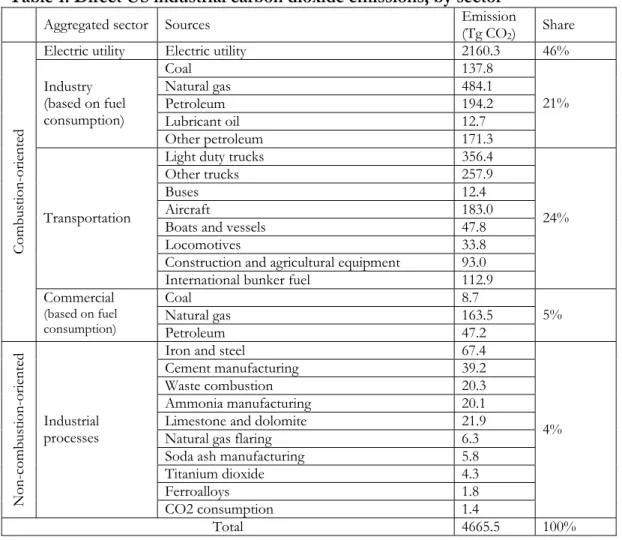
Table 1. Direct US industrial carbon dioxide emissions, by sector5

Aggregated sector Sources Emission _{(Tg CO2)} Share Electric utility Electric utility 2160.3 46%

Coal 137.8 Natural gas 484.1 Petroleum 194.2 Lubricant oil 12.7 Industry (based on fuel consumption) Other petroleum 171.3 21%

Light duty trucks 356.4 Other trucks 257.9

Buses 12.4 Aircraft 183.0 Boats and vessels 47.8

Locomotives 33.8 Construction and agricultural equipment 93.0

Transportation

International bunker fuel 112.9

24% Coal 8.7 Natural gas 163.5 Combustion-oriented Commercial (based on fuel consumption) _{Petroleum 47.2}5%

Iron and steel 67.4 Cement manufacturing 39.2 Waste combustion 20.3 Ammonia manufacturing 20.1 Limestone and dolomite 21.9 Natural gas flaring 6.3 Soda ash manufacturing 5.8 Titanium dioxide 4.3 Ferroalloys 1.8 Non-comb usti on-oriented _Industrial processes CO2 consumption 1.4 4% Total 4665.5 100%

(22)

In CEDA, the GHG emissions of the sources under the headings ‘industry’ and ‘commercial’ have been assigned to individual IO industries based on the transaction records for the commodities in question. The remaining emission sources could be allocated directly to the appropriate IO industrial sectors.

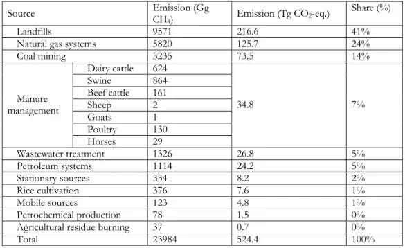
Methane

In 1998, emissions of methane (CH4) accounted for 9.3% of total industrial and households

US GHG emissions (627.1 Tg CO2-equivalents). Besides enteric fermentation (particularly by

ruminants), industrial processes such as landfills, natural gas systems and coal mining are the predominant sources, and these ‘area sources’ can be readily assigned to a relevant IO classification.

Given the CH4 emission factors for residential and commercial coal combustion (300 and 10,

respectively) and respective consumption of the two sectors in 1998 (13 Tbtu and 92 Tbtu),

based on coal consumption, only 19% of CH4 emissions from ‘stationary’ sources have been

assigned to intermediate industries (EPA 2002a and EIA 2002). According to EPA (2002a)

42% of CH4 emissions from mobile sources were due to passenger cars. Assuming other

means of transportation can be assigned to intermediate industries, 58% of ‘mobile’ CH₄

emissions can then be assigned on the basis of transportation service transaction records, and this has been done in CEDA.

Table 2. US industrial Methane emissions, based on direct emission6

Source Emission (Gg _CH4) Emission (Tg CO2-eq.) Share (%)

Landfills 9571 216.6 41%

Natural gas systems 5820 125.7 24%

Coal mining 3235 73.5 14% Dairy cattle 624 Swine 864 Beef cattle 161 Sheep 2 Goats 1 Poultry 130 Manure management Horses 29 34.8 7% Wastewater treatment 1326 26.8 5% Petroleum systems 1114 24.2 5% Stationary sources 334 8.2 2% Rice cultivation 376 7.6 1% Mobile sources 123 4.8 1% Petrochemical production 78 1.5 0% Agricultural residue burning 37 0.7 0%

Total 23984 524.4 100%

(23)

User’s guide

Nitrous oxide emissions

Because of their very minor contribution to overall GHG emissions, only two N₂O sources

have been deemed significant: ‘agricultural soil management’ and ‘mobile sources’, contributing

1.0 Tg and 0.2 Tg of CO2-equivalent GHG emissions (963 Gg and 191 Gg as N2O),

respectively. Following the same line of reasoning as for CH4, 46% of N2O emissions from

mobile sources have been assigned to intermediate industries on the basis of transportation service utilization.

Other greenhouse gas emissions

CEDA 3.0 also covers the following greenhouse gases: trichloromethane, sulfur hexafluoride, tetrachloromethane, perfluorobutane, perfluorocyclobutane, perfluoroethane, perfluorohexane, perfluoromethane, perfluoropentane, perfluoropropane, methylbromide, methyl cyclohexane, HALON-1211, HALON-1301, 7 different HCFCs, 13 different HFCs, 6 different CFCs, and Dichloromethane. However, their contribution is generally insignificant for most industries.

3.2.2. Criteria pollutants

The term ‘criteria pollutants’ refers to six air pollutants: carbon monoxide (CO), nitrogen

oxides (NOx), sulfur dioxide (SO2), particulate matter (PM)7, ozone (O3) and lead (Pb). Four

of these, CO, NOx, SO2 and PM, have been compiled and maintained by the U.S. National

Emission Trend (NET) database, which is now being absorbed into the National Emission Inventory (NEI) database together with the National Toxic Inventory (NTI) database for Hazardous Air Pollutants (HAPs) (EPA 2002c, 2002d). The NET database covers both point sources and non-point sources, including area sources and mobile sources. The point source emissions compiled in the NET database provide detailed information on emission sources at the facility level and also indicates the SIC code of the facility. The point source section of the database can therefore be readily assigned to the appropriate industry on the basis of SIC codes. In CEDA 3.0 the most detailed SIC code set has been used to assign SIC-based information without losing resolution. The NET database for point source criteria pollutant emissions covers a total of 1037 SIC industries, and these emissions have been converted into 500 BEA industry codes, based primarily on the standard comparison between SIC and BEA codes prepared by BEA. In cases where a SIC code can be subsumed under more than one BEA heading, additional data sources such as main source facility type or total amount of industry output have been employed. Non-point sources have no SIC code, but as these are described in detail they can readily be tied to an IO industry classification code. For non-point sources, including both mobile and area sources, NET provides a more aggregated classification of emission sources (less than 200 elements). Criteria pollutant emissions from non-point sources have been converted to the BEA industry classification based on several assumptions. For instance, CO emissions from “agricultural fires” have been assigned to 16 agricultural industries in the BEA classification based on their share of total output, and NOx emissions from “on-road vehicles” have been assigned to 500 BEA industries based on the

(24)

rate of on-road vehicle utilization by each industry, assuming that use of truck and bus services represents industrial use of on-road vehicles. Non-anthropogenic sources such as forest wildfires have not been assigned.

3.2.3. Volatile Organic Compounds (VOC) and ammonia

These two pollutants are also covered by the NET database and the procedure and data sources employed in CEDA to compile these pollutants are similar to those used for the criteria pollutants.

3.2.4. Toxic pollutants

The toxic pollutants part of the database is the most challenging, even in the US, which probably has the most advanced monitoring and reporting system for toxic chemicals in the world. In the US, toxic emissions are dealt with under a number of different initiatives, including the Toxics Releases Inventory (TRI), National Toxics Inventory (NTI) and National Center for Food and Agricultural Policy (NCFAP) database (EPA 2002b, 2002c, 2002d, NCFAP 2000). These databases comprise extensive arrays of toxic chemicals: 535 in TRI98, 188 in NTI and 235 in NCFAP. Nonetheless, certain important chemicals could be missing. The list is based on current knowledge of toxic chemicals, however, and identification and quantification of other toxic chemical releases was not considered a priority in CEDA 3.0. Thus, only those chemicals listed in the cited databases have been included, supplemented by those compiled under other initiatives such as the NET databases.

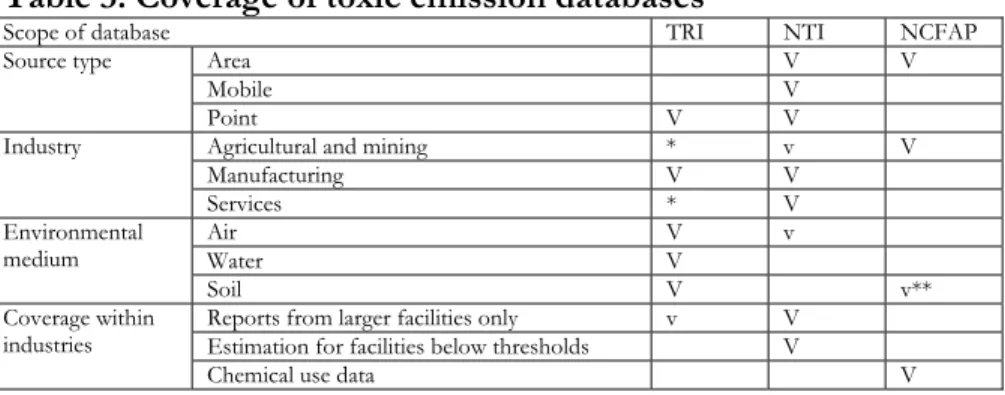
In CEDA, attention has been focused on solid coverage of emission sources rather than on inclusion of additional toxic pollutants. Table 3 summarizes the scope of the three databases in terms of emission source types, industries, environmental media and emissions from facilities below the threshold limit.

Table 3. Coverage of toxic emission databases

Scope of database TRI NTI NCFAP

Area V V

Mobile V

Source type

Point V V

Agricultural and mining * v V

Manufacturing V V Industry Services * V Air V v Water V Environmental medium Soil V v**

Reports from larger facilities only v V Estimation for facilities below thresholds V Coverage within

industries

Chemical use data V

* Since 1998 some of these activities have been covered by TRI.

** Whether the pesticide applied is an emission to air, water or soil depends very much on the properties of the applied chemical, climate conditions, etc. However, here the arguments are postponed to the stage of impact assessment method specification, and the emission itself is regarded as an emission to soil.

(25)

User’s guide

A glance at table 3 indicates that none of the databases cover emissions to water and land (other than pesticides) by mobile and area sources, NTI covering only Hazardous Air Pollutants (HAPs) and TRI mainly point sources only. While toxic pollutant emissions to environmental media other than air by mobile sources are not considered to be significant, those from area sources, such as leachate emissions from landfills, could be considerable. These gaps have meanwhile been fairly well filled, however, following a recent extension of the TRI databases, especially for Mining (SIC1021 to SIC1474), Logistic services (SIC4212 to SIC4581), Sewerage and refuse systems (SIC4952 and SIC4953) and Solid waste management (SIC 9511). In addition to these sectors, since 1998 most major chemical-handling sectors have also been included in the TRI database, and industry coverage by this database therefore seems reasonably complete, although obviously not 100 per cent.

E le c tr ic ity , S e we r a g e a n d r e fu s e s y s te m 3 6 % M in in g 1 % M a n u fa c tu r in g 6 1 % O th e r s 2 %

Total 3,669,196 ton of HAPs emission

Figure 2. Contribution by industries to NTI database by mass

This has indeed been confirmed, for air emissions at least. According to the NTI database, a total of 3,669,196 tons of HAPs was emitted in the US in 1996, with Manufacturing industries (SIC 20 – SIC 39) and Electricity, sewerage and refuse systems (SIC 49) contributing around 97%, emitting 2,202,304 ton and 1,338,170 ton, respectively. Thus, the major industries generating all but two per cent of HAP emissions are within the scope of the extended TRI database.

However, emission reports for the TRI database are collected only from those facilities employing 10 or more full-time equivalent employees or manufacturing or processing over 25,000 pounds or otherwise using over 10,000 pounds of any listed chemical during the reporting year. Although the emission from each individual facility not meeting these conditions may well be small, together they may be quite substantial.

The completeness of the TRI database has been examined using the NTI database and establishment size distribution data compiled by the Bureau of Census (2001). The NTI

(26)

database estimates HAP emissions using reports as well as emission factors and activity rates, regardless of the size of facilities. A comparison between TRI and NTI for overlapping chemicals can therefore provide an indication of the truncation of TRI of facilities below the threshold. This comparison showed that there are indeed significant systematic truncations in TRI showing only 17.2% of HAP emissions, on average, compared to NTI. This strongly suggests that using only TRI may significantly underestimate the potential impacts of toxic

releases.8_{One explanation might lie in the size distribution of establishments. Given the wide}

range of processes involved, each industry has different establishment size distribution characteristics. For instance, North American Industry Classification System (NAICS) 323, Printing and related support activities is dominated by establishments with less than 10 employees, which account for 66% of the total of 42,863 establishments, while the share of these smaller establishments in the Paper manufacturing sector (NAICS 322) is only 20% of the total of 5,868 (US Census Bureau, 2001). The larger the number of smaller establishments in an industry, the less complete the TRI data for that sector will probably be. Besides following from the nature of the threshold, this is also due to emission standards generally being less strict for small-sized establishments and again, although such establishments may

generate smaller volumes of toxic emissions individually, their sum total may be substantial.9

The regression study was further extended to the level of individual industries in order to reflect the differences in establishment size distribution. The TRI values for each sector represent, on average, 4.4% to 29.4% of the HAPs reported by NTI, depending on the sector

involved.10_{These results do not support the argument that TRI can still indicate the relative}

magnitude of toxic impacts even though their absolute values are misleading due to homogeneous truncation.

In CEDA 3.0, relatively complete data sources such as NTI for HAPs have been utilized as far as available. Otherwise, sectoral toxic emissions have been estimated based on TRI and the relationships between TRI and NTI values derived for each individual sector. In cases where no such sectoral relationships could not be established, owing either to sample size or to poor regression results, more general relationships between TRI and NTI have been used instead. For mobile and area sources, direct use has been made of the NTI database, with no further adjustments as it is considered to cover most major emissions. Besides point source emissions, the NTI database also includes emissions from natural processes and post-production stages, including wildfire, household product usage, etc., and these emissions have been excluded from subsequent assignment to individual industries.

8_{These results also support, to some extent, the study by Ayres and Ayres (1998).}

9_{Using the Bureau of Census (2001) data, the relationship between the completeness of TRI and the proportion} of small-to-medium sized establishments in each industry was examined. The results show that the two are negatively correlated.

10_{The coefficients of regression lie between 2.1 to 7.1, depending on the sector. Several significant differences} between TRI 98 (i.e. for 1998) and NTI for 1996 are observed for SIC 49, Utilities, although there was relatively little change in technology or regulation between the two periods. Formaldehyde and chlorine emissions, for instance, are reported to be 57.7 and 23.0 ton, respectively, by TRI98, while NTI for 1996 reports, for the same chemicals, 15,965.5 and 1,514.0 ton, respectively.

(27)

User’s guide

For pesticide emissions, direct use has been made of the NCFAP database. This database compiles and maintains volume records of 235 pesticides applied to 88 types of crop. On the assumption that the amount of pesticide applied equals emission, pesticide emission data have been assigned directly to a BEA industry code based on crop type.

3.2.5. Land use

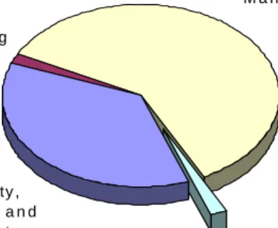
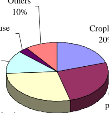
In this part of the CEDA database, only uses of land by major land-covering activities are accounted for (in square meters). In addition, mere occupation of land is all that is considered, with differences in neither land-use intensity nor land transformation being accounted for. Figure 2 shows the major forms of land use in the U.S.

Cropland 20% Grassland pasture and range 26% Forest-use land 28% Special uses 13% Urban use 3% Others 10%

Figure 3. Major uses of land in the US (USDA, 2002)

: Total area of land in use: 2.3billion acres (1997).

The Special uses cited in figure 3 include parks, wilderness, wildlife and related uses, transportation and national defense areas, while Others covers deserts, wetlands and barren land. Land uses that can be related to industrial production are croplands, grassland, part of Special uses (recreation, transportation and defense) and part of Urban use (for industrial installations). Urban use here includes industrial complexes and service areas other than agricultural uses, as well as urban residential areas. Most US industrial activities take place in urban areas, accounting for around 3% of land use in this category. The average land coverage of each BEA sector is thus less than 0.006% at most, and these figures have therefore not been

included in the CEDA database.11_{Among Special uses, natural parks are the largest category;}

11_{Furthermore, no statistics on land use were found that could be allocated to the detailed 6-digit BEA industry} level. As land use intensity in urban areas is considered relatively high, however, it is desirable to extend data coverage on Urban use further, especially as impact assessment methods that can properly account for land use intensity become available.

(28)

however, these are not considered to be an environmental intervention and have therefore not been included in the CEDA database either. The remaining industrial uses of land have all been allocated directly to BEA codes.

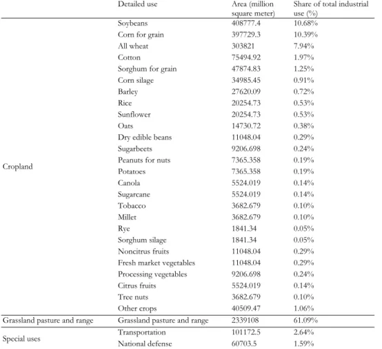
Table 4. Industrial uses of land in the US

Detailed use Area (million

square meter) Share of total industrial use (%)

Soybeans 408777.4 10.68%

Corn for grain 397729.3 10.39% All wheat 303821 7.94%

Cotton 75494.92 1.97%

Sorghum for grain 47874.83 1.25% Corn silage 34985.45 0.91%

Barley 27620.09 0.72%

Rice 20254.73 0.53%

Sunflower 20254.73 0.53%

Oats 14730.72 0.38%

Dry edible beans 11048.04 0.29%

Sugarbeets 9206.698 0.24%

Peanuts for nuts 7365.358 0.19%

Potatoes 7365.358 0.19% Canola 5524.019 0.14% Sugarcane 5524.019 0.14% Tobacco 3682.679 0.10% Millet 3682.679 0.10% Rye 1841.34 0.05% Sorghum silage 1841.34 0.05% Noncitrus fruits 11048.04 0.29% Fresh market vegetables 11048.04 0.29% Processing vegetables 9206.698 0.24% Citrus fruits 5524.019 0.14% Tree nuts 3682.679 0.10% Cropland

Other crops 40509.47 1.06% Grassland pasture and range Grassland pasture and range 2339108 61.09%

Transportation 101172.5 2.64% Special uses _{National defense} _60703.5 _1.59%

Land use data for the year 1998 were not available in the data sources considered, and 1997 data were used instead (USDA, 2002). According to trend analyses by USDA (2002), however, the pattern of land use for different activities has remained fairly stable and no readjustments were therefore made to estimate values for 1998. Several land use activities needed to be allocated to appropriate industries. As both industrial and household activities contribute to

land use for transportation, the share of the former was estimated based on the CO2 emissions

of passenger cars and other road vehicles such as trucks and buses. According to EPA (2002a)

passenger cars are responsible for 36% of total CO₂ emissions by road vehicles. Thus, only

(29)

User’s guide

on respective total production values.12_{Grassland pasture and range has been allocated to}

livestock industries, again based on total production value.

3.2.6. Nutrification

Nutrification is due principally to emissions of nitrogenous and phosphorus compounds to air, freshwater and soil. The main emission sources include combustion gases (for NOx to air) and application of fertilizer and manure (for emissions of nitrogenous and phosphorus compounds

to freshwater). NOx and NH3 emissions from these sources are fully accounted for in the

NET database. Although some nitrogenous emissions from manure application may subsequently undergo a series of biological processes known as nitrification and denitrification,

forming nitrite (NO2-), nitrate (NO3-) and nitrogen gas (N2), most are in the form of NH3 or

NH4+, depending on the ambient pH (or in the form of organic nitrogen), at the time of initial

manure application to agricultural soils. For nitrogenous emissions, direct use has therefore

been made of the NH3 inventory of the NET database

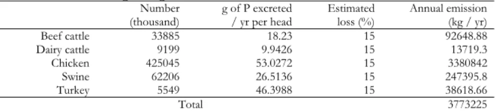
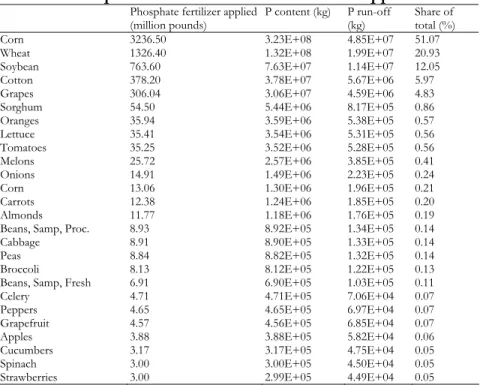
Emissions of phosphorus compounds are not readily available in any of the major statistical archives and these have therefore been estimated in terms of phosphorus equivalents, using a several databases. The CEDA inventory covers phosphorus emissions due to manure application and phosphorus run-off from phosphate fertilizer application.

Table 5. Major phosphorus emissions from livestock*

Number

(thousand) g of P excreted / yr per head Estimated loss (%) Annual emission (kg / yr) Beef cattle 33885 18.23 15 92648.88 Dairy cattle 9199 9.9426 15 13719.3 Chicken 425045 53.0272 15 3380842 Swine 62206 26.5136 15 247395.8 Turkey 5549 46.3988 15 38618.66 Total 3773225

* Own calculation based on Natural Resources Conservation Service (NRCS) (2000) and National Agricultural Statistics Service (NASS) (2003).

NRCS (2000) provides data on the average mass excreted daily by each type of livestock, its P content and the average run-off ratio. These data have been employed together with the NASS (2003) statistics on US 1998 livestock numbers to estimate annual P emissions to freshwater due to manure application.

Over half the phosphate fertilizer applied in the US is in the form of ammonium phosphate

(NH4HPO4), containing 88-90% of active ingredient. The phosphorus content of ammonium

phosphate fertilizer is thus around 22% by mass. NASS (1998, 1999, 2000, 2003) provides data on the amount of phosphate fertilizer applied to each type of crop (including fruits, vegetables and nuts). By applying the average phosphorus run-off rate to soil estimated by NRCS (2000), the level of phosphorus loss to soil was then estimated for use in CEDA 3.0.

12_{There are several “within-industry” uses of transportation that are not visible in the input-output table.} However, it has been assumed that utilization of transportation industry services reflects the relative magnitude of the transportation activities of each industry.

(30)

Table 6. Phosphorus emissions due to fertilizer application**

Phosphate fertilizer applied

(million pounds) P content (kg) P run-off (kg) Share of total (%)

Corn 3236.50 3.23E+08 4.85E+07 51.07 Wheat 1326.40 1.32E+08 1.99E+07 20.93 Soybean 763.60 7.63E+07 1.14E+07 12.05 Cotton 378.20 3.78E+07 5.67E+06 5.97 Grapes 306.04 3.06E+07 4.59E+06 4.83 Sorghum 54.50 5.44E+06 8.17E+05 0.86 Oranges 35.94 3.59E+06 5.38E+05 0.57 Lettuce 35.41 3.54E+06 5.31E+05 0.56 Tomatoes 35.25 3.52E+06 5.28E+05 0.56 Melons 25.72 2.57E+06 3.85E+05 0.41 Onions 14.91 1.49E+06 2.23E+05 0.24 Corn 13.06 1.30E+06 1.96E+05 0.21 Carrots 12.38 1.24E+06 1.85E+05 0.20 Almonds 11.77 1.18E+06 1.76E+05 0.19 Beans, Samp, Proc. 8.93 8.92E+05 1.34E+05 0.14

Cabbage 8.91 8.90E+05 1.33E+05 0.14 Peas 8.84 8.82E+05 1.32E+05 0.14 Broccoli 8.13 8.12E+05 1.22E+05 0.13 Beans, Samp, Fresh 6.91 6.90E+05 1.03E+05 0.11

Celery 4.71 4.71E+05 7.06E+04 0.07 Peppers 4.65 4.65E+05 6.97E+04 0.07 Grapefruit 4.57 4.56E+05 6.85E+04 0.07 Apples 3.88 3.88E+05 5.82E+04 0.06 Cucumbers 3.17 3.17E+05 4.75E+04 0.05 Spinach 3.00 3.00E+05 4.50E+04 0.05 Strawberries 3.00 2.99E+05 4.49E+04 0.05 ** Own calculation based on NASS (1998; 1999; 2000; 2003) and NRCS (2000).

3.2.7. Resource depletion

The only resources considered in CEDA are fossil fuels, iron ore, copper ore, and sand and gravel. Given the homogeneity assumption and the level of aggregation of the current IO table, there was felt to be little point in compiling data on other mineral resources. Thus, any purchase from the ‘inorganic chemicals’ sector, for instance, will be regarded by CEDA as a blend of all kinds of mineral resources from gold to silicon, regardless of the specific material actually purchased. Compared with other industries using natural resources, however, the energy sector and the iron and steel industry are reasonably homogeneous.

Figures for natural gas extraction have been taken from EIA (2003a), data on crude oil consumption from EIA (2000) and data on coal from EIA (2003b). Statistics for iron ore, copper ore and sand and gravel extraction are from USGS (2000).

(31)

User’s guide

4. Getting Started with CEDA 3.0

4.1. Starting CEDA 3.0 - Workspace

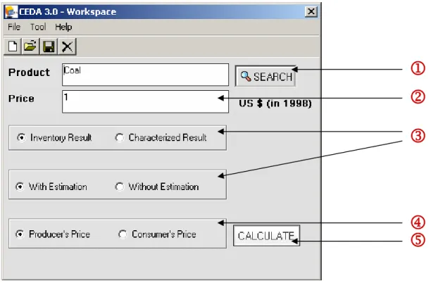
CEDA 3.0 is designed to accommodate an easy retrieval of the most detailed information that the CEDA 3.0 database contains. Starting up the program will open the window shown below.

1

2

3

4

5

Figure 4. CEDA 3.0 Workspace

Users need to select a commodity for which detailed environmental information is to be

retrieved. This is done by clicking the search button (1). Users can perform either keyword

(32)

7

6

8

Figure 5. CEDA 3.0 Search/Browsing window

Enter a keyword in the search window (6) and press enter or click search button (7), or

expand the folders shown in the lower half of the window to find the commodity that are to be selected by clicking relevant commodity categories. Then, press select (8). This will close the search/browsing window and activate the workspace again.

Type the price of the commodity selected in 1998 U.S. $ in the price window (2). Then, specify the types of information that you would like to retrieve by checking either of the two radio buttons located beneath the price window (3). The option ‘Inventory Result’ will retrieve information on individual environmental intervention and their amount generated to produce specified value of the commodity, and ‘Characterized Result’ will do it on environmental impact categories such as global warming, ozone layer depletion and toxic impacts. A detailed description on each individual characterization method used in CEDA

(33)

User’s guide

3.0 can be found in Guinée et al., (2002). CEDA 3.0 uses two sets of environmental intervention database: one with estimation and the other without estimation (see section 3.2.4. of this guide). Checking ‘With Estimation’ will use the environmental intervention database module that includes estimated toxic pollutants emissions in addition to self-reported data, where checking ‘Without Estimation’ will use the other one that is purely based on self-reporting.

Finally, users need to specify whether the price is in producer’s price or consumer’s price (4). When finished selecting all the options above, press ‘Calculate’ (5).

9

(34)

CEDA 3.0 provides two types of contribution analysis; output contribution and input contribution analysis (see section 2.3 of this guide). As the size of the results from such analyses is rather large (1334×480 or 86×480), visualizing the results is not very useful. Thus CEDA 3.0 facilitates export functions for further analyses using more sophisticated software tools such as Matlab and Mathematica. Users can chose either one of the two contribution analyses or the result appeared in the current window by checking one of the radio buttons shown at the bottom (9). Users can store the exported file either as a Microsoft Excel spreadsheet or as a text file (comma separated) ( ).

Figure 7. Message after a successful export (an example)