Institut für Visualisierung und Interaktive Systeme Abteilung Intelligente Systeme
Universität Stuttgart Universitätsstraße 38
D–70569 Stuttgart
Diplomarbeit Nr. 2973
Analysis and Visualization of
Coreference Features
Stefanie Wiltrud Kessler
Course of Study: Computer Science
Examiner: Prof. Dr. Gunther Heidemann Supervisor: Dipl.-Inf. Andre Burkovski
Commenced: October 15, 2009
Contents
1 Introduction 7
2 Coreference Resolution 9
2.1 Markables and Links . . . 10
2.2 Coreference versus Anaphora Resolution . . . 10
2.3 Applications for Coreference Resolution . . . 11
2.4 Why is it Hard . . . 12
2.5 Machine Learning for Coreference Resolution . . . 13
2.6 Visualization of Coreference . . . 14
3 Principal Component Analysis (PCA) 17 3.1 Graphical Explanation of PCA . . . 18
3.2 Computation of Principal Components . . . 19
4 Self Organizing Maps (SOMs) 23 4.1 Training of SOMs . . . 24
4.2 Visualization of SOMs . . . 25
5 The Project SÜKRE 29 5.1 Preprocessing . . . 30 5.2 Link Generation . . . 31 5.3 Feature Extraction . . . 32 5.4 Visualization . . . 32 5.5 Coreference Learner . . . 32 5.6 Database Design . . . 33
6 The Coalda Software 35 6.1 Requirements . . . 35 6.2 Conceptual Design . . . 37 6.3 Architectural Design . . . 39 6.3.1 I/O Libraries . . . 40 6.3.2 ActionLists . . . 40 6.3.3 UI Controls . . . 41
7 Features for Coreference Resolution 43
7.1 Markable Attributes and Link Features . . . 43
7.1.1 Content and Comparison Features . . . 44
7.1.2 Position and Distance Features . . . 45
7.1.3 Syntactic . . . 46
7.1.4 Grammatical . . . 47
7.1.5 Semantic . . . 48
7.1.6 Apposition . . . 49
7.2 Features Used by Ng and Cardie . . . 49
7.3 SÜKRE Feature Set . . . 51
8 Feature Analysis and Results 53 8.1 Exploration of the Feature Space . . . 54
8.2 Results of PCA . . . 56
8.2.1 PCA on the Ng Feature Vector Set . . . 56
8.2.2 PCA on the Filtered Ng Feature Vector Set . . . 59
8.2.3 PCA on the Filtered SÜKRE Feature Vector Set . . . 61
8.3 Visualization with Coalda . . . 63
8.3.1 Ng Feature Vector Set Visualized with Coalda . . . 63
8.3.2 Filtered Ng Feature Vector Set Visualized with Coalda . . . 65
8.3.3 Filtered SÜKRE Feature Vector Set Visualized with Coalda . . . 65
8.4 Evaluation of Visualization . . . 68
9 Conclusion 71
Bibliography 73
List of Figures
2.1 Example for Coreference (from the ARE Corpus) . . . 9
2.2 Basic Terminology . . . 10
2.3 Text-Based Visualization of Coreference . . . 14
2.4 Chain-Based Visualization of Coreference . . . 15
3.1 Example Data . . . 18
3.2 2D Scatterplot of Example Data . . . 18
3.3 Possible PCs for Example Data . . . 20
4.1 Different Visualizations of a SOM on Data with 6Variables, drawn with Matlab 26 4.2 U-Matrix, drawn with Matlab . . . 27
5.1 Modules in the SÜKRE Project . . . 29
5.2 Link Generation for Prelabeled Text . . . 31
5.3 ER-Diagram of SÜKRE Database Design . . . 33
6.1 Coalda GUI . . . 38
6.2 Architecture of the prefuse Visualization Framework [HCL05] . . . 39
8.1 Values for Feature PARANUM for the first250Feature Vectors . . . 54
8.2 Values for Feature WORD_OVERLAP . . . 55
8.3 PCA for Ng Feature Vector Set, plotted with The Unscrambler . . . 57
8.4 Scores for PC1for the first250Feature Vectors . . . 58
8.5 PCA for Filtered Ng Feature Vector Set, plotted with The Unscrambler . . . . 60
8.6 PCA for Filtered SÜKRE Feature Vector Set, plotted with The Unscrambler . 62 8.7 Ng Feature Vector Set Visualized with Coalda . . . 64
8.8 Filtered SÜKRE Feature Vector Set Visualized with Coalda . . . 66
List of Tables
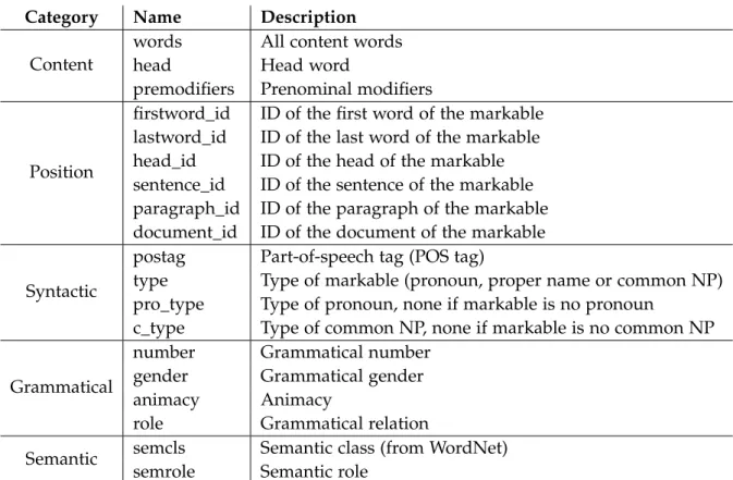
7.1 Attributes for Markables . . . 44
7.2 Features Used by Ng and Cardie [NC02] . . . 50
8.1 Comparison of Assignment and Gold Standard Label . . . 68
8.2 Evaluation Results . . . 69
Chapter 1
Introduction
When people talk about someone or something, they don’t always use the full name to refer to this person or thing. For example the personBill Clintoncould be referred to by part of his name likeClintonor a description likethe president or a personal pronoun likehe. All these expressions still refer to the same person. This is called coreference. A human listener performs coreference resolution intuitively to understand what the other person is talking about. We need computers to perform coreference resolution as well, in order to understand a text in natural language, because this is the natural way people talk and write.
There has been a lot of work on coreference resolution using rule-based systems or machine learning systems. But as the task is a difficult one, there are still a lot of unresolved problems. One of the issues in the development of machine learning systems for coreference resolution is the limited amount of training data available. For annotating a text with coreference, full understanding of the text and a basic level of linguistic knowledge is needed. This makes it more difficult to annotate a corpus with coreference information than with other linguistic information. One goal of the Coalda software presented in this work, is to facilitate the annotation of text with coreference information.
The second goal of the software is to enable a researcher to explore the space of the features used for machine learning. This should help the feature engineer to see areas in the data where coreferent data is not clearly separable from other data. With this information he might be able to design new features which better solve that specific problem.
In this work, a new visualization for coreference has been developed and implemented in a software called Coalda. This new visualization is not centered on the text, but tries to visualize the feature space. As it is impossible to directly visualize a high-dimensional feature space, an indirect way has to be found. In Coalda, the feature space is visualized by training a Self Organizing Map (SOM) and visualizing this SOM. The software allows the user to interactively explore the map, label feature vectors with coreference information and recalculate the map with different settings.
This diploma thesis is part of the DFG-project SÜKRE. The development of the mentioned interactive visualization is one of the main goals of the project. Other research topics are the development of new semantic and global features. Semantic features attempt to capture
1 Introduction
semantic information about the compatibility of the two markables that form the link. Global features are features that work on a partition of links that belong to one discourse entity. The remainder of this document is split into three main parts. First, the theoretical basis of this work is explained in the first three chapters.
Chapter2contains basic definitions for coreference resolution as well as a small overview of
the challenges of the problem, applications of coreference resolution and existing visualiza-tion approaches.
Chapter3 provides a very short explanation of the Principal Component Analysis (PCA).
The PCA is used later for the analysis of coreference feature vectors in chapter8.
Chapter 4 describes the training method for Self Organizing Maps (SOMs) along with
methods for the visualization of SOMs. A SOM is used in Coalda for the visualization of the feature space.
In the middle part, the implementation part of this thesis, Coalda and other modules in the SÜKRE project are presented.
Chapter5describes the context of this work as part of the DFG-project SÜKRE. The main
research topics of the project are presented along with a brief description of the software components that are used by the visualization software.
Chapter6contains details about the implementation of Coalda. This includes requirements,
a conceptual design and an overview of the architectural design.
Finally, in the third part, the developed feature sets are described and used in the evaluation of the new visualization.
Chapter7discusses different features for a machine learning coreference resolution system.
Two different feature sets are defined. These sets will be used for the evaluation.
Chapter 8contains the evaluation of the feature sets and the visualization. A PCA has been
applied to both sets to explore the structure of the data. The data has then been visualized with Coalda and the resulting visualizations are evaluated.
Throughout this document, code, shell commands and file system paths are written in
fixed font. Example sentences or expressions in natural language are written initalic.
Chapter 2
Coreference Resolution
Coreference resolution is an important task in natural language processing (NLP). Many applications rely on it to ”understand” a text written in natural language. Coreference is something widely used in natural language texts, but it is very hard for computers to understand. The definition is simple: if two expressions in a text refer to the same discourse entity, they are coreferent.
In some cases coreference is simple to determine. It is easy to detect that the expressions
(Jordan King Hussein)1and(Hussein)3in the example in figure 2.1are coreferent, because one
is a substring of the other. On the other hand intuitively two names that are not the same (likeHusseinandClinton) can never be coreferent.
For human readers the connection of(the president)4with the previously mentioned entity
(U.S. President Bill Clinton)2 is obvious. Although if expression2would only consist of(Bill Clinton)2we (as human readers) would need to know that he is (was) the president or the
text would need to contain that information somewhere.
To resolve a pronoun like(his)5we also need the context to decide whether it refers toHussein
orClinton.
The White House said on Monday(Jordan King Hussein)1would meet(U.S.
President Bill Clinton)2in Washington on April1and denied that the Middle
East peace process was unravelling.(Hussein)3 had been scheduled to meet(the
president)4on March18, but(his)5visit was postponed after a Jordanian soldier
shot dead seven Israeli girls near the Israel-Jordan border on March13and after
(Clinton)6had knee surgery on March14.
2 Coreference Resolution
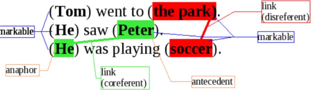
Figure2.2: Basic Terminology
2.1 Markables and Links
An expression that might be coreferent to another expression is called amarkable. The same thing is often called mention or coreference element in literature. All markables we are going to consider for coreference will be noun phrases. Anoun phraseis a group of words in a sentence that can be replaced by a (pro-)noun. For examplethe house ormy small yellow old house that my father built when I was a kid can be replaced by the pronounit.
Often a markable A is coreferent with another markable B and B is coreferent with yet another markable C. Such sets of markables that refer to the same entity are called coreference chains.
The opposite of coreferent is disreferent. Two expressions that do not refer to the same discourse entity, but to two distinct entities, are disreferent.
A pair of markables that can be co- or disreferent is called alink. This link has a number of associated link features. A link can have a label that contains information about co-/disreference of that link. The text in figure2.2has two labeled links.
The first markable in a link (in order of appearance in the text) is called antecedent, the second one is called anaphor. We assume that normally a link is created by linking a markable (the anaphor) with other markables which occurred earlier in the text.
2.2 Coreference versus Anaphora Resolution
Coreference resolution is closely related to anaphora resolution, but it is not the same. Anaphora resolution treats only expressions that depend on another expression for interpre-tation. The task is to find out what that other expression is. Anaphora is not a symmetric relation (for examplehemay depend onPeterfor interpretation, butPeterwill never depend on the pronounhe).
2.3 Applications for Coreference Resolution
The task of coreference resolution is to find expressions in the text that refer to the same discourse entity. This includes expressions that do not depend on other expressions for interpretation. Coreference is an equivalence relation, that means it is reflexive (every markable can be considered coreferent with itself), symmetric (ifherefers to the same entity asPeter, of coursePeterrefers to the same entity ashe) and transitive (ifheis coreferent with
the studentandthe studentis coreferent withPeter, alsoheandPeterare coreferent).
Not all coreferent links are anaphoras, for exampleQueen ElizabethandThe Queen Mother. Neither expression depends on the other for interpretation, so they are not anaphoric. But they refer to the same entity and therefore they are coreferent. Also coreference relations can occur across documents., but anaphora cannot.
But there are also anaphoric relations where anaphor and antecedent are not coreferent. For example in the two sentencesThe boy entered (the room). (The door) closed automatically. the expression The dooris an anaphor, because it depends onthe room for interpretation. But these two expressions are not coreferent, because they don’t refer to the same entity. More details on the distinction between anaphora and coreference resolution can be found in [Ng02] and [Ela05].
2.3 Applications for Coreference Resolution
When writing a text in natural language, we nearly always use different expressions to refer to the same entity. Also the expressions used to refer to an entity may contain new information about that entity. In order to still be able to get all the information about one entity and for general understanding of a text, we have to know which expressions refer to which entities. It is also important for some of the applications to consider cross-document coreference to collect information about an entity from different sources.
A selection of NLP tasks where coreference resolution is important follows, for more information and references see [Ng02].
Question Answering is the task of answering a question in natural language based on a corpus in natural language. We need coreference resolution to be able to connect a sentence likeHe was elected president in1993with the markable from the previous sentenceClintonin order to answer a question likeWho was president in1993.
The goal of Text Summarization is to produce a shorter version of a given text in natural language. This shorter version still has to contain the important facts about the main topic in the text. To solve that task, we need to know what the main topic of the text is. Typically this would be the entity most expressions in the text are coreferent with.
Information Extraction automatically extracts information from a given text in natural language and organizes it to machine readable structured information. To be able to add the information from different sentences to the correct entity and determine how many entities or events are talked about in a text we need coreference resolution.
2 Coreference Resolution
Machine Translation is the automatic translation from a text in one natural language to another natural language. Anaphora resolution is needed if there are differences in the language with regard to a feature of the antecedent. To be able to translate Das ist meine Brille, sie ist kaputtfrom German, whereBrilleis feminine and singular, to EnglishThese are my glasses, they are broken where glasses are neuter and plural, we need to know whatsie
refers to. The naive translation of siewithsheas inThese are my glasses, she is brokenwould not be understandable.
2.4 Why is it Hard
For coreference resolution many different sources of knowledge are needed. This ranges from morphological information like Part-Of-Speech tag (POS tag) to semantic information like semantic class. Every knowledge source has its level of correctness and may introduce wrong information. Some knowledge is very hard or expensive to compute (like semantical information) and has a high error level.
Even if some linguistic constraints indicate that two markables cannot corefer, sometimes they can. For example the assassination of her bodyguards (singular) can corefer withthese murders (plural) orDas Mädchen(the girl, neuter) withsie(she, feminine) [HKS09].
Often an expression refers to something that has been in focus for the last sentence. Tom went to the park. He saw Peter. He was playing soccer. In the second sentence there is a focus shift from TomtoPeter, so the pronounhein the last sentence probably refers toPeter(also because we have no information aboutTomplaying soccer earlier). But if the last sentence would beHe was happyit would not be obvious even to a human reader. Focus is hard to determine. Centering theory [Ela05, Ng02] tries to track entities in focus, but this is a very
hard problem in itself.
Sometimes a lot of world knowledge is required to correctly determine the antecedent of a noun phrase. For example (The boys) were kidnapped by (masked men). After (they)1blindfolded
... After (they)2 were released .... The first theyrefers to masked men, the second tothe boys.
This text is understandable for us humans only because we know that kidnappers blindfold their hostages while the hostages are the ones to be released [Ela05]. World knowledge is
very difficult to formalize and it is very hard to determine what exactly is the information we need. This is also the case when coreference depends on the time a text was written or similar information. WhetherObamaandthe president of the United Statescorefer, depends on the result of the election and the time the text was written.
Some categories of noun phrases are harder to resolve than others. Proper names are easiest because coreference can be very well recognized with string matching and alias matching. Common nouns are harder, especially definite noun phrases (for example the door orthe president). Not all definite noun phrases are anaphoric, some already uniquely identify an entity. That means the first problem is to determine the anaphoricity of a noun phrase. The distance from a definite noun phrase to its antecedent can be greater than the distance of a
2.5 Machine Learning for Coreference Resolution
pronoun to its antecedent. Definite noun phrases may also refer to entities not in focus while pronouns mostly do [Ela05, SGCR09].
Additionally, there are markables which are not coreferent with any other markable that has occurred in the text onto this point. These ”singletons” can be markables that are self-explaining or the only mention of an entity in the text. A second kind of singletons are markables that are the first mention of the entity in the text (if we consider only links of markables with markables that occurred earlier in the text). Adding anaphoricity determination to a system would help to save computation time, because for singletons no antecedents have to be searched. It would also prevent errors, because any antecedent to a non-anaphoric noun phrase is certainly wrong.
To determine anaphoricity of a noun phrase is a difficult problem. Ng and Cardie [NC02] use
a feature that indicates the anaphoricity of a markable. This feature is calculated by a separate anaphoricity classifier. On the other hand Luo [Luo07] argues, that the determination of
anaphoricity is a part of coreference resolution. He uses two models, where one determines the most probable antecedent for an anaphoric markable and the other determines whether a markable is a singleton.
In the training of classifiers for coreference it is important to keep in mind that coreference is a very rare relation. The vast majority of links are not coreferent. The MUC-6 corpus for
example contains only2% positive instances [Ng02].
2.5 Machine Learning for Coreference Resolution
Machine learning algorithms are often categorized in two basic categories, supervised learning and unsupervised learning. Supervised learning algorithms work on data that has been labeled with the class information. From this data the algorithm creates a classifier that can predict the class of a new input. Unsupervised learning works on unlabeled data and attempts to find structures that are inherent in the data itself.
Applying a supervised learning algorithm to the coreference resolution problem means to classify every link between two markables as coreferent or disreferent. Such a link-based classification system is the decision tree classifier used by Soon [SNL01] and later Ng and
Cardie [NC02].
But coreference resolution can also be viewed as a clustering task. Clustering is an unsuper-vised learning method. The inherent structure of the data that needs to be found is the group of markables that refer to each entity mentioned in the text. Cardie and Wagstaff [CW99]
cluster markables using a manually defined distance metric over a set of link features. For all of these machine learning algorithms a set of features is needed. The features are used to measure the similarity of the two markables forming a link or to calculate the probability that this link is coreferent. A subset of the feature set used by Ng [NC02] has
2 Coreference Resolution
The White House said on Monday(Jordan King Hussein)1would meet(U.S.
President Bill Clinton)2in Washington on April1and denied that the Middle
East peace process was unravelling. (Hussein)1had been scheduled to meet(the
president)2on March18, but(his)1visit was postponed after a Jordanian soldier
shot dead seven Israeli girls near the Israel-Jordan border on March13and after
(Clinton)2 had knee surgery on March14.
Figure2.3: Text-Based Visualization of Coreference
Coreference is a transitive relation. If a markable A is coreferent with B and B is coreferent with C, then A also has to be coreferent with C. Properties like this cannot be enforced by any system that works on links only. Other restrictions for a valid entity are for example that an entity cannot consist only of pronouns. Apart from not using links where both markables are pronouns (which creates other problems) such restrictions cannot be expressed only in link-features [HKS09].
To deal with such problems, recent systems for coreference resolution work on clusters, not links [CGB08]. This allows to formulate ”global” features that take all available information
about an entity into account.
The SÜKRE project uses a link classifier as well as a cluster-based classifier as described in section5.5.
2.6 Visualization of Coreference
There are different methods of visualization for coreference. Visualization can center on the text, on coreference chains or on the feature space.
The most intuitive visualization of coreference is text-based visualization. The text is shown, the markables are marked and a coreference chain is connected by lines (as in MMAX [MS01])
or the entity is identified with numbers (as in CorefDraw [HBTM01]) or colors (as in GATE
[CMBT02]). This does not show the features or the feature space and what links are similar
to others. It is also limited by the paper and the number of coreference lines/colors one can understand. This makes it difficult to analyze large chains or inter-document coreference or many links at ones.
Figure2.3contains the example sentence used earlier in this chapter visualized with
text-based visualization. Every markable is denoted by parenthesis, and the entity it is referring to is identified with a unique ID. The Coalda Software offers a simple text-based visualization for the feature vectors associated with one node of the SOM only, to make the text of the links available to the user.
A step in the direction of more abstract visualization is chain-based visualization. The chains from the example text are visualized in 2.4. Coreference chains are shown and the user can
click on the chains to see the markables that form the chain. This representation only serves
2.6 Visualization of Coreference
U.S. president Bill Clinton(NP:id2) 1
the president(NP:id4)
Clinton(NP:id6)
Jordan King Hussein(NP:id1) 2 Hussein(NP:id3)
his(NP:id5)
Figure2.4: Chain-Based Visualization of Coreference
to visualize and navigate the result space, not the feature space. Additionally, the markables are shown without context which makes it hard to judge if a link is correct or not.
Witte and Tang [WT07] use this kind of visualization in their graphical representation of
results obtained by a machine learning coreference resolution system. The visualization can be explored by users for browsing of recognized coreference chains and error detection and analysis. They represent coreference chains by Topic Maps and OWL Ontologies and use existing tools for the visualization of document navigation. For the error analysis a manually defined ontology is used. The extracted chains are compared to a gold standard and put in several classes in the ontology like ’correctChain’ or ’hasNPmissing’.
In feature space visualization the visualization does not center on the text, but on the feature space. As it is impossible to directly visualize a high-dimensional feature space, an indirect way has to be found. In the Coalda software the feature space is visualized by training a SOM and visualizing this SOM (see chapter6).
Chapter 3
Principal Component Analysis (PCA)
In this chapter a very short explanation of the Principal Components Analysis is given. The PCA is used for the analysis of coreference feature vectors in chapter8.
The idea of PCA is to reduce the dimensionality of a data set and at the same time keep most of the information that is in the set. To achieve this, the original variables are transformed into a new coordinate system that is spanned by so-called principle components (PCs). The PCs can be thought of as ”hidden variables” that cannot be directly observed, but are responsible for the structure of the data. The number of PCs that are needed to explain the structure of the data is smaller than the number of variables in the original data set.
These PCs are ordered by the amount of variation of the data they explain. All PCs are uncorrelated with each other, unlike the original dimensions. Geometrically the first PC can be thought of as the vector on which the projection of the data causes smallest loss of information (smallest sum squared error). After the projection on this axis, the data has maximum variation. The second PC has the second-smallest loss of information while being orthogonal to the first PC and so on.
The data can be plotted in the new coordinate system of the first two or three PCs. It is now easier for humans to see the inherent structure of the data and find clusters or anomalies. Additionally, correlations between variables can be found. The PCA will also show which variables are important for the model.
The PCA was first introduced by Karl Pearson in1901. In1933it was re-invented by Harold
Hotelling. But the method became widely known (and used) only when computers allowed the computation of principle components without a lot of effort. It is today often used as a tool in exploratory data analysis in many areas.
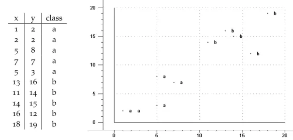
3 Principal Component Analysis (PCA) x y class 1 2 a 2 2 a 5 8 a 7 7 a 5 3 a 13 16 b 11 14 b 14 15 b 16 12 b 18 19 b
Figure3.1: Example Data Figure3.2:2D Scatterplot of Example Data
3.1 Graphical Explanation of PCA
To show with an example1what the PCA can do, we take the data in table3.1. This data is
only two-dimensional, so we are able to plot even the original data. In the plot in figure3.2
we see that the data forms two clusters, the two classes that are labeled witha andb. The PCA tries to draw a line through the data so that the difference between the clusters becomes apparent. The best line to achieve this is a line, where the distance from each data point to the line is minimal. This distance is the information we lose when we use the projection on the line as the only information.
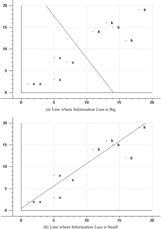
If we draw a line just at random, as for example the line in3.3(a), it doesn’t give the desired
result. The projections of all data points are very close together and we cannot see the two clusters we expect to see. The sum of all distances from all points to this line is big, this means that a lot of information is lost.
The line in3.3(b) fits the data much better than the first line. It does minimize the distance
from all points. It also maximizes the variation in the data, the data points are far away from each other and we can clearly distinguish the two clusters. This line is the first principal component of the data. We have reduced the dimensionality of the original data set from two dimensions to one and still kept most of the information. The information we have lost is not relevant for us in understanding the structure of the data.
To find a second principal component, we have to find a line orthogonal to the first one. In case of the example data, there is only one possibility. If we had a data set with more dimensions, we would again have to choose a line orthogonal to the first line, that maximizes variation and minimizes the information loss.
1
This example can be found in more detail in [Kes07]
3.2 Computation of Principal Components
The coordinates of the original data can now be transformed to the new coordinate system and the data can be plotted in this new coordinate system.
3.2 Computation of Principal Components
Mathematically doing a PCA corresponds to finding the eigenvectors of the covariance matrix of the data. The first PC is the eigenvector with the largest eigenvalue, the second PC with the second largest and so on.
Before doing a PCA the data has to be centered. To center the data, the mean of the variable is subtracted from every variable. The meanµX of the variableXwhere the sampleihas the
valueXi is defined as
µX= ∑ n i=1Xi
n
and denotes the ”middle point” of the data set.
The next step is to calculate the covariance matrix of the data. The variance var(X)is a measure of the spread of data in a variable. It is the mean ”distance” (deviation) of the samples fromµX. The formula is for discrete samples
var(X) = ∑
n
i=1(Xi−µX)2 n
Mean and variance are one-dimensional. To find out how much two variables change with respect to each other, the covariance of these two variables can be calculated. The covariance of a variable with itself is always its variance. If the covariance is positive, the variables are correlated and increase together. If the covariance is negative, the variables are negatively correlated, if one variable decreases the other one increases. If the covariance is zero, the variables are independent of each other. The formula for calculating the covariance of variablesXandY is
covar(X,Y) = ∑
n
i=1(Xi−µX)(Yi−µY) n
The covariances between all variables are often displayed in a matrix, this is called the covariance matrix. The covariance matrix is a square and symmetric matrix.
Once the covariance matrix of the data set is calculated, we have to find the eigenvectors of this covariance matrix. A vector is an eigenvector of a given matrix, if the multiplication of the vector with the matrix results in an integer multiple of the original vector. This means that the vector does not change its direction in the vector space, only its magnitude. Eigenvectors can only be found for square matrices. All eigenvectors are orthogonal to each other. Often eigenvectors are normalized to have a length of one.
Every eigenvector has a corresponding eigenvalue. This is the amount by which the original eigenvector is scaled by the multiplication with the matrix.
3 Principal Component Analysis (PCA)
(a) Line where Information Loss is Big
(b) Line where Information Loss is Small
Figure3.3: Possible PCs for Example Data
3.2 Computation of Principal Components
Mathematically this means a vector~v is an eigenvector of matrixAif
A~v =λ~v
whereλis the eigenvalue corresponding to~v.
The calculation of eigenvectors is done by numerical methods. The valuesvi of the
eigenvec-tor~vin the original dimensions are called loadings.
The eigenvectors are then ordered by their eigenvalues. The eigenvector with the biggest eigenvalue is the first principal component, the one with the second biggest eigenvalue the second principal component and so on.
Finally, we only need to convert the coordinates of the data in the original space to coordinates in the new eigenvector space. To do this, we put the eigenvectors we want to use in the eigenvector matrix. In this matrix, the eigenvectors are the columns. The first column contains the eigenvector with the biggest eigenvalue, the last column the one with the smallest eigenvalue.
We map the data points onto the eigenvectors by multiplying the transpose of the eigenvector matrix with the data matrix. The data in the new coordinate system can then be plotted. The values of the data points in every PC are called scores.
To summarize, to do a PCA for the data matrixDwith poriginal variables we have to
1. Calculate the mean for each of the poriginal variables and center the data. 2. Calculate the covariance matrix for all original variables.
3. Find the eigenvectors of the covariance matrix.
4. Sort the eigenvectors by their eigenvalues and selectk peigenvectors we want to
use for display.
5. Calculate the new coordinates of the data points in the eigenvector space. 6. Plot the data in the new coordinate system.
Mathematical proofs of the properties of PCA can be found in [Jol02]. For more practical
Chapter 4
Self Organizing Maps (SOMs)
This chapter will introduce Self Organizing Maps which are used in this work for the visualization of coreference links, as explained in chapter6.
A Self Organizing Map (SOM) is a neural network (non-linear unsupervised learning algorithm) first described by Teuvo Kohonen in1982[Koh82]. It is a method to map a high
dimensional feature spaceRin onto a low dimensional output spaceRout(for visualization typically three dimensions or less). A SOM preserves the topological properties of the feature space, so that feature vectors that are close together in the input feature space will be close together as well in the output space.
Motivation for this type of neural networks comes from the human brain, where the information from neighbouring visual inputs is processed by neighbouring regions in the visual cortex [Roj96].
A SOM consists of a grid of map units (also called nodes or neurons). This grid has the dimension of the output spaceRout. For a two-dimensional output space the grid is usually hexagonal or rectangular. Every node has a fixed place on this grid and fixed neighbours. These neighbourhood relations are never changed.
Additionally every node has a weight vector of the same dimension as the input data vectors (Rin). These weight vectors are adapted in training so that the nodes of the SOM change
their place in the feature space to get closer to the data points. Also the weight vectors of the neighbouring nodes are adjusted, so that nodes near to each other on the grid are also near to each other in the feature space.
Because the nodes change their places in feature space to get closer to the data points, at the end of training most nodes will be in areas where there are many data points. Only a few nodes will be in areas where there are few data points. This means, not only the topology of the data is approximated by the SOM, but also the data density distribution.
4 Self Organizing Maps (SOMs)
4.1 Training of SOMs
For the training algorithm of SOMs, two functions that monotonically decrease with training time t are required. One is the learning coefficient α(t), the other is the neighbourhood
function hij(t)which describes the neighbourhood of node j. Neighbourhood is defined on
the neighbourhood relations of the lattice. Both, learning coefficient and neighbourhood function, get smaller with training time.
A typical choice for the neighbourhood function ishij(t) =exp(−
||w~i−w~j||2
2σ(t)2 )whereσ(t)is the
radius of the neighbourhood and decreases with time (Gaussian function).
The learning coefficientα(t)controls how much the current input influences the training. At
the beginning of the training it is big. Then it decreases with time.
We also need a distance metric for the feature space Rin. This is usually the euclidean distance, but could be any distance metric.
At the beginning of the training, all weight vectors are initialized. If there is no prior knowledge about the data, the weights are initialized at random.
The training algorithm of a SOM has the following steps:
1. Chose a random input vector~x(with dimension of the feature spaceRin) from the data
points.
2. The input~x is given to all nodes of the SOM. Calculate the distanced(w~i,~x) for all
nodesiand take the nodekwith the minimum distance (the node nearest to~x). It is called Best Matching Unit (BMU).
3. Update all nodes, the update formula for a neuroniwith weight vectorw~
i is ~
wi(t+1) =w~i(t) +hik(t)α(t)(~x−w~i(t))
wherekis the BMU. This means, that the nodek is now pulled in the direction of the input~x. The neighbours are also pulled in that direction. Nodes nearer to the BMU are adapted more than nodes further away in the neighbourhood. Weight vectors of nodes outside the neighbourhood are not changed at all.
4. Increaset(which decreasesα(t)andhij(t)).
5. Repeat for a new input vector until limit of iterations is reached or otherα(t)is smaller
than a specified threshold value.
At the beginning of training, when α(t) and hij(t) are still big, the net is only roughly
adjusted to the data. Once the values get smaller, the weight vectors of single nodes are fine tuned.
Training can also be done in batch mode, where the whole data set is presented to the net before any adjustments are made. The new weight vector of a node is then calculated with the adjustments that would have been made for all the nodes that have this node as a BMU
4.2 Visualization of SOMs
[VHAP00]. The advantage of this processing is, that it is deterministic. For the same data set
the resulting map is always the same. This makes the result of the training reproducible. A lot of literature on SOMs exists. For a short explanation with some examples for the appli-cation of SOMs consult [ZG93] or [Imo08]. For a more in depth discussion use [RMS90].
4.2 Visualization of SOMs
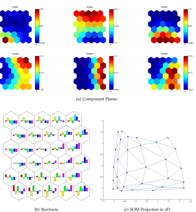
Visualizing the SOM in output space is easy. The output space has a small dimension and the neighbourhood relations are fixed. The result would be a grid and every map with the same topology looks the same. But what we want to visualize is the feature space as represented by the SOM. This feature space is still high dimensional, and so it is hard to visualize. The easiest way of visualizing the feature space is to show the weight values of the SOM map units in every dimension in feature space on component planes (see figure4.1(a) on
the next page). For a limited number of dimensions it is also possible to show the different values in these dimensions in one map unit with barchars or other statistics (see figure4.1(b)
on the following page). In the same way one can use colors or numbers to visualize the number of feature vectors having one map unit as BMU.
One can also visualize the similarity of nodes to each other by coloring [Ves99]. Similar
nodes get similar colors. If done in a single dimension this gives the component plane. For two or three dimensions one can take the dimensions as two/three dimensions of the RGB-space. For more than three dimensions the weight vectors need to be projected on the RGB-space.
SOMs can also be visualized by a projection in2D or3D. The two or three dimensions to be
shown can be dimensions of the feature space or the first two/three principal components. An example of a projection in2D is shown in figure4.1(c) on the next page.
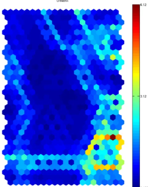
The most common visualization for SOMs is the U-matrix (unified distance matrix) [US90].
The U-matrix displays the distance of a node to its neighbour nodes. To prevent the vector distance from being influenced by a dimension with high values, the values of all dimensions should be normalized.
The U-matrix is shown in a grid with the same topology as the map. If the map is hexagonal, the U-matrix will contain hexagonal cells. There is one cell for every node at the place that node has in the input space. Additionally for every edge between two neighbouring nodes there is a cell at the location of the edge. In a hexagonal grid a cell for a node i will be surrounded by six cells for the edges.
For every cell the U-matrix value is calculated. The U-matrix value for an edge is the distance in feature space of the two nodes of that edge. Any distance metric may be chosen, normally the Euclidean distance is used. The U-matrix value of a node can be set arbitrarily, but is normally set on the mean value of all edges from this node. The result is an overview of the distance structure of the map in feature space.
4 Self Organizing Maps (SOMs)
(a) Component Planes
(b) Barcharts (c) SOM Projection in2D
Figure4.1: Different Visualizations of a SOM on Data with6Variables, drawn with Matlab
4.2 Visualization of SOMs
Figure4.2: U-Matrix, drawn with Matlab
The U-matrix value of a cell is visualized with different colors. Figure4.2shows an U-matrix
as generated by Matlab. Blue color means low U-matrix value, red color means high U-matrix value.
So the blue areas are nodes that are close together, that means they form a cluster. Nodes with a high U-matrix value (red) are very far away from their neighbouring nodes, the long (red) edges are the cluster boundaries. As the SOM preserves the topological properties of the original data, this means that there is also a cluster respectively cluster boundary in the original feature space.
In the U-matrix it is impossible to see how many feature vectors are near a specific node or how close the feature vectors are. The P-matrix [Ult03a] shows the density of the data
around the nodes. It can be any density estimation, normally the Pareto Density Estimation (PDE) is used. The PDE calculates the number of feature vectors in a hypersphere (Pareto sphere) around a node. At every node the density of data around this node is displayed in the P-matrix. Neurons with a large P-matrix value are located in regions of the feature space with high density, nodes with small P-value are in regions with few data points. The P-matrix visualizes the data density structure of the data.
It is possible to combine U-matrix and P-matrix in the U*-matrix [Ult03b]. The idea is that
in areas with high data density the distances between nodes should be valued less than in areas with low density, where they are always cluster boundaries. The U*-matrix value for edges is the same as the U-matrix value. The U*-matrix valueU∗(n)for the noden is
U∗(n) =U(n)· P(n)−mean(P)
mean(P)−max(P), whereU(n)is the U-matrix value, P(n)is the P-matrix value
Chapter 5
The Project SÜKRE
The project ”SÜKRE” is a project funded by the Deutsche Forschungsgemeinschaft (Ger-man Research Foundation). ”SÜKRE” stands for ”SemiüberwachteKoreferenzErkennung” (”semi-supervised coreference resolution”). The participants are the Institute for Natural Language Processing and the Institute for Visualization and Interactive Systems of the University of Stuttgart. The project has started in September2009and will go on for two
years. This diploma thesis is a part of the SÜKRE project.
The goals of the project are detailed in [HKS09]. One main topic is the development of an
interactive visualization for coreference features. This visualization should facilitate the semi-supervised annotation of large amounts of training data. This training data can then be used to explore new features. Features that will be explored in the course of the project are semantic features and global features. Semantic features attempt to capture semantic information about the compatibility of the two markables that form the link (see section
7.1.5). Global features are features that work on a partition of links that belong to one
discourse entity.
As the topic of this work is in the visualization of link features, this chapter will only give an overview about the part of the project that deals with link features. It will not talk about the global features although they are a big research topic of the project. But a visualization similar to the one developed here could be used for visualization of global features.
5 The Project SÜKRE
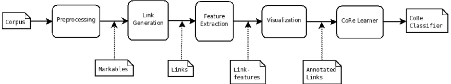
In figure5.1on the previous page you see on overview about the modules in the project.
Every module takes as its input the information generated by the preceding modules. The preprocessing, link generation and the CoRe Learner module are developed in the Institute for Natural Language Processing. The visualization module is work of the Institute for Visualization and Interactive Systems. The feature extraction for link features is work of both institutes in cooperation.
In the following each module is described in more detail. At the end, in section 5.6, the
design of the database which is used by all modules is described.
5.1 Preprocessing
The preprocessing is different for prelabeled and unlabeled text. Goal of the project is to work on unlabeled text that is to be labeled with the help of the visualization. For the start of the project and the first analysis, labeled text has been used (namely the corpora of ARE, ACE2005and MUC-6).
For prelabeled text the words and labeled markables are extracted from the text and also all the word and markable features that are available. For the MUC-6corpus this is POS-tag and
number. All other markable features are extracted as they would be from unlabeled text. Coreference information in the MUC-6corpus is labeled in the form of coreference chains.
The markables are extracted from these chains. So only markables that are coreferent with something are extracted. So a lot of noun phrases that would be markables if we processed the unlabeled text are not considered at all.
For unlabeled text more preprocessing is needed. After tokenization, sentence boundary detection and POS tagging, markables need to be extracted. As we consider only noun phrases as markables and every noun phrase could be a markable, the easiest way to do this will be to use the output generated by a parser. A parser will also provide POS-tags. The preprocessing for unlabeled text is currently in development.
At the end of this step all the information about the corpus is contained in four tables of the database. The first table contains all sentences from all documents (table ”sentences”). In an other table every word from every sentence is saved along with its features (table ”words”).
The markables that are extracted from the text are saved (table ”markables”) along with a potential entity that could be contained in that markable (table ”entities”). These entities are only based on noun clusters and proper names found in the markables.
5.2 Link Generation
Coreferent links: A m1 B m2 m3 C D
Disreferent links: A m1 B m2 m3 C D
Figure5.2: Link Generation for Prelabeled Text
5.2 Link Generation
After the markables have been extracted, they have to be put together to be pairs of markables (links). The link generation for prelabeled text is visualized in figure5.2.
For prelabeled text, the markables of a conference chain are linked to create positive training samples. For a chain containing the markables A, B, C, D (in order of appearance in the text) the following links will be created. First A is linked with all other markables of the chain, creating the links A-B, A-C and A-D. The same is then done for B and the rest of the markables.
To create negative training examples, every markable of a chain is paired with markables of other chains that come close after them in the text. The generation is stopped as soon as the same number of disreferent links has been created that there are coreferent links from that markable. At the moment no links of markables in different documents are created.
In this step also a filtering process is done to reduce the number of links presented to the user. Filters can be defined by the user. The idea is that links that are certainly disreferent are filtered out. This could include for example links where one markable spans the other or links where a reflexive pronoun is linked with a markable from a different sentence. The filter can also be used to limit the links down to a certain category. It might be useful to limit the distance of the two markables that can form a link or to consider only coreference inside one document. After a first step where these links are labeled, more links could be included in a second labeling step.
The result is the link table that contains the two markables that form the link and a label for that link. For labeled data the label is taken of the gold standard provided by the corpus. The confidence value of this label will always be 100. For unlabeled data the label will
initially be set to unknown. At this point some prelabeling could be introduced where some ’very probably coreferent’ links could be marked. This could be links where there is an exact string match of the markables or other heuristics. This label would help in labeling by giving the user some starting points to check.
5 The Project SÜKRE
5.3 Feature Extraction
For every link, a set of features is computed based on the attributes of the markables and words and other knowledge sources. The link features are not added to the link table, but they are kept in a separate feature vector table. This is because a link can have various feature vectors with different features calculated on this link.
This module is developed by both institutes in cooperation. At the moment it consists of two components, one developed in the Institute for Natural Language Processing, the other in the Institute for Visualization and Interactive Systems.
The first component calculates basic features like String match, edit distance or agreement on grammatical attributes. Features can be defined with the help of regular expressions. The second component calculates a set of features that cannot be defined by regular ex-pressions. These include for example the features for acronyms, apposition or non-linear features.
The feature extraction module is very modular so that new ideas for features can be tested easily. This is especially relevant for the semantic features to be developed in the project. A parser is already used for semantic role labeling and tests on parse tree features. WordNet is used for information about semantic class. Other sources for new features could be search engine distance or Wikipedia.
5.4 Visualization
The visualization takes the feature vectors from the database, maps them to a SOM and displays the SOM to the user. The user interactively explores and labels the data. The labels are added to the link table in the database. It is possible for the user to select a subset of the feature vectors to visualize and to recalculate the SOM for this subset. Also the user can chose the features he wants to use for the visualization.
Calculations are saved in the calculations table of the database.
This module is described in more detail in the next chapter, chapter6on page35.
5.5 Coreference Learner
The data labeled with the visualization module can now be used to train a link-based classifier for coreference resolution. As feature set the same features can be used as for visualization or different features. This is because some features might be useful for visualization but not for training and vice versa.
At the moment the implemented machine learning algorithms are Support Vector Machine, a Naive Bayes Classifier and Regression (Ordinary Least Squares).
5.6 Database Design
Figure5.3: ER-Diagram of SÜKRE Database Design
5.6 Database Design
All modules of the software operate on a common database. This database is implemented as a Postgres database for the modules developed in the Institute for Visualization and Interactive Systems. The other components use the same design, but work on files.
5 The Project SÜKRE
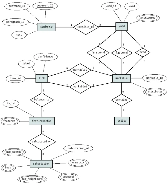
An ER-diagram of the design of the database is shown in figure5.3on the previous page.
Thesentencetable contains all sentences from all documents in the corpus with document ID, paragraph ID, sentence ID and the content of the sentence.
Sentences consist of a number of words. The word table contains all words from all documents of the corpus. For every word it contains the word itself as text, a unique word ID, the document ID, paragraph ID, sentence ID and a list of attributes. The attributes can be any kind of linguistic information like POS tag, number, gender or semantic class. The attributes are saved as an array, not in separate columns to keep the design flexible for changes in the number and type of attributes. Punctuation marks also count as words. Themarkabletable contains all the markables of all documents. They also have a unique ID. The words the markable consists of are contained indirectly as references to the first and the last word of the markable. Also the ID of the head is saved. As the words are numbered in order of the text, the ID of the last word in a markable has to be bigger than the ID of the first word and the head has to be somewhere in between.
Markables also have a list of attributes such as number, gender, etc. Often the markable attributes will just reflect the attributes of the head. But sometimes the markable attributes can differ from that, for example a markable could be plural even if the head is singular (the markablea cat and a dogwould have the singular wordcatas a head after our preprocessing, but the grammatical number of the markable in total is plural).
The markable table contains a reference to a potential entity that could be contained in the markable. Thisentitytable contains a first approximation of entities that could be found in the text with the word IDs of their start and end word.
A word can be part of multiple markables if the markables overlap. This should only be the case if one markable is embedded in the other one. This is the case for example in the markable(the president of (America)2 )1.
A link is always formed by two markables. Supposedly the same link is only generated once. A markable can be part of any number of links. Thelinktable contains a unique link ID for every link, a reference to the two markables that form the link and a label (coreferent or disreferent or unknown) and the confidence value (between0and100) of that label.
For one link any number of feature vectors can be generated. It would make sense to calculate different feature vectors with different sets of used features. The resultingfeature vectortable contains a unique feature vector ID, the ID of the link the features belong to and a list of features.
Finally the calculation table contains the SOMs calculated for the visualization. Every calculation has a unique ID. A number of vectors and matrices with information about the SOM is stored along with the IDs of the feature vectors that have been used as input in this calculation.
Chapter 6
The Coalda Software
The new visualization that has been developed in this work is implemented in the Coalda software. Coalda stands for Coreference Annotation of Large Datasets. This chapter contains the specification of requirements for the visualization software, a conceptual design of the visualization and a high-level architectural design.
The conceptual design is the first design of the software intended for the user, not the programmer. It describes the functions and the basic structure of the software. It leaves open how the single functions are to be implemented. In contrast, the architectural design is directed at the programmer and already contains some information about the structure of the modules and the technology used.
6.1 Requirements
Requirements are listed in categories following the the VAI standard of documentation [Car06]. The following categories are used:
RF Functional requirements list the functions the system has to execute (”what” does the system do).
RU User requirements list the desired options for the user interface (”how to access” what the system does).
RP Performance requirements denote minimum requirements in terms of time and space (”how fast”). These are always measurable.
RO Operational requirements define file formats, operating systems and other resources that are to be used.
Requirements are marked as ”essential” if they are a crucial part of the system, ”desirable” if they would add a considerable enhancement to the system and are considered important and ”optional” if their realization would add functionality to the system that is merely nice to have.
6 The Coalda Software
Functional Requirements
RF1 The input data to be visualized are feature vectors belonging to links (pairs of markables) [essential]
RF2 The feature space is visualized using a SOM [essential]
RF3 The structure of the SOM is visualized using the U-matrix [essential]
RF4 The number of feature vectors associated with a node is shown by colors or labels [desirable]
RF5 Colors are used to visualize the weights of the nodes in the different dimensions of feature space [desirable]
RF6 The user can assign a label to one or several nodes of the SOM [essential]
RF7 The user can assign a confidence level to the label [essential]
RF8 The visualization provides a ”zoom” to inspect an area of the SOM in more detail [essential]
RF9 Departing from the abstract SOM visualization the user is able to access the text that belongs to the links [essential]
RF10 The user can choose the data to be visualized [essential]
RF11 The user can choose the features used to create the visualization [essential]
RF12 The user can see the features used to create the visualization [essential]
User Requirements
RU1 Selected nodes are highlighted in a color different from the other nodes [essential]
RU2 Nodes are colored differently according to the selected field (dimension in the feature space or U-matrix value) [essential]
RU3 Labels from pre-labeled data can be shown [essential]
RU4 The zoom view will open in a new tab [desirable]
RU5 The visualization can be dragged using the mouse [desirable]
RU6 The visualization can be used by a linguist without knowledge about SOMs [essential]
Performance Requirements
RP1 The visualization works with calculations based on up to 40000 feature vectors
[essential]
RP2 The number of nodes that can be visualized is up to1900[essential]
6.2 Conceptual Design
Operational Requirements
RO 1 The software runs under Linux (Fedora9) [essential]
RO 2 The software is written in Java [essential]
RO 3 The data is loaded from the project database and uses the database format specified for the project [essential]
RO 4 The labels assigned by the user in the visualization are written into the project database using the database format specified for the project [essential]
6.2 Conceptual Design
The software to be developed is called Coalda. Two main goals serve as guidelines for its design. These goals are to allow the user to interactively label links with coreference information and to explore the space of the features used.
The coreference visualization to be implemented in Coalda is based on visualizing the feature space. As it is impossible to directly visualize a high-dimensional feature space, an indirect way has to be found. In Coalda, the feature space is visualized by training and visualizing a SOM. The visualization is based on the U-matrix.
The SOM will be visualized as a graph. The map units of the SOM are nodes of the graph and the neighbourhood relations in the output space are the edges. Distances between nodes are visualized by using the U-matrix value as the color for nodes and edges.
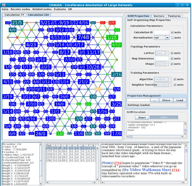
Figure 6.1 on the following page shows a screenshot of the Coalda GUI. The graph of
the SOM is displayed in the upper left of the GUI. When a user clicks a node, detailed information about this node is displayed in the lower part of the screen. This includes the weights of the node in the different input dimensions (left) as well as the feature vectors associated with the node (middle) and the text belonging to the feature vectors (right). The text corresponding to the feature vectors is shown in a simple text-based visualization. A markable is enclosed in square brackets []. The number right after the closing bracket is the ID of the feature vector the markable belongs to. There can be multiple IDs for one markable. If the feature vector is labeled as coreferent, the ID is green. If the feature vector is labeled as disreferent, the ID is red. The text visualization component will be provided by Andre Burkovski.
The color of the nodes is initially the U-matrix value. The color can be changed to represent the weight of the node in a selected feature. It can also be changed to show the percentage of coreferent feature vectors in this node, if there already are labeled feature vectors. Every node has a node-label which is initially the ID of the node. This node-label can contain the number of feature vectors associated with this node. It can also indicate how many of these feature vectors are labeled as co- or disreferent.
6 The Coalda Software
Figure6.1: Coalda GUI
With a double click on a node, all feature vectors associated with that node can be assigned a label. The label can have a confidence value. It is not possible to assign a label to a single feature vector.
If a user wants to see a part of the SOM in more detail, he can either zoom in on one node or select several nodes and recalculate a SOM for this selection. In both cases a new SOM is calculated for the feature vectors associated with the selected node(s) and the result of the calculation is visualized in a new tab.
6.3 Architectural Design
Figure6.2: Architecture of the prefuse Visualization Framework [HCL05]
The SOM can also be recalculated for all the feature vectors with a different configuration of the SOM or with a subset of the features used for the first calculation. These settings can be changed in the panel at the right hand side of the screen.
The calculation of the SOM will be performed by a Matlab SOM server. The communication with the Matlab SOM server will be implemented by Andre Burkovski.
6.3 Architectural Design
The visualization is based on the prefuse visualization framework1
for Java. The architecture of this framework as presented in [HCL05] is shown in figure6.2.
The data to be visualized is taken from some source and converted to prefuse abstract data items. The data items are converted to visual items by adding the information necessary for visualization. Action lists can influence the visual appearance of visual items, for example the size or the color. Actions can also change the layout.
Visual items are drawn on the display by a renderer. UI controls can be added to the display to make the visualization interactive. These UI controls can trigger changes in any part of the system.
The parts to implement and to adapt for the Coalda software are I/O Libraries, Action Lists and UI Controls. Other components are taken from default prefuse libraries, for example the renderer or the UI Control for dragging.
6 The Coalda Software
6.3.1 I/O Libraries
The modules that implement I/O libraries work on the data in the project database. The data to be loaded is of three types: data for calculations, feature vectors and labels. Consequently, a module for each type has been implemented. Data from calculations and feature vectors only needs to be loaded. Labels need to be loaded and written back into the database. The modules to be implemented are the following:
CalculationImport Takes the data out of the database and converts it to a prefuse abstract data item. The data to be imported is the result of a calculation. This includes the nodes of the SOM and for every node the U-matrix value, the weights in the different input space dimensions and the associated feature vectors. For edges only the U-matrix value needs to be imported.
Input: Data from calculation table in the project database.
Output: Prefuse abstract data items.
FeatureVectorImport Responsible for loading the feature vectors associated with a node and the text belonging to the feature vectors.
Input: Data from feature vector table in the project database.
Output: Screen display of feature vectors and text.
LabelImport Responsible for getting the label of one or several feature vectors.
Input: Data from link table in the project database.
Output: Label of feature vector(s).
LabelExport Writes the label a user assigned to the feature vectors associated with this node into the data base.
Input: User Input.
Output: Entry in link table in the project database.
Learner The SOM is calculated by Matlab2
using the SOM Toolbox for Matlab3
[VHAP00].
The implementation of the classes for the connection to Matlab as well as the classes for the configuration of Matlab was provided by Andre Burkovski in the packagesomserver.
All these classes are contained in the moduleLearner. Once a calculation is finished,
the actual loading is done by the moduleCalculationImport. Input: SOM Configuration.
Output: Calculation ID to be loaded.
Uses: CalculationImport
6.3.2 ActionLists
Action lists are used to determine the appearance of visual items on the display. Action lists can influence layout, color, node-label and size. It can be specified when an action list should be run. The action lists to be defined are the following:
2
http://www.mathworks.com/products/matlab
3
http://www.cis.hut.fi/projects/somtoolbox/
6.3 Architectural Design LayoutAction The basic layout is a two-dimensional grid based on the positions of the SOM
nodes in output space.
Runs after: CalculationImport
ColorAction The color of an edge is its U-matrix value. The color of a node is determined by the field the user has selected. Initially this field is set to be the U-matrix value. Selected nodes are highlighted in a color different from that of other nodes.
Runs after: CalculationImport,Selection,RecolorNodes
NodeLabelAction The node-label of a node is determined by the field the user has selected. Initially this field is set to be the ID of the node.
Runs after: CalculationImport,RelabelNodes
SizeAction Size of nodes is partially determined by the space the label requires. Other than that, size is determined by the number of feature vectors associated with a node.
Runs after: CalculationImport
6.3.3 UI Controls
Every UI module implements a single functionality. Several UI functionalities can be triggered by the same user action. User actions can trigger changes in any part of the system. The controls to be implemented are the following:
Selection When a user selects a node by clicking on it, the color of this node is changed to indicate that the node is selected. The nodes of the previous selection are not highlighted anymore.
Trigger: Click on any node.
Result: Current node is highlighted.
Uses: ColorAction
Focus When a user selects a node by clicking on it, additional information is displayed. This includes information about the node, about the associated feature vectors and the text associated with the feature vectors.
Trigger: Click on a node that has associated feature vectors.
Result: Information about current node is displayed.
Uses: FeatureVectorImport
Labeling When a user double clicks a node, he can assign a label to all feature vectors associated with this node. This label has an associated confidence value also assigned by the user.
Trigger: Double click on any node.
Result: All feature vectors associated with the current node are assigned the label chosen by the user with the confidence value chosen by the user.
Uses: LabelExport
SOMZoom This control contacts the Matlab SOM server, which calculates a new SOM for the feature vectors of the node the user has zoomed in on. Zoom does not work on edges or nodes with no feature vectors associated. The visualization of the new calculation
6 The Coalda Software
opens in a new tab.
Trigger: Zoom in on a node that has associated feature vectors.
Result: A new tab opens containing the visualization of a SOM calculated with the feature vectors associated with the current node.
Uses: Learner
Recalculate Contacts the Matlab SOM server, which calculates a new SOM with the current settings. Modified settings can affect the feature vectors, the features or the SOM configuration used for the calculation.
Trigger: Click buttonStart.
Result: A new tab opens containing a new SOM calculated with the current settings.
Uses: Learner
RecolorNodes Updates the color of all nodes according to the selected field.
Trigger: Select different field in menuRecolor.
Result: All nodes are colored according to their value in the selected field.
Uses: ColorAction
RelabelNodes Updates the node-label of all nodes according to the selected field.
Trigger: Select different field in menuRelabel.
Result: All nodes are labeled according to their value in the selected field.
Uses: NodeLabelAction
LoadCalculation Loads a specific (previously stored) calculation from the database.
Trigger: Select menu itemLoadfrom menuData.
Result: A new tab opens containing the calculation to be loaded.
Uses: CalculationImport
![Figure 6.2: Architecture of the prefuse Visualization Framework [HCL05]](https://thumb-us.123doks.com/thumbv2/123dok_us/10760914.2964237/39.892.93.733.180.388/figure-architecture-prefuse-visualization-framework-hcl.webp)