Exchange Rate Volatility and Trade Flows
1Ali Eren ALPER 2
ARTICLE INFO ABSTRACT
Article History:
Date Submitted: 20.04.2017 Date Accepted: 30.04.2017
After the collapse of Bretton-Woods system in 1973, many countries adopted the floating exchange rate regime. This situation led to fluctation and uncertainties in the exchange rates. There are number of studies that analyze the effect of Exchange rate volatility on trade flows but previous studies cannot obtain results about sectoral base due to the lack of disaggregated data sets. This study investigates the effects of exchange rate volatility on trade flows in Turkey. For this purpose using annual data covers the period 2002-2013. Exports to 15 European countries and imports from 15 European countries are analyzed by panel methodology. According to the test results, export sectors are negatively affected; import sectors are both positively and negatively affected from exchange rate volatility.
JEL Classification:
F10 F31 C23
Keywords:
Exchange Rate Volatility Trade Flows
Panel Data Analysis
1 This paper is derived from the Ph. D. thesis titled with “Exchange Rate Volatility and Trade Flows” at Institute
I. Introduction
Exchange rates are among the major determinants of foreign trade. They have the ability of influencing trade flows all around the globe. Foreign exchange rates have been highly volatile since the currencies of the major industrial countries were allowed to float in 1973. When fixed rates abandoned, many observers thought exchange rate fluctuations would eventually dampen as market participants gained experience in flexibly priced currency markets.
Exchange rate volatility is a cause for concern if it impairs the smooth functioning of the world economy. Volatility can be detrimental in several ways. It can reduce the volume of international trade by creating uncertainty about the profits to be made from international transactions. Fluctuations in exchange rates also might restrict the international flow of capital by reducing both direct investment in foreign operating facilities and financial portfolio investment. Finally, exchange rate volatility might lead to higher prices for internationally traded goods by causing traders to add a risk premium to cover unanticipated exchange rate fluctuations.
Volatility of exchange rates can also restrict the flow of international capital by reducing direct and portfolio investments. Speculative capital flows may also be induced by exchange rate volatility under the flexible regime that could in turn contribute to the instability in economic conditions. Greater exchange rate volatility increases uncertainty over the return of a given investment. Potential investors are attracted to invest in a foreign location as long as the expected returns are high enough to compensate for the currency risk.
There is growing and firm evidence that exchange rate volatility imposes significant effects on the volume of trade. This evidence is borne out of a variety of empirical tests that have been conducted over the years. Exchange rate variability affects international specialization in production which in turn leads to a reduction in the welfare of people as output declines and consequently income and consumption. Volatility in the exchange rate can lead to the reduction in the volume of international trade due to increases in the level of trade riskiness that creates uncertainty about profits. In addition, it causes prices of tradable to rise to the risk
mark-up (risk premium) imposed by sellers in order to protect profits. This tends to affect the competitiveness of exports. In response to fluctuations in the exchange rate, firms shift resources from the risky tradable sector to the less risky non-tradable sector in order to protect their profits. Further, a rise in exchange rate uncertainty increases transaction costs as agents attempt to hedge against exchange rate risk.
In view of these potential problems, this paper investigates the effects of exchange rate volatility on Turkish imports and exports during the 2002-2013 period by using the panel data estimation procedure.
2. Literature Review of Flexible Exchange Rates and International Trade
The volatility of flexible exchange rates can inflict damage on businesses and economies at large. Although the associated costs have not been quantified rigorously, many economists believe that exchange rate uncertainty reduces welfare-enhancing international trade and discourages investments.
Following the seminal work of Hooper and Kohlhagen (1978), a large amount of research has been published in an attempt to discover a robust relationship between exchange rate variability and international trade. Early empirical research suggested that there was no statistically significant variability effect. A now well-known quote from the International Monetary Fund (IMF) (1984) states:
“The large majority of empirical studies on the impact of exchange rate
variability on the volume of international trade are unable to establish a systematically significant link between measured exchange rate variability and the volume of international trade, whether on an aggregated or on a
bilateral basis”(IMF, 1984, p.36)
Since the appearance of IMF (1984) study of the effects of exchange rate volatility on trade, two survey papers of the literature on the topic have appeared: Cote (1994) and McKenzie (1999). These two surveys conclude that from a theoretical perspective there is no unambiguous response in the level of trade to an increase in exchange rate volatility, as differing results can
arise from plausible alternative assumptions and modelling strategies. The same ambiguity pervades much of the empirical literature, which may reflect the lack of clear cut theoretical results as well as the difficulty in arriving at an appropriate proxy for exchange rate risk.
Makin (1978), a finance perspective suggests that there are many possibilities for a multinational corporation to hedge foreign currency risks arising from exports and imports by holding a portfolio of assets and liabilities in different currencies.
Hooper and Kohlhagen (1978) utilized a model for traded goods and derived equations for export prices and quantities in terms of the costs of production reflecting both domestic and imported inputs, other domestic prices, domestic income and capacity utilization. Exchange rate risk was measured by the average absolute difference between the current period spot exchange rate and forward rate last period. They examined the impact of exchange rate volatility on aggregate and bilateral trade flow data for all G-7 countries except Italy. In terms of the effect of volatility on trade flows, they found essentially no evidence of any negative effect.
Baum, Çağlayan and Özkan (2004) investigate empirically the impact of exchange rate
volatility on real international trade flows utilizing a 13 country data set of monthly bilateral real exports for 1980-1998. They compute one month ahead exchange rate volatility from the intra-monthly variations in the exchange rate to better quantify this latent variable. They find the effect of exchange rate volatility on trade flows in nonlinear, depending on its interaction with the importing country’s volatility of economic activity, and that it varies considerably over the set of country pairs considered.
Tenreyro (2007) investigates broad sample of countries from 1970 to 1997 and argues that all potential sources of bias should be tackled simultaneously and that partial corrections can be highly misleading. The writer hence develops a Poisson pseudo maximum likelihood
(PPML) approach that addresses the various potential biases. The instrument that used in the
paper relies on the fact that many countries find it useful to peg their currency to that of a large and stable anchor country in order to reduce inflation. The estimates indicate that nominal exchange rate variability has no significant impact on trade flows.
Baak (2008) examines the impacts of the real exchange rates between the renminbi and the US dollar on the trade between the two countries. The impacts of the real bilateral exchange rate on the Chinese exports to the US and on the US exports to China were measured by estimating cointegrating vectors and error correction models. The impact of other variables, such as the exchange rate of a competing country, the real gross domestic product (GDP) of the importing country, the volatility of the exchange rate between the renminbi and the dollar, were also measured by including them as explanatory variables along with the exchange rate between the renminbi and the dollar in the export functions. The results show that volatility of exchange rates turned out to negatively influence the Chinese exports to the US, but not to have any
influences on the US exports to China. The coefficient values of the real GDP’s were estimated
to be positive and bigger than the coefficient values of the exchange rates, implying income elasticity is higher than price elasticity in the export functions.
Rahman and Serletis (2009) investigate the effects of exchange rate uncertainty on exports in the context of a multivariate framework. Their measure of exchange rate uncertainty is the conditional standard deviation of the forecast error of the change in the exchange rate. They estimate the model using aggregate monthly data for the US over the flexible exchange rate period since 1973:1 to 2007:1. They find that exchange rate uncertainty statistically and economically significantly affects exports. They also find that accounting for uncertainty about exchange rate movements tends to augment the negative dynamic response of exports to a positive exchange rate shock.
Baum and Çağlayan (2010) present an empirical investigation of the hypotheses that exchange rate uncertainty may have an impact on both the volume and variability of trade flows. Their investigation concentrates on bilateral trade flows between 13 countries including the US, UK, Canada, Germany, France, Italy Japan, Finland, Netherlands, Norway, Spain, Sweden and Switzerland for the period 1980-1998 on a monthly basis in each direction. The paper’s first result suggests that the impact of exchange rate volatility on trade flows is intermediate. Only a small number of models present significant relationship. Their second finding is the relationship between exchange rate volatility and trade flows. The writers argue that bilateral trade volatility is higher than GDP volatility.
Serenis and Serenis (2010) examine the potential effect of exchange rate volatility for a set of eleven EU member countries for sectoral trade exports of two products belonging to the chemical sector during the period of 1973-2005. The result of the writers’ estimation has proven that although for the most part exchange rate volatility does not have any major effects on the sectoral level of exports.
Zelekha and Efrat (2011) examine the effect of exchange rate uncertainty on Israeli exports of goods to the US. They use quarterly data for the period 1997:1-2010:1. Their results show that uncertainty has a negative and dominant effect on exports, in both the short run and the long run.
Verheyen (2012) tried to determine what effect such exchange rate volatility has on
exports from eleven euro zone countries to the US. The paper’s main result suggests that exchange rate volatility does exert a significant and negative effect on exports. Furthermore, the exports most often negatively affected seem to be those of SITC categories 6 and 7.
Poon and Hooy (2013) examine the impact of exchange rate volatility on trade in the Organization of the Islamic Conference (OIC) countries from 1995 to 2008 using panel estimations to distinguish differences between disaggregate trade and examine its threshold effects. Results overall corroborate the view that a mixed effect from volatility to exports. They document three main findings. First, results reveal that exports of OIC countries generally have significant and negative exposure to exchange rate volatility with small magnitude. Second, using lagged explanatory model, it is observed that there is significant marginal positive relationship between exchange rate volatility and import demand. Third, results also suggest evidence of a threshold effect.
And lastly Grier and Smallwood (2013) present an empirical analyze about exchange rate shocks and trade. They apply their methodology to a large data set, encompassing 27 countries. They use monthly data set runs from eight developed economies (Canada, Denmark, Japan, Norway, Sweden, Switzerland, the United Kingdom and the United States) and 19 less developed economies. In the less developed group, one is Eurasian (Turkey), two are on the Asian mainland (India and Pakistan), three are African continent (Morocco, Nigeria, South
Africa), six are Pacific Rim countries (Indonesia, Korea, Malaysia, the Philippines, Singapore and Thailand) and the remaining are Latin American (Argentina, Brazil, Chili, Ecuador, Mexico, Peru, Venezuela). In analyzing the effects of real exchange rate uncertainty, two sets of robust findings emerge. First, for the emerging economies in their sample, when significant effects are found, the link between uncertainty and export growth is always negative. Second real exchange rate uncertainty significantly impacts real exchange rate growth. If real appreciations are correlated with a reduction in trade, then their findings indicate that real exchange rate uncertainty negatively impacts export growth.
3. Data, Methodology and Empirical Results
Panel data methodology is used in the paper. For obtaining the coefficients of the variables, econometrical systemizing is as follows;
1. Cross sectional dependence (CSD) tests,
i. Pesaran’s CD Test
ii. Friedman’s Test
iii. Frees’ Test
2. Unit root test,
i. Cross Sectionally Augmented Dickey-Fuller Test 3. Cointegration test,
i. Westerlund (2008) Cointegration Test 4. If cointegrated, estimation of long run coefficients,
i. Common Correlated Effect Estimator
5. If not cointegrated, percentage transformation and the estimation of short run coefficients.
i. Feasible Generalized Least Squares Estimator
A growing body of panel data literature concludes that panel data models are likely to exhibit substantial cross sectional dependence in the errors, which may arise because of the presence of common shocks and unobserved components that ultimately become part of the error term, spatial dependence idiosyncratic pairwise dependence in the disturbances with no
particular pattern of common components or spatial dependence. The impact of cross sectional dependence in estimation naturally depends on a variety of factors, such as the magnitude of the correlations across cross sections and the nature of cross sectional dependence itself. Assuming that cross sectional dependence is caused by the presence of common factors, which are unobserved (and as a result, the effect of these components is felt through the disturbance term) but they are uncorrelated with the included regressors, the standard fixed effects (FE) and random effect (RE) estimators are consistent, although not efficient, and the estimated standard errors are biased. In this case different possibilities arise in estimation. On the other hand, if the unobserved components that create interdependencies across cross sections are correlated with the included regressors, these approaches will not work and the FE and RE estimators will be biased and inconsistent.
In all three tests, under the null hypothesis 𝑢𝑖𝑡 is assumed to be independent and identically distributed (i.i.d) over time periods and across cross sectional units. Under the alternative 𝑢𝑖𝑡 may be correlated across cross sections.
Thus hypotheses are,
𝐻0 = 𝜌𝑖𝑗 = 𝜌𝑗𝑖 = 𝑐𝑜𝑟 (𝑢𝑖𝑡, 𝑢𝑗𝑡) = 0 𝑓𝑜𝑟 𝑖 ≠ 𝑗 𝐻1 = 𝜌𝑖𝑗 = 𝜌𝑗𝑖 ≠ 0 𝑓𝑜𝑟 𝑖 ≠ 𝑗
The use of panel cointegration techniques to test for the presence of long-run relationships among integrated variables with both a time series dimension T and a cross sectional dimension N has received much attention recently. The literature concerned with the development of such tests has thus far taken two broad directions. The first consists of taking cointegration as the null hypothesis. The second approach is to take no cointegration as the null hypothesis (Westerlund, 2008).
But cointegration techniques require the data sets which have to be non-stationary. If one of the variables is stationary, these techniques do not work. Westerlund solved this drawback with his seminal paper.
Westerlund’s (2008) main objective is to test whether 𝑖𝑖𝑡 and 𝜋𝑖𝑡 are cointegrated or not by inferring whether 𝑒𝑖𝑡 is stationary or not. A natural approach to do this is to employ Bai and Ng (2004) approach. A test of the null hypothesis of no cointegration can then be implemented as a unit root test of the recumulated sum of the defactored and first differentiated residuals. The first advantage of this test has small size distortions and greater power than other popular panel cointegration tests. Second advantage is with the test is that they are robust against the presence of stationary regressors. Third advantage is that the test can be readily implemented using a predetermined cointegration vector without affecting the asymptotic null distributions (Westerlund, 2008).
In assessing the impact of exchange rate volatility or risk on trade flows, all studies have used the import and export demand models in which exchange rate volatility as a measure of exchange rate risk is added to these models.
In examining the effect of exchange rate changes on trade flows at a bilateral level, economists typically rely on a theoretical framework developed by Bahmani-Oskooee and Wang (2008). In its simplest form this model can be stated as follows:
𝑉𝑋 = 𝑉𝑋(𝑌∗, 𝑅𝐸𝑅, 𝑉𝑂𝐿) 𝑉𝑀 = 𝑉𝑀(𝑌, 𝑅𝐸𝑅, 𝑉𝑂𝐿)
where VX (VM) is the value of real exports (imports) which is computed by nominal export (import) divided by price index, 𝑌∗ is the real gross dometic product (GDP) of the 15 (France, Netherlands, Germany, Italy, United Kingdom, Denmark, Greece, Portugal, Spain, Belgium, Sweden, Austria, Poland, Czech Republic, Romania) European countries (which these countries have %93 share of Turkish exports to Europe and imports from Europe) RER is the real effective exchange rate, and VOL is the volatility of exchange rate which is computed using by GARCH (1, 0).
The variables used in the analysis are constructed as above. Export and import data (Standard International Trade Statistics Revision 3) are collected from Turkish Statistical
Institute for two digit frequency (TUIK), GDP and RER datas are collected from Eurostat. The analysis was conducted on a yearly basis and started from 2002 to 2013.
Thus following the literature (e.g. Bahmani-Oskooee and Wang, 2008; Baek, 2013; Nishimura and Hirayama, 2013) the study assume that Turkish export of commodity i to 15 European countries takes the following specification:
𝑙𝑛𝑋𝑖,𝑡 = 𝛽0+ 𝛽1𝑙𝑛𝑌𝐸𝑢,𝑡+ 𝛽2𝑙𝑛𝑅𝐸𝑅𝑡+ 𝛽3𝑙𝑛𝑉𝑂𝐿𝑡+ 𝜀𝑖,𝑡
where 𝑋𝑖,𝑡 is real export volume of commodity i to country t which is assumed to depend positively on European real income, 𝑌𝐸𝑈,𝑡. The real effective exchange rate is denoted by RER. Real depreciation of Turkish Lira against Euro reflects the appreciation of RER. Therefore, if real depreciation of the Turkish Lira is to stimulate Turkish export of commodity i. Finally, if an increase in the measure of exchange rate variability, VOL, is to hurt exports.
So in this export demand equation expected signs of the coefficients are as follows:
𝛽1 > 0, 𝛽2 > 0 𝛽3 < 0
To assess the impact of exchange rate volatility on Turkish imports from European countries, the study assume that Turkish import demand for commodity i from country t takes the following form:
𝑙𝑛𝑀𝑖,𝑡 = 𝛼0+ 𝛼1𝑙𝑛𝑌𝑇𝑅 + 𝛼2𝑙𝑛𝑅𝐸𝑅𝑡+ 𝛼3𝑙𝑛𝑉𝑂𝐿𝑡+𝜀𝑖,𝑡
where 𝑀𝑖,𝑡 is the import volume of commodity i by Turkey from European countries which is assumed to have a positive relation with Turkish real income. The real effective exchange rate is negatively related with import volume. Because, the appreciation of Turkish Lira depreciates the RER, so imported goods from European countries become cheaper, due to
this situation depreciation of RER is expected to boost Turkish imports. Finally, exchange rate variability is expected to deter imports.
Therefore, in this import demand equation expected signs of the coefficients are as follows:
𝛼1 > 0 𝛼2 < 0 𝛼3 < 0
At the beginning of the empirical analysis, the study first concentrate the cross sectional dependency (CSD) tests. CSD tests are so important because these test results determined that the use of first or second generation unit root and cointegration tests. If CSD tests detected a cross sectional dependency second generation unit root and cointegration techniques are used at the further stages, otherwise first generation techniques are used.
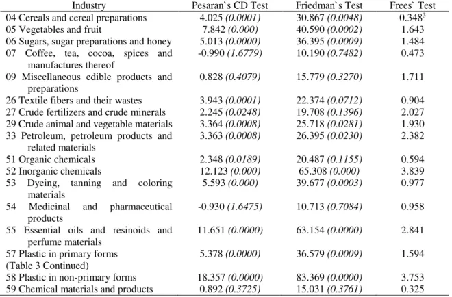
Table 1: Cross Sectioanlly Dependence Tests of Export Industries (Probability Values Are in the Parenthesis)
Industry Pesaran`s CD Test Friedman`s Test Frees` Test 04 Cereals and cereal preparations 4.025 (0.0001) 30.867 (0.0048) 0.3483 05 Vegetables and fruit 7.842 (0.000) 40.590 (0.0002) 1.643 06 Sugars, sugar preparations and honey 5.013 (0.0000) 36.395 (0.0009) 1.484 07 Coffee, tea, cocoa, spices and
manufactures thereof
-0.990 (1.6779) 10.190 (0.7482) 0.473 09 Miscellaneous edible products and
preparations
0.828 (0.4079) 15.779 (0.3270) 1.711 26 Textile fibers and their wastes 3.943 (0.0001) 22.374 (0.0712) 0.904 27 Crude fertilizers and crude minerals 2.245 (0.0248) 19.708 (0.1396) 2.027 29 Crude animal and vegetable materials 3.364 (0.0008) 25.718 (0.0281) 1.930 33 Petroleum, petroleum products and
related materials
3.363 (0.0008) 26.395 (0.0230) 2.382 51 Organic chemicals 2.348 (0.0189) 20.487 (0.1155) 0.594 52 Inorganic chemicals 12.123 (0.000) 65.308 (0.000) 3.839 53 Dyeing, tanning and coloring
materials
5.593 (0.000) 39.677 (0.0003) 0.977 54 Medicinal and pharmaceutical
products
-0.930 (1.6475) 10.713 (0.7084) 0.958 55 Essential oils and resinoids and
perfume materials
11.651 (0.0000) 63.154 (0.0000) 2.841 57 Plastic in primary forms 5.378 (0.0000) 36.579 (0.0009) 1.594 (Table 3 Continued)
58 Plastic in non-primary forms 18.357 (0.0000) 83.369 (0.0000) 3.753 59 Chemical materials and products 0.892 (0.3725) 15.031 (0.3761) 0.325
61 Leather, leather manufactures and dressed fur skins
0.456 (0.6485) 15.297 (0.3581) 0.786 62 Rubber manufactures 7.973 (0.0000) 48.015 (0.0000) 3.252 63 Cork and wood manufactures 0.773 (0.4398) 16.169 (0.3031) 0.728 64 Paper, paperboard and articles of
paper pulp
4.209 (0.0000) 28.723 (0.0114) 1.518 65 Textile yarn, fabrics, made-up articles
and related products
7.321 (0.0000) 41.605 (0.0001) 1.508 66 Non-metallic mineral manufactures 1.504 (0.1325) 22.149 (0.0756) 2.421 67 Iron and steel 4.220 (0.0000) 27.390 (0.0171) 0.939 68 Non-ferrous metals 13.736 (0.0000) 74.446 (0.0000) 2.736 69 Manufactures of metals 9.030 (0.0000) 47.646 (0.0000) 1.272 (Table 1 continued)
Industry Pesaran`s CD Test Friedman`s Test Frees` Test 71 Power generating machinery and
equipment
0.655 (0.5127) 14.344 (0.4244) 0.898 72 Machinery specialized for particular
industries
3.470 (0.0005) 25.082 (0.0338) 0.340 73 Metalworking machinery 5.955 (0.0000) 36.538 (0.0009) 1.171 74 General industrial machinery and
equipment
8.391 (0.0000) 51.297 (0.0000) 2.267 75 Office machines and automatic data
processing machines
-0.125 (1.1703) 10.631 (0.7148) 0.338 76 Telecommunications and sound
recording apparatus
13.522 (0.0000) 73.010 (0.0000) 2.811 77 Electrical machinery, apparatus and
appliances
4.729 (0.0000) 32.569 (0.0033) 0.851
78 Road vehicles 6.566 (0.0000) 42.015 (0.0001) 0.874
79 Other transport equipment 2.754 (0.0059) 23.092 (0.0588) 0.616 81 Prefabricated buildings, sanitary,
plumbing, heating and lighting
2.916 (0.0036) 23.779 (0.0487) 1.326 82 Furniture and parts thereof 2.394 (0.0167) 21.954 (0.0796) 2.401 83 Travel goods, handbags and similar
containers
6.162 (0.0000) 38.108 (0.0005) 1.963 84 Articles of apparel and clothing
accessories
-0.050 (1.0396) 9.277 (0.8129) 3.026
85 Footwear 2.585 (0.0097) 24.138 (0.0441) 0.771
87 Professional, scientific and controlling instruments
6.412 (0.0000) 37.728 (0.0006) 1.091 88 Photographic apparatus, equipment
and supplies and optical goods
2.550 (0.0108) 22.456 (0.0697) 0.476 89 Miscellaneous manufactured articles 4.618 (0.0000) 27.585 (0.0161) 1.212
In all 43 two digit industries, at least one test determines the cross section dependency. In particular, among 43 two stage industries, cross sectional dependency of 27 industries is
approved with all three tests. 12 of theme’s cross sectional dependency is approved with one
After CSD tests, we apply to all 43 industries, a second generation cointegration test. These results show us, if an industry is cointegrated, it means that we can estimate the long-run coefficients with that panel, otherwise we have to estimate short run coefficients.
Westerlund panel cointegration test results are pointed out below:
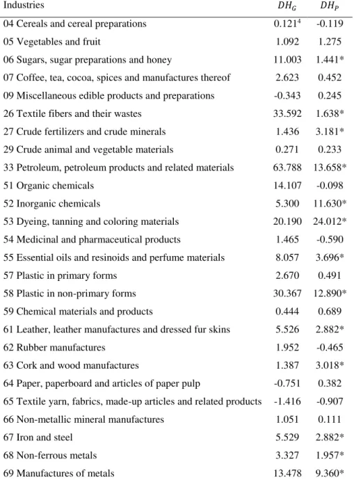
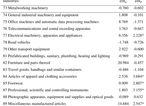
Table 2: Westerlund Panel Cointegration Test Results of Export Industries
Industries 𝐷𝐻𝐺 𝐷𝐻𝑃
04 Cereals and cereal preparations 0.1214 -0.119
05 Vegetables and fruit 1.092 1.275
06 Sugars, sugar preparations and honey 11.003 1.441* 07 Coffee, tea, cocoa, spices and manufactures thereof 2.623 0.452 09 Miscellaneous edible products and preparations -0.343 0.245 26 Textile fibers and their wastes 33.592 1.638* 27 Crude fertilizers and crude minerals 1.436 3.181* 29 Crude animal and vegetable materials 0.271 0.233 33 Petroleum, petroleum products and related materials 63.788 13.658*
51 Organic chemicals 14.107 -0.098
52 Inorganic chemicals 5.300 11.630*
53 Dyeing, tanning and coloring materials 20.190 24.012* 54 Medicinal and pharmaceutical products 1.465 -0.590 55 Essential oils and resinoids and perfume materials 8.057 3.696*
57 Plastic in primary forms 2.670 0.491
58 Plastic in non-primary forms 30.367 12.890* 59 Chemical materials and products 0.444 0.689 61 Leather, leather manufactures and dressed fur skins 5.526 2.882*
62 Rubber manufactures 1.952 -0.465
63 Cork and wood manufactures 1.387 3.018*
64 Paper, paperboard and articles of paper pulp -0.751 0.382 65 Textile yarn, fabrics, made-up articles and related products -1.416 -0.907 66 Non-metallic mineral manufactures 1.051 0.111
67 Iron and steel 5.529 2.882*
68 Non-ferrous metals 3.327 1.957*
69 Manufactures of metals 13.478 9.360*
71 Power generating machinery and equipment -0.764 -1.431 72 Machinery specialized for particular industries 1.632 2.974* (Table 2 Continued)
Industries 𝐷𝐻𝐺 𝐷𝐻𝑃
73 Metalworking machinery -0.760 -0.602
74 General industrial machinery and equipment 1.808 -0.101 75 Office machines and automatic data processing machines 8.769 -1.371 76 Telecommunications and sound recording apparatus 3.763 -0.667 77 Electrical machinery, apparatus and appliances 6.356 2.228*
78 Road vehicles -1.748 -0.726
79 Other transport equipment 2.922 -0.600
81 Prefabricated buildings, sanitary, plumbing, heating and lighting -0.969 -0.291
82 Furniture and parts thereof 20.984 -0.457
83 Travel goods, handbags and similar containers -0.486 -1.104 84 Articles of apparel and clothing accessories 2.538 3.684*
85 Footwear 0.909 2.807*
87 Professional, scientific and controlling instruments 1.803 3.155* 88 Photographic apparatus, equipment and supplies and optical goods -0.089 0.632 89 Miscellaneous manufactured articles 14.684 2.547*
Westerlund panel cointegration test results indicate that 06, 26, 27, 33, 52, 53, 55, 58, 61, 63, 67, 68, 69, 72, 77, 84, 85, 87, and 89 coded industries are cointegrated, the others are not cointegrated.
Finally, we first estimate short run coefficients with the industries which are not cointegrated. For short run coefficient, the study use Feasible Generalized Least Squares method.
Table 3: Short Run Coefficients of Export Industries (Probability Values Are in Parenthesis)
Industry GDP RER VOL ST. DEV.
04 Cereals and cereal preparations -22,28 (0.00) 23.30 (0.00) 3.021 (0.217) 8.65 (0.142)
05 Vegetables and fruit -0.459 (0.818) 1.045 (0.000) -0.150 (0.001) -0.361 (0.002)
07 Coffee, tea, cocoa, spices, and manufactured thereof
0.547 (0.376) 0.738 (0.003) -0.409 (0.000) -0.893 (0.001)
29 Crude animal and vegetable materials
1.840 (0.029) -0.449 (0.127) -1.141 (0.000) -2.628 (0.000)
51 Organic chemicals 44.269 (0.000) -2.862 (0.036) -6.211 (0.000) -9.758 (0.000)
54 Medicinal and pharmaceutical products
0.971 (0.561) 3.738 (0.000) -0.276 (0.535) -0.846 (0.445)
57 Plastics in primary forms 7.059 (0.000) 0.644 (0.452) -0.342 (0.343) -1.571 (0.064)
59 Chemical materials and products -0.733 (0.796) 7.589 (0.000) -0.640 (0.113) 0.285 (0.761)
62 Rubber manufactures 3.210 (0.000) -0.434 (0.088) -0.077 (0.475) -0.0657 (0.806)
(Table 3 continued)
Industry GDP RER VOL ST.DEV.
65 Textile yarn, fabrics, made-up articles and related products
1.501 (0.000) -0.083 (0.435) -0.091 (0.042) -0.224 (0.049)
66 Non-metallic mineral manufactures
2.683 (0.000) -0.379 (0.000) -0.142 (0.001) -0.310 (0.003)
71 Power generating machinery and equipment
11.804 (0.000) -0.239 (0.761) -1.310 (0.000) -1.454 (0.020)
73 Metalworking machinery 6.550 (0.000) -0.203 (0.533) 0.401 (0.003) 1.331 (0.000)
74 General industrial machinery and equipment
2.540 (0.000) 0.374 (0.041) -0.055 (0.470) 0.179 (0.325)
75 Office machines and automatic data processing machines
9.305 (0.000) 2.701 (0.116) -0.335 (0.648) 1.756 (0.288)
76 Telecommunications and sound recording apparatus
2.469 (0.001) -0.667 (0.191) -0.060 (0.787) -0.154 (0.774)
78 Road vehicles 6.515 (0.000) 0.717 (0.000) -0.339 (0.000) -0.352 (0.038)
79 Other transport equipment 3.70 (0.000) 6.32 (0.000) 0.080 (0.993) -3.254 (0.899)
81Prefabricated buildings, sanitary, plumbing, heating and lighting fixtures
4.141 (0.000) -0.590 (0.000) -0.240 (0.000) -0.468 (0.000)
82 Furniture and parts thereof 3.060 (0.000) 0.191 (0.462) 0.023 (0.833) 0.130 (0.716)
83 Travel goods, handbags, and similar containers
6.052 (0.000) -0.849 (0.048) -0.369 (0.040) -1.304 (0.003)
88 Photographic apparatus, equipment and supplies and optical goods
5.942 (0.044) -4.356 (0.000) -0.655 (0.017) -2.980 (0.005)
As can be seen, there are 24 Turkish two digit industries in which four coefficients are computed. For brevity, we only report the short run coefficient estimates for measure of exchange rate variability which are VOL and ST. DEV. Furthermore, while the effects are changed, some of them is negative, some of them is positive. The results of the short run coefficient estimates of the export model show that 14 coefficient of the VOL and ST. DEV. variables are found to be statistically significant for same industries which are 05 Vegetables and fruit, 07 Coffee, tea, cocoa, spices, and manufactured thereof, 09 Miscellaneous edible
products and preparations, 29 Crude animal and vegetable materials, 51 Organic chemicals, 64 Paper, paperboard, and articles of paper pulp and dressed fur skins, 65 Textile yarn, fabrics, made-up articles and related products, 66 Non-metallic mineral manufactures, 71 Power generating machinery and equipment, 73 Metalworking machinery, 78 Road vehicles, 81 Prefabricated buildings, sanitary, plumbing, heating and lighting fixtures, 83 Travel goods, handbags, and similar containers, and lastly 88 Photographic apparatus, equipment and supplies and optical goods. And all 14 industries VOL and ST. DEV coefficients are all negative.
The table shown below shows the estimated long run coefficients by using Common
Correlated Effects Estimator (CCE).
Table 4: Long Run Coefficients of Export Industries (Probability Values Are in Parenthesis)
Industry GDP RER VOL
06 Sugars, sugar preparations and honey 1.325 (0.860) -0.153 (0.914) -48.964 (0.493)
26 Textile fibers and their wastes -1.015 (0.657) -0.044 (0.966) 16.111 (0.839)
27 Crude fertilizers, crude minerals -0.651 (0.839) -0.002 (0.997) -9.080 (0.858)
33 Petroleum, petroleum products and related materials
-18.541 (0.036) -0.412 (0.763) 87.032 (0.575)
52 Inorganic chemicals -0.002 (0.999) 0.209 (0.769) 29.671 (0.330)
53 Dyeing, tanning and coloring materials -0.370 (0.947) 0.037 (0.937) 28.397 (0.847)
55 Essential oils and resinoids and perfume materials, toilet, polishing preparations
-1.292 (0.646) 0.051 (0.887) -4.376 (0.914)
58 Plastics in non-primary forms -1.319 (0.531) -0.003 (0.981) -0.923 (0.982)
61 Leather, leather manufactures and dressed fur skins
4.786 (0.578) 0.097 (0.909) 7.352 (0.955)
63 Cork and wood manufactures -4.281 (0.361) -0.052 (0.963) -40.196 (0.757)
67 Iron and steel 7.741 (0.104) -0.144 (0.826) 3.360 (0.317)
68 Non-ferrous metals 2.249 (0.337) 0.148 (0.633) -19.093 (0.734)
69 Manufactures of metals -2.470 (0.026) 0.005 (0.998) -5.576 (0.857)
72 Machinery specialized for particular industries
2.643 (0.274) -0.183 (0.735) -16.719 (0.696)
77 Electrical machinery, apparatus and appliances
1.311 (0.489) -0.034 (0.922) 32.976 (0.597)
84 Articles of apparel and clothing accessories 1.102 (0.607) 0.157 (0.706) 18.178 (0.650)
85 Footwear 1.729 (0.532) -0.100 (0.843) 27.362 (0.601)
87 Professional, scientific and controlling instruments and apparatus
-1.312 (0.714) 0.076 (0.870) -32.559 (0.539)
89 Miscellaneous manufactured articles 4.345 (0.101) 0.167 (0.615) -8.675 (0.877)
From the long run coefficient estimates, the signs VOL variable of the 06 Sugars, sugar preparations and honey, 27 Crude fertilizers, crude minerals, 55 Essential oils and resinoids and perfume materials, toilet, polishing preparations, 58 Plastics in non-primary forms, 63 Cork and wood manufactures, 68 Non-ferrous metals, 69 Manufactures of metals, 72 Machinery
specialized for particular industries, 87 Professional, scientific and controlling instruments and apparatus, and 89 Miscellaneous manufactured articles are negative but statistically insignificant.
Signs of the VOL variable coefficients of the, 26 Textile fibers and their wastes, 33 Petroleum, petroleum products and related materials, 52 Inorganic chemicals, 53 Dyeing, tanning and coloring materials, 61 Leather, leather manufactures and dressed fur skins, 67 Iron and steel, 84 Articles of apparel and clothing accessories, and 85 Footwear, are positive but again statistically insignificant.
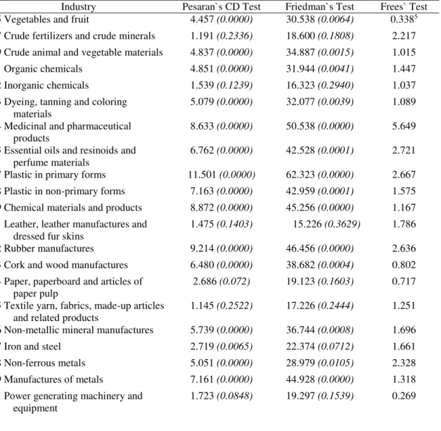
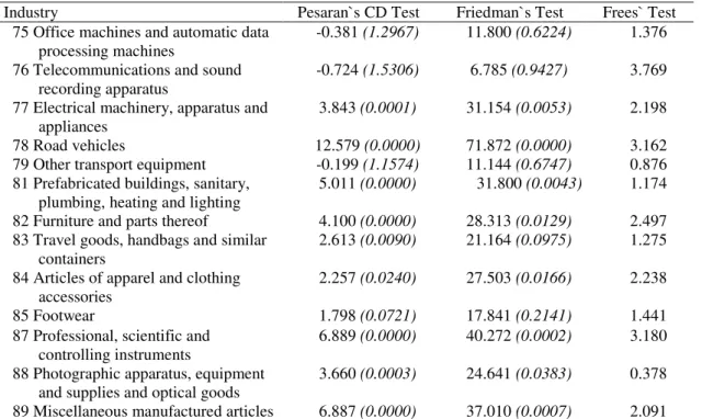
Table 5: Cross Sectional Dependence Tests of Import Industries (Probability Values Are in Parenthesis)
Industry Pesaran`s CD Test Friedman`s Test Frees` Test 05 Vegetables and fruit 4.457 (0.0000) 30.538 (0.0064) 0.3385 27 Crude fertilizers and crude minerals 1.191 (0.2336) 18.600 (0.1808) 2.217 29 Crude animal and vegetable materials 4.837 (0.0000) 34.887 (0.0015) 1.015 51 Organic chemicals 4.851 (0.0000) 31.944 (0.0041) 1.447 52 Inorganic chemicals 1.539 (0.1239) 16.323 (0.2940) 1.037 53 Dyeing, tanning and coloring
materials
5.079 (0.0000) 32.077 (0.0039) 1.089 54 Medicinal and pharmaceutical
products
8.633 (0.0000) 50.538 (0.0000) 5.649 55 Essential oils and resinoids and
perfume materials
6.762 (0.0000) 42.528 (0.0001) 2.721 57 Plastic in primary forms 11.501 (0.0000) 62.323 (0.0000) 2.667 58 Plastic in non-primary forms 7.163 (0.0000) 42.959 (0.0001) 1.575 59 Chemical materials and products 8.872 (0.0000) 45.256 (0.0000) 1.167 61 Leather, leather manufactures and
dressed fur skins
1.475 (0.1403) 15.226 (0.3629) 1.786 62 Rubber manufactures 9.214 (0.0000) 46.456 (0.0000) 2.636 63 Cork and wood manufactures 6.480 (0.0000) 38.682 (0.0004) 0.802 64 Paper, paperboard and articles of
paper pulp
2.686 (0.072) 19.123 (0.1603) 0.717 65 Textile yarn, fabrics, made-up articles
and related products
1.145 (0.2522) 17.226 (0.2444) 1.251 66 Non-metallic mineral manufactures 5.739 (0.0000) 36.744 (0.0008) 1.696 67 Iron and steel 2.719 (0.0065) 22.374 (0.0712) 1.661 68 Non-ferrous metals 5.051 (0.0000) 28.979 (0.0105) 2.328 69 Manufactures of metals 7.161 (0.0000) 44.928 (0.0000) 1.318 71 Power generating machinery and
equipment
1.723 (0.0848) 19.297 (0.1539) 0.269
72 Machinery specialized 11.592 (0.0000) 55.985 (0.0000) 2.485 73 Metalworking machinery
74 General industrial machinery and equipment 5.168 (0.0000) 12.962 (0.0000) 29.810 (0.0081) 68.928 (0.0000) 0.317 1.979 (Table 5 Continued)
Industry Pesaran`s CD Test Friedman`s Test Frees` Test 75 Office machines and automatic data
processing machines
-0.381 (1.2967) 11.800 (0.6224) 1.376 76 Telecommunications and sound
recording apparatus
-0.724 (1.5306) 6.785 (0.9427) 3.769 77 Electrical machinery, apparatus and
appliances
3.843 (0.0001) 31.154 (0.0053) 2.198 78 Road vehicles 12.579 (0.0000) 71.872 (0.0000) 3.162 79 Other transport equipment -0.199 (1.1574) 11.144 (0.6747) 0.876 81 Prefabricated buildings, sanitary,
plumbing, heating and lighting
5.011 (0.0000) 31.800 (0.0043) 1.174 82 Furniture and parts thereof 4.100 (0.0000) 28.313 (0.0129) 2.497 83 Travel goods, handbags and similar
containers
2.613 (0.0090) 21.164 (0.0975) 1.275 84 Articles of apparel and clothing
accessories
2.257 (0.0240) 27.503 (0.0166) 2.238
85 Footwear 1.798 (0.0721) 17.841 (0.2141) 1.441
87 Professional, scientific and controlling instruments
6.889 (0.0000) 40.272 (0.0002) 3.180 88 Photographic apparatus, equipment
and supplies and optical goods
3.660 (0.0003) 24.641 (0.0383) 0.378 89 Miscellaneous manufactured articles 6.887 (0.0000) 37.010 (0.0007) 2.091
In all 37 two digit industries, at least one test determines the cross section dependency. In particular, among 37 two stage industries, cross sectional dependency of 25 industries is
approved with all three tests. 10 of theme’s cross sectional dependency is approved with one
test and lastly 2 of the industries is approved is by two tests.
After CSD tests, we apply to all 37 industries a second generation cointegration test. These results show us, if an industry is cointegrated, it means that we can estimate the long-run coefficients with that panel, otherwise we have to estimate short run coefficients.
Westerlund panel cointegration test results are pointed out below:
Table 6: Westerlund Panel Cointegration Test Results of Import Industries
Industries 𝐷𝐻𝐺 𝐷𝐻𝑃
05 Vegetables and fruit 26.265 -0.415
29 Crude animal and vegetable materials -1.377 -1.278
51 Organic chemicals 15.296 4.619*6
52 Inorganic chemicals 2.027 -0.295
53 Dyeing, tanning and coloring materials -1.963 -0.266 54 Medicinal and pharmaceutical products 8.921 11.874* 55 Essential oils and resinoids and perfume materials 7.620 1.222
57 Plastic in primary forms -0.296 -1.798
58 Plastic in non-primary forms 11.373 6.726*
59 Chemical materials and products 0.611 -0.617
61 Leather, leather manufactures and dressed fur skins 0.608 4.388*
62 Rubber manufactures 73.536 1.010
63 Cork and wood manufactures 3.818 0.105
64 Paper, paperboard and articles of paper pulp 0.420 -1.600 65 Textile yarn, fabrics, made-up articles and related products -0.425 -1.989 66 Non-metallic mineral manufactures 135.133 7.195*
67 Iron and steel 27.673 1.737*
68 Non-ferrous metals 17.988 -1.507
69 Manufactures of metals 3.008 1.945*
71 Power generating machinery and equipment 1.912 0.779 72 Machinery specialized for particular industries 11.510 0.739
73 Metalworking machinery 3.979 7.301*
74 General industrial machinery and equipment 44.992 9.015* 75 Office machines and automatic data processing machines 5.897 -0.069 76 Telecommunications and sound recording apparatus -1.588 -1.047 77 Electrical machinery, apparatus and appliances -1.891 -1.044
78 Road vehicles 0.552 -0.682
79 Other transport equipment 2.906 -0.253
81 Prefabricated buildings, sanitary, plumbing, heating and lighting 1.041 2.282*
82 Furniture and parts thereof 0.861 0.308
83 Travel goods, handbags and similar containers 14.452 0.782 84 Articles of apparel and clothing accessories 10.055 12.359*
85 Footwear 1.436 1.920*
87 Professional, scientific and controlling instruments -2.363 -1.756 88 Photographic apparatus, equipment and supplies and optical goods 2.776 3.059* 89 Miscellaneous manufactured articles 44.386 4.176*
Westerlund panel cointegration test results indicate that 51, 54, 58, 61, 66, 67, 69, 73, 74, 81, 84, 85, 88, and 89 coded industries are cointegrated, the others are not cointegrated.
Finally, we first estimate short run coefficients with the industries which are not cointegrated. For short run coefficient, the study is used Feasible Generalized Least Squares method.
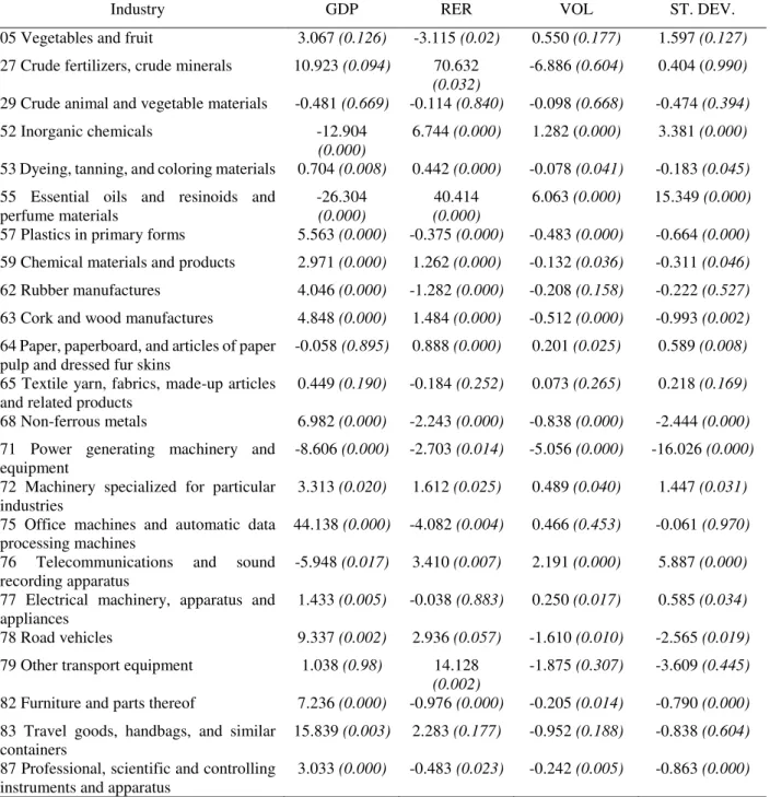
Table 7: Short Run Coefficients of Import Industries (Probability Values Are in Parenthesis)
Industry GDP RER VOL ST. DEV.
05 Vegetables and fruit 3.067 (0.126) -3.115 (0.02) 0.550 (0.177) 1.597 (0.127)
27 Crude fertilizers, crude minerals 10.923 (0.094) 70.632
(0.032)
-6.886 (0.604) 0.404 (0.990)
29 Crude animal and vegetable materials -0.481 (0.669) -0.114 (0.840) -0.098 (0.668) -0.474 (0.394)
52 Inorganic chemicals -12.904
(0.000)
6.744 (0.000) 1.282 (0.000) 3.381 (0.000)
53 Dyeing, tanning, and coloring materials 0.704 (0.008) 0.442 (0.000) -0.078 (0.041) -0.183 (0.045)
55 Essential oils and resinoids and perfume materials -26.304 (0.000) 40.414 (0.000) 6.063 (0.000) 15.349 (0.000)
57 Plastics in primary forms 5.563 (0.000) -0.375 (0.000) -0.483 (0.000) -0.664 (0.000)
59 Chemical materials and products 2.971 (0.000) 1.262 (0.000) -0.132 (0.036) -0.311 (0.046)
62 Rubber manufactures 4.046 (0.000) -1.282 (0.000) -0.208 (0.158) -0.222 (0.527)
63 Cork and wood manufactures 4.848 (0.000) 1.484 (0.000) -0.512 (0.000) -0.993 (0.002)
64 Paper, paperboard, and articles of paper pulp and dressed fur skins
-0.058 (0.895) 0.888 (0.000) 0.201 (0.025) 0.589 (0.008)
65 Textile yarn, fabrics, made-up articles and related products
0.449 (0.190) -0.184 (0.252) 0.073 (0.265) 0.218 (0.169)
68 Non-ferrous metals 6.982 (0.000) -2.243 (0.000) -0.838 (0.000) -2.444 (0.000)
71 Power generating machinery and equipment
-8.606 (0.000) -2.703 (0.014) -5.056 (0.000) -16.026 (0.000)
72 Machinery specialized for particular industries
3.313 (0.020) 1.612 (0.025) 0.489 (0.040) 1.447 (0.031)
75 Office machines and automatic data processing machines
44.138 (0.000) -4.082 (0.004) 0.466 (0.453) -0.061 (0.970)
76 Telecommunications and sound recording apparatus
-5.948 (0.017) 3.410 (0.007) 2.191 (0.000) 5.887 (0.000)
77 Electrical machinery, apparatus and appliances
1.433 (0.005) -0.038 (0.883) 0.250 (0.017) 0.585 (0.034)
78 Road vehicles 9.337 (0.002) 2.936 (0.057) -1.610 (0.010) -2.565 (0.019)
79 Other transport equipment 1.038 (0.98) 14.128
(0.002)
-1.875 (0.307) -3.609 (0.445)
82 Furniture and parts thereof 7.236 (0.000) -0.976 (0.000) -0.205 (0.014) -0.790 (0.000)
83 Travel goods, handbags, and similar containers
15.839 (0.003) 2.283 (0.177) -0.952 (0.188) -0.838 (0.604)
87 Professional, scientific and controlling instruments and apparatus
As can be seen, there are 23 Turkish two digit import industries in which four coefficients are computed. For brevity, we only report the short run coefficient estimates for measure of exchange rate variability which are VOL and ST. DEV. Furthermore, while the effects are changed, some of them is negative, some of them is positive. The results of the short run coefficient estimates of the import model show that 15 coefficient of the VOL and ST. DEV. variables are found to be statistically significant for same industries which are 52 Inorganic chemicals, 53 Dyeing, tanning, and coloring materials, 55 Essential oils and resinoids and perfume materials, 57 Plastics in primary forms, 59 Chemical materials and products, 63 Cork and wood manufactures, 64 Paper, paperboard, and articles of paper pulp and dressed fur skins, 68 Non-ferrous metals, 71 Power generating machinery and equipment, 72 Machinery specialized for particular industries, 76 Telecommunications and sound recording apparatus, 77 Electrical machinery, apparatus and appliances, 78 Road vehicles, 82 Furniture and parts thereof, 87 Professional, scientific and controlling instruments and apparatus.
The table shown below shows the estimated long run coefficients by using Common
Correlated Effects Estimator (CCE).
Table 8: Long Run Coefficients of Import Industries (Probability Values Are in Parenthesis)
Industry GDP RER VOL
51 Organic Chemicals 0.00135 (0.995) -0.0028 (0.786) -0.00015 (0.453)
54 Medicinal and pharmaceutical products
0.00597 (0.258) 0.0277 (0.367) -0.00013 (1.000)
58 Plastics in non-primary forms 0.00436 (1.000) -0.000571 (0.543) 0.00016 (1.000)
61 Leather, leather manufactures and dressed fur skins
0.000954 (0.127) 0.00861 (0.389) -0.0003 (1.000)
66 Non-metallic mineral manufactures -0.000782 (1.000) 0.000902 (1.000) 0.000053 (1.000)
67 Iron and steel 0.0000146 (1.000) 0.000234 (1.000) -0.00006 (0.275)
69 Manufactures of metals 0.00138 (1.000) 0.000694 (1.000) 0.00012 (1.000)
73 Metalworking machinery -0.000824 (0.147) 0.0000165 (1.000) 0.00013 (1.000)
74 General industrial machinery and equipment and machine parts
0.00192 (1.000) 0.00131 (1.000) 0.00020 (1.000)
81 Prefabricated buildings; sanitary, plumbing, heating and lighting fixtures
-0.000217 (0.496) 0.00346 (1.000) -0.00177 (1.000)
84 Articles of apparel and clothing accessories
85 Footwear -0.00465 (1.000) 0.00189 (1.000) 0.00039 (1.000)
88 Photographic apparatus, equipment and supplies and optical goods
0.00299 (0.635) -0.00162 (0.763) -0.00016 (1.000)
89 Miscellaneous manufactured articles -0.00337 (1.000) 0.00523 (0.489) 0.00031 (0.564)
From the long run coefficient estimates, the signs VOL variable of the, 51 Organic Chemicals, 54 Medicinal and pharmaceutical products, 61 Leather, leather manufactures and dressed fur skins, 67 Iron and steel, 81 Prefabricated buildings; sanitary, plumbing, heating and lighting fixtures, 88 Photographic apparatus, equipment and supplies and optical goods, are negative but statistically insignificant.
Signs of the VOL variable coefficients of the, 58 Plastics in non-primary forms, 66 Non-metallic mineral manufactures, 69 Manufactures of metals, 73 Metalworking machinery, 74 General industrial machinery and equipment and machine parts, 84 Articles of apparel and clothing accessories, 85 Footwear, 89 Miscellaneous manufactured articles, are positive but again statistically insignificant.
Conclusion
For countries that are open to foreign trade, the choice of optimal policy tool is the most important question when determining their foreign trade policies. Exchange rate is one of these policy tools. As being one of the main determinants of foreign trade, exchange rates can be used in influencing trade flows between countries. Change in exchange rates have the potential for correcting or damaging trade imbalances or balances.
Due to this fact the responsiveness of the trade balance to exchange rate changes is important because exchange rates do not only determine foreign trade but also influence national income in open economies. Understanding the dynamic relationship between exchange rate volatility and trade is a fundamental issue in open economy macroeconomics.
The main purpose of this paper was to investigate whether exchange rate volatility has any empirical influence on Turkish trade with European Union countries. By and large, studies have used such models only by employing aggregate trade data and have provided mixed results. Sector-level empirical studies are far scarcer then the aggregate ones. Such an aggregate
emphasis is defendable only under an assumption that impacts are homogenous across economic sectors.
Our main empirical findings can be summarized as follows;
In both export and import sectors, CSD tests Show us that all sectors are cross sectionally depended with each other. This means, unit root and cointegration tests which are used after this stage must be second generation.
After the CSD tests a second generation unit root test which is called CADF was used for determining the variables stationarity. The stationary test shows us that the GDP, RER and volatility variables are not stationary, but export and import variables change sector to sector.
Due to this station, to avoid spurious regression, for defining the cointegrated sectors Westerlund (2008) cointegration test was used. Unlike the other cointegration tests, this test do not need non-stationary for variables in the model. At least one non-stationary variable is sufficient for the analysis. Cointegration test results show that in the export model just 06, 26, 27, 33, 52, 53, 55, 58, 61, 63, 67, 68, 69, 72, 77, 84, 85, 87 and 89 coded and in the import model 51, 54, 58, 61, 66, 67, 69, 73, 74, 81, 84, 85, 88 and 89 coded industries are cointegrated.
After the identifying the cointegrated sectors, long run coefficients of these sectors by using CCE estimator. But as mentioned earlier in the long run all coefficients are statistically insignificant. Therefore, in the long run exchange rate volatility
does not affect Turkey’s trade with European Union countries.
The sectors, which are not cointegrated, has short run effects. These short run effects are computed by using FGLS estimator. 14 sectors through 24 Turkish two digit export industries, coefficients are found statistically significant for both GARCH (1, 0) and standard deviation volatility measures. These are 05 Vegetables and fruit, 07 Coffee, tea, cocoa, spices, and manufactured thereof, 09 Miscellaneous edible products and preparations, 29 Crude animal and vegetable materials, 51 Organic chemicals, 64 Paper, paperboard, and articles of paper pulp and dressed fur skins, 65 Textile yarn, fabrics, made-up articles and related products, 66
Non-Metalworking machinery, 78 Road vehicles, 81 Prefabricated buildings, sanitary, plumbing, heating and lighting fixtures, 83 Travel goods, handbags, and similar containers, and lastly 88 Photographic apparatus, equipment and supplies and optical goods. And all 14 industries volatility and standard deviation coefficients are all negative.
For the import sector 15 sectors through 24 Turkish two digit import industries, coefficients are found statistically significant for both volatility measures. These are 52 Inorganic chemicals, 53 Dyeing, tanning, and colouring materials, 55 Essential oils and resinoids and perfume materials, 57 Plastics in primary forms, 59 Chemical materials and products, 63 Cork and wood manufactures, 64 Paper, paperboard, and articles of paper pulp and dressed fur skins, 68 Non-ferrous metals, 71 Power generating machinery and equipment, 72 Machinery specialized for particular industries, 76 Telecommunications and sound recording apparatus, 77 Electrical machinery, apparatus and appliances, 78 Road vehicles, 82 Furniture and parts thereof, 87 Professional, scientific and controlling instruments and apparatus.
Unlike the export sector, import sector volatility coefficients are changed. 52, 55, 64, 72, 76, 77 code industries both volatility and standard deviation coefficients are positive; 53, 57, 59, 63, 68, 71, 78, 82, 87 coded import sectors volatility and standard deviation coefficients are negative.
REFERENCES
Baak, S. (2008). The bilateral real exchange rates and trade between China and the US. China
Economic Review, 19, 117-127.
Baek, J. (2013). Does the exchange rate matter to bilateral trade between Korea and Japan? Evidence from commodity trade data. Economic Modelling, 30, 856-862.
Bahmani-Oskooee, M. & Wang, Y. (2008). Impact of exchange rate uncertainty on commodity trade between the US and Australia. Australian Economic Papers, 47(3), 235-258. Bai, J. & Ng, S. (2004). A panic attack on unit roots and cointegration. Econometrica. 72. (4).
1127-1177.
Baum, C. F., Caglayan, M. & Ozkan, N. (2004). Nonlinear effects of exchange rate volatility on the volume of bilateral exports. Journal of Applied Econometrics, 19(1), 1-23. Baum, C. F. & Caglayan, M. (2010). On the sensitivity of the volume and volatility of bilateral
trade flows to exchange rate uncertainty. Journal of International Money and Finance, 29, 79-93.
Cote, A. (1994). Exchange Rate Volatility and Trade. Bank of Canada, Working Paper 94-5.
Frees, E. W. (1995). Assessing cross-sectional correlation in panel data.Journal of
econometrics, 69(2), 393-414.
Friedman, M. (1937). The use of ranks to avoid the assumption of normality implicit in the analysis of variance. Journal of the American Statistical Association, 32(200), 675-701.
Grier, K. B. & Smallwood, A. D. (2013). Exchange rate shocks and trade: A multivariate GARCH-M approach. Journal of International Money and Finance, 37, 282-305. Hooper, P., & Kohlhagen, S. W. (1978). The effect of exchange rate uncertainty on the prices
and volume of international trade. Journal of International Economics, 8(4), 483-511. International Monetary Fund (1984). Effects of exchange rate volatility on international trade
and other economic variables. IMF Occasional Paper No. 28.
Makin, J. H. (1978). Portfolio theory and the problem of foreign exchange risk. The Journal of
Finance, 33(2), 517-534.
McKenzie, M. D. (1999). The impact of exchange rate volatility on international trade flows. Journal of Economic Surveys, 13, No.1.
Nishimura, Y., & Hirayama, K. (2013). Does exchange rate volatility deter Japan-China trade? Evidence from pre- and post-exchange rate reform China. Japan and The World
Economy, 25-26, 90-101.
Pesaran, M. H. (2004). General diagnostic tests for cross section dependence in panels. CESifo Working Paper, No. 1229.
Poon, W. C. & Hooy, C. W. (2013). Exchange rate volatility, exchange rate regime, and trade in OIC countries. Journal of Asia-Pacific Business, 14(3), 182-201.
Rahman, S. & Serletis, A. (2009). The Effects of Exchange rate uncertainty on exports. Journal
of Macroeconomics, 31, 500-507.
Serenis, D. & Serenis, P. (2010). Exchange rate volatility, the EU and sectoral exports: New empirical evidence from the chemical sector. Research in World Economy, 1(1). Tenreyro, S. (2007). On the trade impact of nominal exchange rate volatility. Journal of
Development Economics, 82, 485-508.
Verheyen, F. (2012). Bilateral exports from euro zone countries to the US – Does exchange rate
variability play a role? International Review of Economics and Finance, 24, 97-108. Westerlund, J. (2008). Panel cointegration tests of the Fisher effect. Journal of Applied
Econometrics, 23, 193-233.
Zelekha, Y. & Bar-Efrat, O. (2011). The link between exchange rate uncertainty and Israeli exports to the US: 2SLS and cointegration approaches. Research in Economics, 65, 100-109.