Software performance modelling using PEPA nets

(1)

Software performance modelling using PEPA nets

Stephen Gilmore , Jane Hillston , Le¨ıla Kloul

and Marina Ribaudo

Laboratory for Foundations of Computer Science, The University of Edinburgh, Scotland

DISI — Dipartimento di Informatica e Scienze dell’Informazione, 16146 Genova, Italy

stg,jeh,[email protected] and [email protected]

ABSTRACT

Modelling and analysing distributed and mobile software sys-tems is a challenging task. PEPA nets—coloured stochas-tic Petri nets—are a recently introduced modelling formalism which clearly capture important features such as location, syn-chronisation and message passing. In this paper we describe PEPA nets and the newly-developed platform support for soft-ware performance modelling using them. Crucial to this sup-port is the compilation from PEPA nets into Hillston’s PEPA stochastic process algebra in order to access the software tools which support the PEPA algebra. In addition to derivation of steady state performance measures, this suite of tools allows properties of the system to be verified using model-checking. We show the application of PEPA nets in the modelling and analysis of a secure Web service.

Categories and Subject Descriptors

D.2.1 [ Software Engineering ]: Requirements / Specificat-ions — Methodologies ; D.3.2 [ Programming Languages ]: Language Classifications ; D.2.8 [ Software Engineering ]: Metrics—performance measures

General Terms

PEPA nets; performance analysis; mobile objects

1. INTRODUCTION

The correct representation of many modern software systems needs us to distinguish several distinct contexts of computa-tion. These contexts may depend on physical location, oper-ating conditions, or both. For example, in a distributed sys-tem interaction which takes place locally may be richer than that available through a remote interface; mobile objects may migrate within a system, significantly altering communication

On leave from PRISM, Universit´e de Versailles, 45, Av. des Etats-Unis 78000 Versailles, France.

Permission to make digital or hard copies of all or part of this work for personal or classroom use is granted without fee provided that copies are not made or distributed for profit or commercial advantage and that copies bear this notice and the full citation on the first page. To copy otherwise, to republish, to post on servers or to redistribute to lists, requires prior specific permission and/or a fee.

costs; and in fault-tolerant systems the current fault scenario can significantly affect performance.

Design decisions such as the placement of software compo-nents on hosts, the separation of client functions from server functions, and movement of code and data from host to host are typically motivated by the need to improve system reliabil-ity and performance. Unfortunately, many effective state-of-the-art performance analysis tools do not provide support, for example, for differentiating between simple local communica-tion and the movement or migracommunica-tion of processes which can change the allowable pattern of communication. One formal-ism which does separate these two mechanformal-isms is the PEPA

nets modelling language [1].

PEPA nets extend the PEPA stochastic process algebra [2] by allowing PEPA process algebra components to be used as the tokens of a coloured stochastic Petri net. A PEPA component has local state which can be modified by performing timed actions, either individually or in cooperation with another com-ponent. These activities define an interface analogous to the interface made up of the methods which can be invoked on an object. Constraints on the nature of the timing informa-tion (exponentially distributed random delays) mean that every PEPA model will define a Continuous-Time Markov Chain (CTMC). The addition of the Petri net infrastructure allows the modeller to represent explicitly locations or contexts (the statically-defined places of the net) and movement between them (the dynamically-determined firings of the net). Soft-ware components of the system, represented by PEPA compo-nents, make up the tokens of the net and move between the places of the net according to a formally defined firing rule. Furthermore, the semantics of the formalism imposes a restric-tion on communicarestric-tion based on the structure of the net. Com-munication is strictly confined within places—only compo-nents presently within the same context may interact. Thus interaction between tokens at different places is not allowed; for tokens to interact they must first meet at one of the places of the net. Moreover as a token moves around the net, its pos-sible activities may be altered to reflect its current location. Restricting communication according to these rules provides, for example, a credible formalism for representing mobile code systems where the tokens of a PEPA net model stateful mobile objects under a system of dynamic binding of names.

(2)

As explained above, the places of the PEPA net provide the locations, or contexts of the system. These are themselves modelled by PEPA components, termed static components, which, unlike tokens, are unable to move from the place. These immobile parts of the system may represent hardware (such as servers) or software (such as databases). Static components may communicate with tokens while they are present or they can communicate with other static components in the same place. Communication between static components at different places is not allowed.

In this paper we present PEPA nets, which have recently been extended to include more general net structures, and demon-strate their modelling and analysis capabilities on a small exam-ple of a mobile agent system and a more substantial case study based on a secure Web service.

There is an extensive suite of tools already supporting the PEPA language. In order to be able to exploit these tools, rather than develop new ones, we have developed an algorithm which compiles a PEPA net model to an equivalent model in PEPA. The difficulty here is transforming a PEPA net model into a model in a language which has no explicit notion of either location or mobility between locations. Despite the complex-ity of the transformation, we believe it is worthwhile since it provides access to established, trusted tools. Furthermore it is implemented in a software tool and therefore transparent to the user.

Structure of this paper: In the next section we present

exam-ples and the definition of the PEPA nets modelling language. This definition extends previous versions, by allowing a more general net structure to be used. We also explain the firing rule, which has been appropriately extended to take account of this more general structure. In Sect. 3 we describe the method of translating PEPA nets to PEPA and present results about the translation. In Sect. 4 we present an example of the algorithm. In Sect. 5 we describe the implementation of our translation method as an extension to the PEPA Workbench for PEPA nets which connects to the tools of the PEPA platform. The objec-tive of the algorithm is to allow PEPA net users to be able to exploit the existing tool support for PEPA. In Sect. 6 we give a brief overview of that tool support. In Sect. 7 we describe our Web Services case study. Conclusions are presented in Sect. 8.

2. PEPA NETS

In this section we provide a brief overview of PEPA nets and the PEPA stochastic process algebra. A fuller description, together with supporting theory and proofs is available in [1] and [2]. The purpose of this summary is to provide enough information about the modelling language to make the present paper self-contained.

The tokens of a PEPA net are terms of the PEPA stochastic pro-cess algebra which define the behaviour of components via the activities they undertake and the interactions between them. One example of a PEPA component would be a File object which can be opened for reading or writing, have data read (or written) and closed. Such an object would understand the methods openRead(), openWrite(), read(), write() and close().

A PEPA model shows the order in which such methods can be invoked. File def openReadro InStream openWritero OutStream InStream def readrr InStream closerc File OutStream def writerw OutStream closerc File

Every activity in the model incurs an execution cost which is quantified by an estimate of the (exponentially-distributed) rate at which it can occur (ro, rr, rw, rc).

Such a description documents a high-level protocol for using

File objects, from which it is possible to derive properties such

as “it is not possible to write to a closed file” and “read and write operations cannot be interleaved: the file must be closed and re-opened first”.

A PEPA net is made up of PEPA contexts, one at each place in the net. A context consists of a number of static components (possibly zero) and a number of cells (at least one). Like a memory location in an imperative program, a cell is a storage area to be filled by a datum of a particular type. In particular in a PEPA net, a cell is a storage area dedicated to storing a PEPA component, such as the File object described above. The components which fill cells can circulate as the tokens of the net. In contrast, the static components cannot move. A typical place might be the following:

File

L FileReader

where the synchronisation set L in this case is

File, the

complete action type set of the component, (openRead, open-Write, . . . ). This place has a File-type cell and a static

compo-nent, FileReader, which can process the file when it arrives. A PEPA net differentiates between two types of change of state. We refer to these as firings of the net and transitions of PEPA components. Each are special cases of PEPA activ-ities. Transitions of PEPA components will typically be used to model small-scale (or local) changes of state as components undertake activities. Firings of the net will typically be used to model macro-step (or global) changes of state such as con-text switches, breakdowns and repairs, one thread yielding to another, or a mobile software agent moving from one network host to another. The set of all firings is denoted by

. The set of all transitions is denoted by

. We distinguish firings syntactically by printing their names in boldface.

Continuing our example, we introduce an instant message as a type of transmissible file.

InstantMessagedef

transmitrt File

Part of a definition of a PEPA net which models the passage of instant messages is shown below.

InstantMessage[IM] transmitrt File[ ] L FileReader

(3)

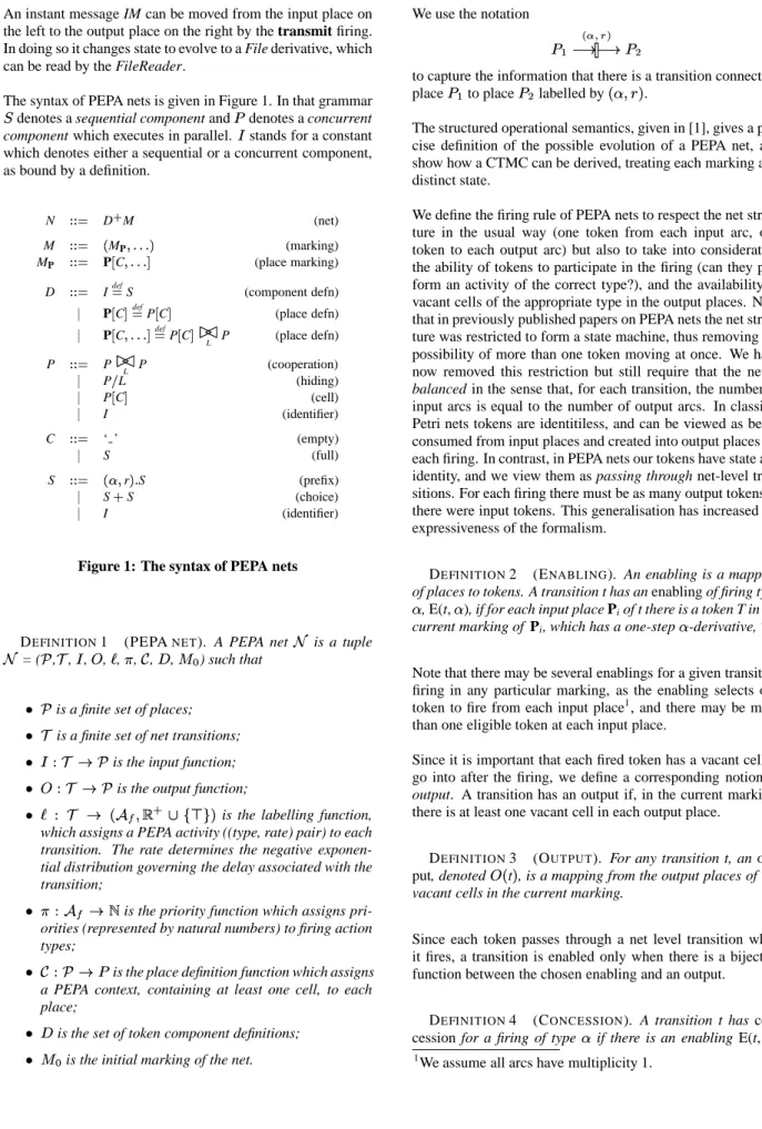
An instant message IM can be moved from the input place on the left to the output place on the right by the transmit firing. In doing so it changes state to evolve to a File derivative, which can be read by the FileReader.

The syntax of PEPA nets is given in Figure 1. In that grammar denotes a sequential component and denotes a concurrent

component which executes in parallel.stands for a constant

which denotes either a sequential or a concurrent component, as bound by a definition. N DM (net) M MP (marking) MP PC (place marking) D IdefS (component defn)

PC def PC (place defn) PC def PC L P (place defn) P P L P (cooperation) PL (hiding) PC (cell) I (identifier) C ‘ ’ (empty) S (full) S r S (prefix) SS (choice) I (identifier)

Figure 1: The syntax of PEPA nets

DEFINITION1 (PEPANET). A PEPA net is a tuple

= (,,,,,,,,) such that

is a finite set of places;

is a finite set of net transitions;

is the input function;

is the output function;

is the labelling function,

which assigns a PEPA activity ((type, rate) pair) to each transition. The rate determines the negative exponen-tial distribution governing the delay associated with the transition;

is the priority function which assigns pri-orities (represented by natural numbers) to firing action types;

is the place definition function which assigns

a PEPA context, containing at least one cell, to each place;

is the set of token component definitions;

is the initial marking of the net.

We use the notation

! " #

to capture the information that there is a transition connecting place to place#labelled by

$ %

.

The structured operational semantics, given in [1], gives a pre-cise definition of the possible evolution of a PEPA net, and show how a CTMC can be derived, treating each marking as a distinct state.

We define the firing rule of PEPA nets to respect the net struc-ture in the usual way (one token from each input arc, one token to each output arc) but also to take into consideration the ability of tokens to participate in the firing (can they per-form an activity of the correct type?), and the availability of vacant cells of the appropriate type in the output places. Note that in previously published papers on PEPA nets the net struc-ture was restricted to form a state machine, thus removing the possibility of more than one token moving at once. We have now removed this restriction but still require that the net is

balanced in the sense that, for each transition, the number of

input arcs is equal to the number of output arcs. In classical Petri nets tokens are identitiless, and can be viewed as being consumed from input places and created into output places for each firing. In contrast, in PEPA nets our tokens have state and identity, and we view them as passing through net-level tran-sitions. For each firing there must be as many output tokens as there were input tokens. This generalisation has increased the expressiveness of the formalism.

DEFINITION2 (ENABLING). An enabling is a mapping

of places to tokens. A transition t has an enabling of firing type

$

, E(t,

$

), if for each input place Piof t there is a token T in the

current marking of Pi, which has a one-step

$

-derivative, T&.

Note that there may be several enablings for a given transition firing in any particular marking, as the enabling selects one token to fire from each input place1, and there may be more than one eligible token at each input place.

Since it is important that each fired token has a vacant cell to go into after the firing, we define a corresponding notion of

output. A transition has an output if, in the current marking,

there is at least one vacant cell in each output place.

DEFINITION3 (OUTPUT). For any transition t, an out-put, denoted

t, is a mapping from the output places of t to

vacant cells in the current marking.

Since each token passes through a net level transition when it fires, a transition is enabled only when there is a bijective function between the chosen enabling and an output.

DEFINITION4 (CONCESSION). A transition t has con-cession for a firing of type

$

if there is an enabling E(t,

$

)

1

(4)

such that there is a bijective mapping from E(t, ) to an

output

t, which preserves the types of tokens.

As with classical Petri nets with priority, having concession identifies those transitions which could legally fire according to the net structure and the current marking. Those transitions which can fire are determined by the priorities.

DEFINITION5 (ENABLINGRULE). A transition t will be enabled for a firing of type

$

if there is no other transition of higher priority with concession in the current marking.

DEFINITION6 (FIRINGRULE). When a transition t fires

with type

$

on the basis of the enabling E(t,

$

), and concession

then for each (Pi, T,) in E(t, $

), T[T] is replaced by T[ ] in

the marking of Pi, and the current marking of each output

place is updated according to .

We assume that when there is more than one mapping from an enabling to an output, then they have equal probability and one is selected randomly. The rate of the enabled firing is determined using apparent rates, and the notion of bounded capacity, as usual for PEPA.

P 2 R[R] P 1 P[P] Q[Q] P 4 Q[Q’] R[−] P 3 R[−] P[−] t

Figure 2: PEPA net fragment to illustrate enabling

To illustrate the firing rules we consider the small PEPA net fragment shown in Figure 2. Here we assume that transition t has type

$

and that each of the tokens P, Q, and R has a one-step

$

-derivative (P&Q&and R&respectively). For the net

frag-ment shown there are two enablings:

P1P P2R and P1Q P2R

There are also two outputs:

P3P P4R and P3R P4R Note that P3P P3R is not an output.

Herehas concession because there is a bijective mapping

from P1P P2R to P3P P4R . Note that

the other potential mappings,

P1Q P2R to P3P P4R P1P P2R to P3R P4R and P1Q P2R to P3R P4R

are not valid because the types of tokens would not be pre-served.

If no other transitions of higher priority were enabled in the PEPA net this transition would fire, removing a P token from place P , and a R token from place P2and placing a P&token

in place P3and a R&token in place P4.

3. TRANSLATING PEPA NETS TO PEPA

In order to be able to exploit fully the existing suite of analy-sis tools for PEPA models we have defined a translation from PEPA nets to PEPA. In this section we describe the algorithm to do this in some detail. The algorithm is composed of a number of different steps which are described in turn in the following sections.

Before starting the translation, a preprocessing phase in nec-essary in order to rename firings that in the PEPA nets share the same input place and same action type. This is done by checking the arcs specification in the PEPA net file. For exam-ple, we need to make transformations of the arcs such as the following Pk ! " Pj and Pk ! " Pi Pk ! " Pj and Pk ! " Pi

and to store the triples (

$ $ % ) and ( $ $ #%#) in an array denoted by Fire.

Several data types and functions are used in the algorithm and are introduced below. In addition we use

, returning the

complete action type set of component

.

All stores all action types of the PEPA model

NumberSC counts occurrences of static components

Number

$

counts renamings of activity

$

as introduced by preprocessing

OccurSC stores repeated static components

Fire stores the triples from the preprocessing

TargetP stores triples P $ r where P is the

output place of the arc and

$ r

its label

Collect

$

stores the components which must synchronise

on the current action type

$

Extract

$

returns the original action type $

from the triple in Fire; Nil otherwise

sync

TiSCk

synchronisation set between token type

Tiand the static component SCk

returns the type of component

3.1 Step 1: Translating Static Components

This step concerns the translation of static components. We need to count the occurrences of static components within the places of the PEPA net and rename action types and deriva-tives of each occurrence of the static component to reflect its location. This allows us to avoid erroneous synchronisations since in a PEPA net synchronisation is possible only when the components are resident in the same place.

(5)

for each static component NumberSC ; OccurSC ;

for each place

if ( in then NumberSC NumberSC ; if (NumberSC then OccurSC ; for NumberSC make an instance of , renumber-ing activities and derivatives; //save all action types in All

AllAll

;

3.2 Step 2: Translating Cells

In this step we consider all the PEPA net places containing cells and we associate one component with each cell within a place. Each cell definition is built by considering the input and output arcs to the place itself, with respect to the type of the token which may occupy the cell. Moreover, each cell can be in two states: empty, denoted by a subscript 0 in its derivative, and full denoted by a subscript 1. Firing a token into the place changes the state of the cell from empty to full. Firing a token out of the cell changes its state from full to empty. This allows us to prevent a token from moving to a place where all of the cells are already full.

for each token type and place

for each cell

in

create a component Cell

;

for each input arc ! " such that $ AllAll $ ;

//avoiding redundant activities

Cell Cell $ r Cell ;

for each output arc ! r such that $ AllAll $ ; Cell Cell $ r Cell ;

3.3 Step 3: Translating Tokens

Token definitions need to be revised according to their dynamic behaviour. Two aspects are taken into account: the movement of a token into a new place after a firing and its interaction with static components within a PEPA net place. Again, in order to avoid erroneous synchronisations, we need to cre-ate new names for action types and derivatives. This is done when two or more net transitions have the same label and when tokens synchronise with static components which appear sev-eral times in the net. Recall that in Step 1 the action types

and the derivatives of each occurrence of the static component were renamed. Therefore here we need to copy the derivatives of the token where the synchronising action type appears and we do this for each renaming of the synchronising action.

for each token type Ti

//movement of the token in the net

for each action type

$ Ti Number $ ; TargetP ;

for each arc actionr $ Extract action; if ( $ $ ) then Number $ Number $ ; TargetP TargetP ; if (Number $ ) then r rNumber $ ;

for each distinct place in TargetP

add the corresponding activity

actionr

in TargetP

followed by a new com-ponent identifier

;

duplicate the sequential component

resulting from the execution of action

$ in Ti, replacing with ;

else make a copy of the current derivative of Ti;

//interaction of token and static components

for each place

if (Tiin ) then

for each static component SCkin OccurSC

for each action type

$ sync TiSCk for NumberSC

duplicate the derivatives where

$

appears in Tifor each

renam-ing of

$

during the translation of the static component SCk;

//representing the initial marking

for each occurrence of at in make an instance of , renumbering

activities and derivatives.

3.4 Step 4: Building the System Equation

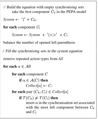
The “system equation” of a PEPA model forms a parallel com-position of the process components which have defining equa-tions. Several copies of each component might be required and any instance of a process definition can be configured by the use of a synchronisation set which forces it to synchronise with one or more of the other processes. We build the system equation for the PEPA model generated from the input PEPA net by putting in parallel all the components generated in the previous steps. Then we force them to synchronise on com-mon action types.

(6)

//Build the equation with empty synchronising sets take the first component in the PEPA model

System & & ;

for each component

SystemSystem & &

balance the number of opened left parenthesis //Fill the synchronising sets in the system equation

remove repeated action types from All

for each

$

for each component

if $ then Collect $ ;

for each pair

Collect $ if then insert $

in the synchronisation set associated with the most left component between

and

3.5 Properties of the translation

PEPA stochastic process algebra models have no notion of context, nor any capacity to move components from one con-text to another, and therefore cannot express the concept of dynamically varying communication structure. The task per-formed by the compilation of a PEPA net described above has been to remove all of the mobility from the PEPA net by making components’ behaviour depend on location. This is achieved by expanding the definition of the tokens of the net replicating local state behaviours and customising these for each cell which the token may visit.

The compilation from a PEPA net to a PEPA model is analo-gous to the preprocessing of a coloured Petri net to transform it into an uncoloured net for analysis purposes. In the worst case—when there is only a single class of token, all tokens can travel to all of the places of the net, and the net has no static components—the resulting PEPA model istimes larger than

the input PEPA net, whereis the number of cells in the net.

Thus there is no exponential increase in the size of the repre-sentation of the model here and the compilation procedure runs in a time proportional to the size of the model, not the size of the state space which it would generate when fired against the operational semantics of the language.

The correctness of the translation from the input PEPA net to the resulting PEPA model can be stated formally thus. When evaluated against the operational semantics of the languages the two models generate labelled transition systems (LTS) for the models. These LTS contain information about the activities performed in the model by including action types in labels. If these occurrences of action types are removed then isomorphic CTMCs are obtained for the input PEPA net and its translation. This is the sense in which the output PEPA model is a correct translation of the input PEPA net.

4. EXAMPLE: MOBILE AGENTS

We present a small example to reinforce the reader’s under-standing of the translation algorithm. In this example a mobile software agent visits three sites. It interacts with static soft-ware components at these sites and has two kinds of interac-tions. When visiting a site where a network probe is present it interrogates the probe for the data which it has gathered on recent patterns of network traffic. When it returns to the cen-tral co-ordinating site it dumps the data which it has harvested to the master probe. The master probe analyses the data.

4.1 The PEPA net Model

The structure of the application is as represented by the PEPA net in Figure 3. This marking of the net shows the mobile agent resident at the central co-ordinating site. Recall that as a memory aid, in both the net and the PEPA token definitions, we print in bold the names of those activities which can cause a firing of the net. In this example the activities which can cause a firing of the net are go and return.

T1 T2 T3 T4 go go return return P1 P2 Agent P3

Figure 3: A simple mobile agent system

Formally, we define the places of the net as shown in the PEPA context definitions below.

P1Agent def AgentAgent interrogate Probe P2Agent def AgentAgent dump Master P3Agent def AgentAgent interrogate Probe

The behaviour of the components is given by the following PEPA definitions. Agent def go Agent & Agent& def interrogateri Agent && Agent&& def return Agent &&& Agent&&& def dumprd Agent Master def dump Master & Master& def analysera Master Probe def monitorrm Probe interrogate Probe

The initial marking of the net has one Agent token in place P2

and no other tokens:

Agent interrogate Probe AgentAgent dump Master Agent interrogate Probe

(7)

4.2 Translation into PEPA

The example has two static components Master and Probe. As the latter appears twice in the PEPA net model (in places

P1 and P3), the application of the algorithm generates two

instantiations of this component Probe1and Probe2. Thus in

the PEPA model we have:

Master def dump Master & Master& def analysera Master Probe1 def monitor1rm Probe1 interrogate1 Probe1 Probe2 def monitor2rm Probe2 interrogate2 Probe2

As each place contains just one cell, the translation algorithm will generate three new components which we will denote by

Cellj 0, where the subscript j = 1, 2 or 3 specifies that the cell

resides at place P1, P2or P3. The suffix which follows j takes

only the values zero or one and is used to record whether the cell is empty or full2_.

Firings and transitions are no longer distinguished because there is only one class of activities in PEPA and so we no longer embolden the names go and return.

Cell10 def go Cell11 Cell11 def return Cell10 Cell20 def return Cell21 return# Cell21 Cell21 def go Cell20 # Cell20 Cell30 def go# Cell31 Cell31 def return# Cell30

Component Agent is the token in the net and its definition is modified to take into account its complete dynamic behaviour in the net. Agent def go Agent go# Agent Agent def interrogate1ri Agent Agent def interrogate2ri Agent Agent def return Agent Agent def return# Agent Agent def dumprd Agent

The PEPA system equation forms a parallel composition of instances of the above components and requires them to syn-chronise on their common actions. The system equation in this case is as follows: System def Cell10 K1 Probe K2 Agent K3 Cell21 K4 Master K5 Probe1 K6 Cell30 where K1= go1, return1, K2= interrogate1, K3= go1,

return1, go2, return2, dump, interrogate2, K4=

go2, K5=

K6=.

2

Note that since there is only one token type in this PEPA net we omit the corresponding subscript.

5. IMPLEMENTATION

We have implemented our translation from PEPA nets to PEPA as an extension to our existing tool, The PEPA Workbench for PEPA Nets, ML Edition. This is a modular research version of the PEPA Workbench for experimentation and extension so it is well-suited to adding modules such as the PEPA net com-piler.

The workbench front end which consists of the PEPA net parser and syntax tree builder required no changes from their use as components of the PEPA Workbench. Similarly, the static analyser for PEPA nets was unchanged. The new components added by the compiler make use of this front end and then pro-vide other functions for traversing the abstract syntax tree of the PEPA net and inferring derived synchronisation sets from the union of sets which are stored throughout the tree. Simi-larly, token flows were inferred for the components which flow around the net. Additionally, new names were coined for spe-cialisations of activities within cells. Finally, a PEPA “system equation” is generated which composes the images of tokens, cells and static components using the appropriate inferred syn-chronisation sets.

We have found the implementation of the compiler to be very efficient in practice. The PEPA net compiler does not unfold the global state space of the model. Instead it uses the compo-sitional nature of the PEPA net when constructing an equiva-lent PEPA model. In this way, the compilation is performed in linear time, with respect to the size of the original PEPA net description.

6. PLATFORM SUPPORT FOR PEPA

As mentioned earlier, the objective of the translation from the PEPA nets modelling language into the PEPA stochastic pro-cess algebra is to allow the PEPA net modeller to exploit the existing suite of tools which support PEPA. In this section we give a brief overview of these tools. We will use these tools in processing our case study example in Section 7 so we provide an explanation of these tools here before we use them later. We see the provision of tool support for modelling languages as being analogous to providing tools for programming lan-guages. A software development kit typically provides a range of tools (compilers, debuggers, profilers, perhaps even model checkers) which perform various types of analysis or conver-sion on the program. Similarly in providing platform sup-port for PEPA and PEPA nets we provide this through a mod-elling kit containing solvers, passage-time analysers, model-checkers and other tools.

The analysis of a PEPA model proceeds by deriving its under-lying Markov chain and solving this to find the long-run prob-ability of the states of the chain. The states of the chain are in one-to-one correspondence with the states of the deriva-tion graph of a PEPA process as specified by the operaderiva-tional semantics of the language so information about the long-run behaviour of the CTMC translates directly to information about the PEPA model from which it was derived.

The PEPA Workbench [3] generates the CTMC correspond-ing to any given PEPA model. The Workbench is available in

(8)

two editions (principally implemented in ML and Java respec-tively), connected to a variety of solvers for the CTMC. Addi-tionally, in 1999 Clark implemented some additional PEPA tools such as the PEPAroni simulator in Pizza [4], an extension of Java. This was later re-implemented in the Java version of the Workbench [5].

The PEPA Workbench is available for download from the PEPA Web site located athttp://www.dcs.ed.ac.uk/pepa/

together with documentation, example models and copies of papers on PEPA and PEPA nets.

6.1 Analysis Tools

Generating the underlying CTMC, and finding its steady state probability vector is rarely, if ever, the objective of PEPA or PEPA net modelling. Formal tool support for querying per-formance models is an area which has received little attention until recently, despite its practical importance.

At the most basic level the modeller wishes to construct a

reward structure over the state space of the CTMC, to be used

in conjunction with the steady state probability vector to derive performance measures. For steady state measures the reward structure is a vector recording a reward for each state, although for many states the reward value will be zero. Thus the prob-lem becomes one of identifying the appropriate set of states to attach a non-zero reward to. Clearly, when the CTMC arises from a stochastic process algebra model we prefer to charac-terise the state at the process algebra level. PEPA analysis tools have been developed which tackle this problem in two distinct ways.

6.1.1 The PEPA State Finder

The PEPA State Finder identifies subsets of states using regu-lar expression pattern matching, applied to the table of PEPA expressions which make up the state of the model. Recall that there is a one-to-one correspondence between the syntac-tic forms of the PEPA process as it evolves and the states of the CTMC. The Workbench maintains a table recording this cor-respondence, and using regular expression pattern matching the PEPA State Finder is able to extract the states of inter-est. For example, it is possible to use an expression such

*|(next,r).*to return the state numbers of all the states in which the second component enables a (next, r) activity. This could then be used to construct a reward structure suit-able for calculating the throughput of next in the second com-ponent: the value r is placed in the reward vector at each posi-tion corresponding to a (numerical) state found by the PEPA State Finder.

6.1.2 PML

A more sophisticated means of specifying rewards is described in Clark’s PhD thesis [6], and developed around the stochas-tic logic PML . Inspired by the probabilisstochas-tic model logic of Laren and Skou, PML [7], PML is able to differentiate PEPA terms which perform the same activities but at different rates. The key to this is a modification to Hennessy-Milner logic in which the diamond operator becomes decorated with a rate. The semantics of an expression in the logic is a subset of states, and thus logical expressions may be used, in conjunction with

a value, to specify a reward structure. Clark extended the ML edition of the PEPA Workbench to include support for PML and associated reward structures [6].

6.1.3 CSL

More recently the CSL logic (Continuous Stochastic Logic) [8] has gained some acceptance as a suitable vehicle for express-ing performance and performability measures which can be model checked on a CTMC. Unlike the approach of PML , where the logic formula is used to distinguish a subset of states (those satisfying the formula), a CSL formula expresses an assertion about the performance measures of a model which can then be checked to see whether it is true or not. Thus this offers an alternative approach to using logics to assist in per-formance analysis.

6.2 Interoperation with other tools

In addition to developing tools specific to PEPA, when possi-ble we connect the PEPA language to existing tools for perfor-mance modelling.

6.2.1 PEPA and M¨obius

The Möbius modelling framework [9] is a multi-formalism and multi-paradigm modelling tool, and as such provided an excellent tool to integrate PEPA into [10]. Integration in this case involved not only building PEPA support into Möbius but also incorporating Möbius features into the version of PEPA which was implemented in Möbius. The reason for this was that it then became possible to share variables between com-ponents modelled in PEPA and comcom-ponents implemented in another Möbius formalism, such as SANs.

Building support for PEPA directly in another tool has the advantage that the language is supported efficiently, without additional overheads imposed by translation from one repre-sentation into another. However, it has the implementation cost that the implementor must be familiar not only with the concepts of the host tool but also with their representation in data structures and algorithms. Such tight integration is not always cost-effective or necessarily desirable.

6.2.2 PEPA and PRISM

For our subsequent integration work we used a lighter-weight, component-based method involving a relatively loose coupling between the language and the host solver. This was adopted when a binding for the PEPA language in the PRISM [11] probabilistic model checker was developed. In PRISM analy-sis of CTMCs is performance through model checking speci-fications in the probabilistic temporal logic CSL.

In order to define and analyse a model, PRISM requires two input files: a description of the system under investigation and a set of properties to be checked against it. The description of the system is given in a reactive module language. To integrate PEPA, a PEPA compiler was adapted to generate its output in the form of this language. Additionally, the model checker itself was extended to support PEPA’s combinators (parallel and hiding).

(9)

This method of working with PEPA models requires a signif-icant degree of expertise on the part of the modeller, because errors in evaluation can occur in the tool chain right from the PEPA parser through PEPA-to-PRISM and PRISM down to CUDD [12], the BDD library which provides MTBDD data structures and algorithms to PRISM. Even if errors do not occur in translation still to achieve the best performance from the solver it is necessary to know how to configure both PRISM and CUDD which means that this method is best suited to experienced modellers only.

The PRISM tool is available for download from www.cs. bham.ac.uk/˜dxp/prism/.

6.2.3 PEPA, IPC and Dnamaca

A recent development in the PEPA tools is Bradley’sipc(The Imperial PEPA Compiler) [13]. Theipctool translates an input PEPA model into the Petri net notation provided by Knotten-belt’s Dnamaca tool [14]. Theipctool supports the PEPA lan-guage comprehensively. Apparent rates are supported, as are anonymous components. These are two advantages over the PEPA-to-PRISM compiler, and a richer class of PEPA models can therefore be analysed byipc/Dnamaca as a result. In one other important respect, ipcprovides more compre-hensive PEPA support than comparable tools because it also translates PML formulae into the Dnamaca specification lan-guage. The Dnamaca specification language is a classical Petri net logic allowing specification formulae to quantify the num-ber of tokens in the places of the net and thereby identify states and sets of states within the reachable state space of the model. Viaipc, the unique solution capabilities of Dnamaca become available and because of this it is possible to perform efficient passage time analysis over PEPA models.

Theipccompiler is available for download fromwww.doc. ic.ac.uk/ipc.

7. EXAMPLE: SECURE WEB SERVICE

In this section we present a PEPA net model of an exam-ple taken from the field of Web Services, a relatively new Web programming paradigm which provides standard inter-faces and communication protocols for integrating Web-based distributed applications.

Web services allow different applications from different sources to communicate and interoperate. Many practitioners believe that they will become a key component of many organization’s future business-integration initiatives. Security issues need to be considered carefully because the integration of applications that communicate over a network could reveal sensitive infor-mation to unknown parties.

Web services interfaces are defined, described and discovered by means of XML—the eXtensible Markup Language—and therefore they are not tied to any single operating system or programming language. XML is used to tag the data which are exchanged between applications via SOAP (Simple Object Access Protocol) messages, XML-based messages which may

be transported using a variety of Internet protocols, including SMTP, MIME, and HTTP.

The available services are described using WSDL (the Web Services Description Language), an XML-formatted language, and they are made available thanks to UDDI (the Universal Description, Discovery and Integration format), a Web-based distributed directory that lists the available services, similar to a traditional phone book’s yellow and white pages.

Our example is a model of a mobile object system where a client sends SOAP message objects to a remote Web service. Our scenario is that a financial tycoon is sending requests for stocks and share price information to a remote Web service which provides this information. These requests for informa-tion are encrypted. An eavesdropper could make use of the information in the messages if they were sent as clear text. The Web service itself is protected by a firewall.

7.1 The token type

The tokens exchanged in the system are SOAP messages in various formats. These may either be sent across the network as clear text or encrypted to preserve their contents. A SOAP message may be parsed to build an in-memory data structure which can be read and modified as needed. This data structure is a DOM tree (a Document Object Model tree).

SoapMessage def sendclrrsc SentClearMessage encryptre EncryptedMsg parserp DOMtree SentClearMessage def copyClear SoapMessage

The rate at which information is copied across the network is specified not in this component but at the upper PEPA net level. The description of this component leaves unspecified (

) the rates at which these actions are performed, allowing the cooperating partner in the synchronisation to determine these rates. All such unspecified rates must be synchronised with specified ones in the final model. Frequently, synchronisations are between one active partner and one passive partner. Encrypted messages can be decrypted to recover their initial contents or sent across the network in encrypted form.

EncryptedMsg def decryptrd SoapMessage sendencrse SentEncMessage SentEncMessage def copyEncrypted EncryptedMsg

In both cases, we model the transmission of a SOAP mes-sage as a two-phase process, separating the cost of making the decision to send (sendclr, sendenc) from the cost of copying

the bytes across the network (copyClear, copyEncrypted). DOM trees may be read or modified. As an in-memory data structure they first must be serialised (using the export activity) if they are to be sent across the network.

DOMtree def readrr DOMtree modifyrm DOMtree exportrx SoapMessage

(10)

7.2 Static components

SOAP message tokens of various forms are exchanged between the places of the net. Static components at these places interact with the tokens. On the client side is the user, making requests of the remote Web Service. The user encrypts requests before they are sent and decrypts replies when they are received.

User def Encrypt

Decrypt Encrypt def encrypt sendenc User Decrypt def decrypt parse read Request Request def modify export User

Running on the firewall is a gatekeeper process which per-forms three distinct functions: decrypting user requests, bounc-ing flawed requests and encryptbounc-ing replies from the server. The gatekeeper receives requests from the user and decrypts them. The decrypted message might be a well-formed request, in which case it is forwarded to the server. Alternatively it might be in an invalid format, request a non-existent service, or have suspicious attachments. In this case it is bounced back to the user with a diagnostic error message attached. This assign-ment of responsibilities means that the load on the server is reduced.

All of the communication with the user is sent in encrypted format. Behind the firewall the messages are exchanged in the clear. Thus sendencalways sends to the user and sendclralways

sends to the server.

GateKeeper def FilterIn

Bounce FilterOut FilterIn def decrypt sendclr GateKeeper Bounce def decrypt FilterOut FilterOut def encrypt sendenc GateKeeper

Behind the firewall the share price Web service runs on the server. Its life cycle is parsing, reading, modifying, serialising and returning requests.

WebServicedef parse read modify export sendclr WebService

7.3 The PEPA net

The PEPA net of the system sites the above static components at places of the net and specifies the communication between different places of the net by naming the transitions which must be fired for tokens to move from place to place. The

User is operating the client machine, the GateKeeper process

runs on the firewall, the WebService on the server behind the firewall. Client side User L SoapMessage SoapMessage copyEncryptedrce copyEncryptedrce GateKeeper L EncryptedMsg copyClearrcc copyClearrcc WebService L SoapMessage Server side

The synchronisation set used at each place, L, is

decrypt, sendclr, parse, read, modify, export, encrypt, sendenc.

7.4 Model analysis

We analysed our secure Web service model using the PEPA Workbench for PEPA nets and the PRISM model checker, mak-ing use of our PEPA net compiler tool to compile the net into a PEPA model which is accepted by PRISM.

7.4.1 Using the PEPA Workbench for PEPA nets

The PEPA Workbench for PEPA nets implements the seman-tics of the PEPA nets language directly and generates a CTMC suitable for performance analysis.

In the analysis of our example using the PEPA Workbench we calculated the utilisation of the Web service as two quanti-ties varied. The first was the probability (bounceProb) that user requests to use the Web service would be bounced by the gatekeeper process (for whatever reason). We varied this between 0.05 (there is a low probability that requests will be bounced) and 1.0 (requests messages are always bounced, and do not reach the server). The second parameter which we var-ied was the strength of the encryption used to encrypt mes-sages. This variation is captured by an increase in the overhead associated with encryption and decryption (encOver). We plot-ted this for strong encryption taking in the range ten times longer to compute to ninety times longer.

0.2 0.4 0.6 0.8 1 bounceProb 20 40 60 80 encOver 0 0.02 0.04 0.06 utilProb

As expected, the utilisation of the Web service is seen to be lowest when the strongest form of encryption is used (because this delays only the user and the gatekeeper) and when the probability of bouncing messages is highest (in that case they never reach the server).

7.4.2 Using the PEPA nets compiler

The PEPA nets Compiler is a component of the PEPA Work-bench for PEPA nets. It compiles the secure Web service example from a PEPA net into an equivalent PEPA process algebra model in 0.02 seconds on a 1.6GHz Pentium IV pro-cessor machine with 256Mb of memory. The GNU time

command version 1.7 was used to obtain this timing informa-tion. The time reported is elapsed real (wall clock) time used by the process. This compilation facilitates further analysis with tools which support PEPA.

7.4.3 Model-checking using PRISM

We used PRISM to model check a range of CSL formulae over the PEPA model generated by the PEPA net compiler. One formula which we checked was “with probability at least 0.5,

(11)

the web service begins processing its first request within t time units”. This is expressed in CSL as follows:

P 0.5true Ut WebService read WebService &

This is a typical CSL formula, combining time, probability and a path through the system evolution. We checked this for-mula with the time parameter, t, taking values between 1.0 and 100,000.0 time units. Model-checking formulae of this type on a 1.6GHz Pentium IV processor machine with 256Mb of memory typically requires an average of 0.275 seconds of compute time, as reported by PRISM. These times are mea-sured in the PRISM implementation using Java’s native method System.currentTimeMillis(). The formula above is satisfied for all states of the secure Web Service model for values of

t=250 time units and higher.

7.4.4 Passage-time analysis using

ipc

/DNAmaca

Some questions which we would like to ask of a performance model are not readily answered from the computation of the steady-state probability distribution of the model, nor are they answered by model-checking time-bounded probabilistic for-mulae against the model. Queries such as those involving responsiveness of the system under workload—“does the sys-tem respond within 5 seconds 90% of the time?”—are instead answered by reference to passage-time quantiles.

To undertake analysis of this form we use the Imperial PEPA Compiler (ipcv0.91a 230603, James Clerk Maxwell Release) together with the DNAmaca analyser for Markov and semi-Markov chains (Hydra release). This tool chain has previously been used to analyse PEPA models [15] but this is the first application of these tools to a PEPA net.

The plot below shows the cumulative density function for the passage from the user initiating a web service request on the client side to the initiated computation being completed at the server side. 0.1 0.2 0.3 0.4 0.5 0.6 0.7 0.8 0.9 1 0 0.5 1 1.5 2 2.5 3 3.5 4 4.5 5 Pr Time in seconds CDF plot of Web service model

In order to effect the passage-time analysis of this model we used the method of stochastic probes [16] whereby additional stochastic process algebra components are generated to probe the system to observe the specified start events and end events. The resulting extended PEPA model is then compiled byipc

into a DNAmaca model.

Specifically in this case the PEPA actions which we probed were sendencat the Client place and sendclrat the Server place

in the net. The PEPA net compiler distinguishes these in the

resulting PEPA stochastic process algebra model so that we can be sure that we are probing these activities and not the

sendencand sendclractivities which occur at the Firewall place

in the PEPA net.

8. CONCLUSIONS

Building performance models of realistic real-world systems is an activity which requires careful attention to detail in order to model correctly the intended behaviour of the system. Pro-ceeding with care during this part of the modelling process is a wise investment of effort. If the initial performance model contains errors then all of the computational expense incurred in solving the model and all of the intellectual effort invested in the analysis and interpretation of the results obtained would at best be wasted. In general interpreting a model with errors could lead to making flawed economic or strategic decisions based on erroneous conclusions made from erroneous results. For this reason we consider it important to work with struc-tured, high-level modelling languages which directly support the concepts and idioms of the application domain, such as code mobility. In this paper we have shown how a mobile code modelling language, PEPA nets, can be mapped into another language, the stochastic process algebra PEPA, where mobil-ity is not directly expressible in the language and there is no notion of physically or logically separated locations being a barrier to communication.

Our translation from PEPA nets to PEPA has enough subtleties that it was worthwhile to implement it in a software tool to prevent making mistakes that could easily be made if applying the method by hand. We extended our existing workbench for PEPA nets for this purpose, building in a compiler from PEPA nets to PEPA. We applied this to a case study of modelling a secure Web Service. We analysed the resulting performance model for steady-state behaviour, transient behaviour exposed by CSL model-checking, and responsiveness quantified by the computation of passage-time quantiles.

Acknowledgements

Stephen Gilmore, Jane Hillston and Le¨ıla Kloul are supported by the Design Environments for Global ApplicationS project (DEGAS) IST-2001-32072 funded by the Future and Emerg-ing Technologies Proactive Initiative on Global ComputEmerg-ing. Their collaboration with Ribaudo was supported by the Dipar-timento di Informatica, Universit`a degli Studi di Torino. Marina Ribaudo is supported by the FIRB project WEBMINDS (Wide-scalE, Broadband, MIddleware for Network Distributed Ser-vices).

The authors have benefitted from their collaboration with Linda Brodo and Corrado Priami on mapping PEPA nets into the stochastic-calculus and Stochastic CCS. The PEPA to PRISM

compiler was developed in collaboration with Gethin Norman and Dave Parker of The University of Birmingham. Jeremy Bradley advised on the use of stochastic probes and the use of the Hydra release of DNAmaca.

The anonymous referees provided many very helpful com-ments which allowed us to improve the presentation of the paper in this revision.

(12)

9. REFERENCES

[1] S. Gilmore, J. Hillston, M. Ribaudo, and L. Kloul. PEPA nets: A structured performance modelling formalism.

Performance Evaluation, 54(2):79–104, October 2003.

[2] J. Hillston. A Compositional Approach to Performance

Modelling. Cambridge University Press, 1996.

[3] S. Gilmore and J. Hillston. The PEPA Workbench: A Tool to Support a Process Algebra-based Approach to Performance Modelling. In Proceedings of the Seventh

International Conference on Modelling Techniques and Tools for Computer Performance Evaluation, number

794 in Lecture Notes in Computer Science, pages 353–368, Vienna, May 1994. Springer-Verlag. [4] M. Odersky and P. Wadler. Pizza into Java: Translating

theory into practice. In Proceedings of the 24th ACM

Symposium on Principles of Programming Languages (POPL’97), Paris, France, pages 146–159. ACM Press,

New York (NY), USA, 1997.

[5] Fotis Stathopoulos. Enhancing the PEPA Workbench with simulation and experimentation facilities. Master’s thesis, School of Computer Science, Division of Informatics, The University of Edinburgh, 2001. [6] G. Clark. Techniques for the Construction and Analysis

of Algebraic Performance Models. PhD thesis, The

University of Edinburgh, 2000.

[7] Kim Guldstrand Larsen and Arne Skou. Bisimulation through probabilistic testing. Information and

Computation, 94(1):1–28, 1991.

[8] A. Aziz, K. Sanwal, V. Singhal, and R. Brayton. Verifying continuous time Markov chains. In

Computer-Aided Verification, volume 1102 of LNCS,

pages 169–276. Springer-Verlag, 1996. [9] G. Clark, T. Courtney, D. Daly, D. Deavours,

S. Derisavi, J. M. Doyle, W. H. Sanders, and P. Webster. The M¨obius modeling tool. In Proceedings of the 9th

International Workshop on Petri Nets and Performance Models, pages 241–250, Aachen, Germany, September

2001.

[10] G. Clark and W.H. Sanders. Implementing a stochastic process algebra within the M¨obius modeling framework. In L. de Alfaro and S. Gilmore, editors, Proceedings of

the first joint PAPM-PROBMIV Workshop, volume 2165

of Lecture Notes in Computer Science, pages 200–215, Aachen, Germany, September 2001. Springer-Verlag. [11] M. Kwiatkowska, G. Norman, and D. Parker.

Probabilistic symbolic model checking with PRISM: A hybrid approach. In J.-P. Katoen and P. Stevens, editors,

Proc. 8th International Conference on Tools and Algorithms for the Construction and Analysis of Systems (TACAS’02), volume 2280 of LNCS, pages 52–66.

Springer, April 2002.

[12] F. Somenzi. CUDD: CU Decision Diagram Package. Department of Electrical and Computer Engineering, University of Colorado at Boulder, February 2001.

[13] J.T. Bradley, N.J. Dingle, S.T. Gilmore, and W.J. Knottenbelt. Derivation of passage-time densities in PEPA models using IPC: The Imperial PEPA Compiler. In G Kotsis, editor, Proceedings of the 11th IEEE/ACM

International Symposium on Modeling, Analysis and Simulation of Computer and Telecommunications Systems, pages 344–351, University of Central Florida,

October 2003. IEEE Computer Society Press. [14] W.J. Knottenbelt. Generalised Markovian analysis of

timed transition systems. Master’s thesis, University of Cape Town, 1996.

[15] J.T. Bradley, N.J. Dingle, S.T. Gilmore, and W.J. Knottenbelt. Extracting passage times from PEPA models with the HYDRA tool: A case study. In S. Jarvis, editor, Proceedings of the Nineteenth annual

UK Performance Engineering Workshop, pages 79–90,

University of Warwick, July 2003.

[16] A. Argent-Katwala, J. T. Bradley, and N. J. Dingle. Expressing performance requirements using regular expressions to specify stochastic probes over process algebra models. In Proceedings of the 4th International

Workshop on Software and Performance, 2004. This