Does anticipation of government spending matter? The role of (non-)defense spending

Bonn Econ Discussion Papers

Bonn Graduate School of Economics Department of Economics

University of Bonn Kaiserstrasse 1 Discussion Paper 12/2010

Does anticipation of government spending matter?

The role of (non-)defense spending

by

Jörn Tenhofen and Guntram B. Wolff

Financial support by the

DeutscheForschungsgemeinschaft(DFG)

through the

BonnGraduateSchoolofEconomics(BGSE)

is gratefully acknowledged.

Does anticipation of government spending

matter? The role of (non-)defense spending

J¨orn Tenhofen

and Guntram B. Wolff

Bonn and Frankfurt, May 20, 2010

Abstract

We investigate the effects of government expenditure on private con-sumption when the private sector anticipates the fiscal shocks. In order to capture anticipation of fiscal policy, we develop a new method based on a structural vector autoregression (SVAR). By simulating data from a theoretical model featuring (imperfect) fiscal foresight, we demon-strate the ability of our new approach to correctly capture macroeco-nomic dynamics. We take advantage of the flexibility of our econo-metric approach and study those subcomponents of total government spending, which have different macroeconomic effects according to eco-nomic theory. Using post-WWII US data, we find that when taking into account anticipation, private consumption significantly decreases in response to a defense expenditure shock, whereas when considering shocks to non-defense spending, consumption increases significantly. A standard SVAR does not produce clear consumption responses, high-lighting the importance of anticipation. Our results thus reconcile the different findings of the narrative and SVAR approaches to the study of fiscal policy effects.

∗_{University of Bonn, email: joern.tenhofen@uni-bonn.de}

∗∗_{Deutsche Bundesbank, University of Pittsburgh, email: guntram.wolff@gmx.de}

††_{We thank Benjamin Born, J¨org Breitung, Sandra Eickmeier, Zeno Enders, Michael}

Evers, Monika Merz, Gernot M¨uller, Johannes Pfeifer, Valerie Ramey, Stephanie Schmitt-Groh´e, Harald Uhlig, Mart´ın Uribe, participants of the Bundesbank economic seminar, of the Bonn-Frankfurt Workshop ”Topics in Time Series Econometrics,” of the University of Pittsburgh economics seminar, of the IMF seminar, of the University of Bonn Macro Workshop, and of the 2nd Amsterdam-Bonn Workshop in Econometrics for many helpful comments. The opinions expressed in this paper do not necessarily represent the views of the Deutsche Bundesbank or its staff.

1

Introduction

The empirical literature on the effects of fiscal policy on the macroeconomy is inconclusive. It can broadly be divided into two strands according to the identi-fication approach. On the one hand, fiscal policy events are identified with the narrative approach employing dummy variables that indicate large increases in government expenditure related to wars.1

These foreign policy events are assumed to be exogenous to the state of the economy and can therefore be used to identify the effects of fiscal policy. This line of research typically finds that in response to such a shock to government spending, GDP increases whereas private consumption and real wages fall (Ramey and Shapiro 1998, Edelberg, Eichenbaum, and Fisher 1999, Burnside, Eichenbaum, and Fisher 2004). On the other hand, structural vector autoregressions (SVARs) usually achieve identification by assuming that government spending is predetermined within the quarter and government revenue does not respond to macroeconomic de-velopments in the same quarter except for exogenous automatic stabilizers (Blanchard and Perotti 2002). This strand of the literature finds that private consumption, similar to GDP, usually increases after a shock to government spending. Those results have been confirmed and extended in the papers by Perotti (2005, 2008), for example.2

These contrasting empirical findings have important implications for our view of the macroeconomy. Standard macroeconomic models focusing on fiscal policy such as the neoclassical model of Baxter and King (1993) but also most New-Keynesian variants (for example, Linnemann and Schabert (2003)) have an unambiguous prediction concerning the response of private consumption to a shock to government spending. Whereas output is expected to increase in response to such a shock, consumption should fall. The central reason for the latter dynamic response in those models is that government expenditure (fi-nanced by lump-sum taxes) constitute a withdrawal of resources from the econ-omy, which in turn do not substitute or complement private consumption nor

1_{The narrative approach goes back to Romer and Romer (1989) in the area of monetary}

policy. A recent paper by Romer and Romer (2009) employs the narrative approach for tax changes.

2_{More empirical evidence with respect to European countries is provided by Biau and}

Girard (2005) for France, Giordano, Momigliano, Neri, and Perotti (2007) for Italy, de Castro and de Cos (2008) for Spain, and Tenhofen, Wolff, and Heppke-Falk (2010) for Germany. A different identification procedure was proposed by Fat´as and Mihov (2001) and Mountford and Uhlig (2009), who also document a positive consumption response.

contribute to productivity. The resulting adverse wealth effect drives the nega-tive consumption response. In contrast, Gal´ı, L´opez-Salido, and Vall´es (2007) construct a New-Keynesian model with a positive consumption response, in order to reconcile current business cycle models with the empirical findings of the SVAR literature. Gal´ı, L´opez-Salido, and Vall´es (2007) make clear, how-ever, that many very special conditions have to be fulfilled for the model to be able to generate a positive response of private consumption. In particu-lar, sticky prices and ”rule-of-thumb” consumers drive the result.3

Empirical findings therefore shape our modeling and understanding of the economy. Un-fortunately, however, the different methods employed do not yield consistent results.

In an important contribution, Ramey (2009) aims at explaining the dif-ference between the results of the two empirical approaches. She argues that VAR techniques miss the fact, that major changes in government spending, such as expenditure related to wars, are usually anticipated. Within a stan-dard model, it is easy to show, that missing the point of anticipation will result in a positive response of consumption to a shock to government spending, as consumption following the initial drop increases with investment. In support of her hypothesis that shocks are indeed anticipated, Ramey (2009) documents that the war dummy shocks Granger-cause the VAR shocks, but not vice versa. These problems fit into the more general discussion on when it is pos-sible to relate the innovations recovered by a VAR to the shocks of a par-ticular economic model. Early contributions in this regard are Hansen and Sargent (1980, 1991), Townsend (1983), Quah (1990), and Lippi and Reichlin (1993, 1994), with a recent reminder of these problems to the profession in Fern´andez-Villaverde, Rubio-Ram´ırez, Sargent, and Watson (2007). An appli-cation of these insights to fiscal policy anticipation, in particular concerning tax changes, with a thorough discussion of the related issues can be found in Leeper, Walker, and Yang (2009). This literature centers on the fundamental problem that in certain setups the information sets of the private agents and the econometrician are misaligned. In the case of fiscal policy anticipation, this means that private agents in addition to the variables observed by the econometrician know about the fiscal policy shocks occurring in future periods

3_{An earlier contribution featuring a positive consumption response is Devereux, Head,}

and Lapham (1996), for instance. In this paper, consumption only increases if returns to specialization are sufficiently high.

and act immediately on this information. The econometrician, on the other hand, only observing variables up to the current period, does not possess this information. On a more technical note, (fiscal) foresight in a generic dynamic stochastic general equilibrium (DSGE) model may introduce a non-invertible moving-average (MA) component into the equilibrium process. In this case, the stochastic process does not possess a representation in current and past endogenous variables. As a result, standard tools based on VARs, like impulse response functions or variance decompositions, can yield incorrect inferences.

We contribute to the empirical literature on the effects of fiscal policy by explicitly modeling anticipation in an SVAR framework. Our new approach is designed to align the information sets of the econometrician and the private agents. Thereby we are able to avoid the problems encountered by standard VARs in settings featuring fiscal policy anticipation. In particular, we are able to exactly capture a situation, where private agents perfectly know fiscal shocks one period in advance. While our method is not general in the sense of being applicable in the presence of all possible (and in practice unknown) kinds of information flows, the findings of a simulation exercise support our approach. In particular, this exercise indicates that our methodology is ro-bust to situations with a potentially different information structure. In order to document the validity of our method, we simulate data from a theoretical model with fiscal foresight, where we demonstrate that the equilibrium process features a non-invertible MA component by using methods recently developed by Fern´andez-Villaverde, Rubio-Ram´ırez, Sargent, and Watson (2007). De-spite having both anticipated and unanticipated fiscal shocks in the model, so that private agents only have imperfect foresight, our new approach correctly captures the dynamics within a VAR framework, while a standard VAR does not deliver the negative consumption response of the theoretical model.

In a next step, we apply our new methodology to real life data to investi-gate the effects of anticipated fiscal policy on privateconsumption. As Ramey (2009) argues, fiscal policy anticipation could have dramatic consequences by changing the sign of the consumption response. Our findings indeed highlight the importance of taking into account fiscal foresight in empirical work. We show that it is crucial to distinguish those subcomponents of total govern-ment spending, which might have different effects on the macroeconomy. In this regard, we take advantage of the flexibility of our econometric approach. Motivated by economic theory and in line with previous studies, we consider

government defense and non-defense expenditure.4

This allows us to reconcile the results of the narrative and SVAR approaches mentioned above and qualify recent findings in the literature.

We find that when taking into account anticipation issues private consump-tion significantly decreases on impact and in subsequent periods in response to a shock to government defense expenditure, exactly in line with Ramey’s (2009) findings using the narrative approach. When considering shocks to non-defense spending, on the other hand, consumption increases significantly on impact and in the following periods in our expectation augmented VAR. In contrast, the corresponding responses in a standard VAR `a la Blanchard and Perotti (2002) are quite weak and mostly insignificant. This highlights the importance of taking into account anticipation issues and is in line with Ramey’s (2009) general argument, that standard VAR techniques fail to allow for fiscal foresight thereby invalidating the structural analysis.

Furthermore, the responses reported for the expectation augmented VAR are in line with central predictions of standard macroeconomic models. In those settings, less productive defense expenditure lead to a decrease in consump-tion while other, potentially more productive expenditure have the opposite effect. If we do not separate different expenditure components but use total government spending, we do not obtain clear-cut results, as we lump together spending items with different macroeconomic effects. Our findings are robust to adding real GDP and/or a short-term interest rate to the specification as well as to changes in the exogenous elasticities needed to identify the SVAR.

The remainder of the paper is structured as follows. The next section develops the expectation augmented VAR, while Section 3 presents estimation results based on model-generated data. Section 4 presents the findings of the empirical investigation with a particular focus on government defense and non-defense expenditure. Section 5 checks robustness and, finally, the last section concludes.

4_{While Blanchard and Perotti (2002) have a short subsection where they distinguish}

defense and non-defense expenditure, they only consider the response of output and do not take into account anticipation issues. Perotti (2008) also distinguishes defense and non-defense spending shocks in one of his SVAR specifications. Again, he does not allow for fiscal policy anticipation, which is the main focus of our investigation, where we show the importance of taking into account those issues.

2

An expectation augmented VAR

In order to explicitly take into account perfectly anticipated fiscal policy, we develop a new empirical approach. It is based on the framework put forward by Blanchard and Perotti (2002), which constitutes a well established SVAR methodology focusing on fiscal policy. Their basic idea is to exploit fiscal policy decision lags to identify structural shocks. In particular, the authors argue that as governments cannot react in the short run, e.g. within the same quarter, to changes in the macroeconomic environment, reactions of fiscal policy to cur-rent developments only result from so-called “automatic” responses. However, apart fromdecision lags, policymaking is also characterized byimplementation lags. After a decision on a spending increase or tax cut, for instance, has been made, it takes time for the public authorities to implement those measures. As a result, even though there has been no actual adjustment of the respective policy instrument yet, private agents already know that there will be a change in fiscal policy, i.e., they anticipate fiscal policy actions, and act immediately on this information. Not taking account of those implementation lags could invalidate the analysis due to the potential misalignment of the information sets of the private agents and the econometrician. Such a misalignment arises particularly in standard setups, where the econometrician uses data only up to the current period and neglects information on future fiscal shocks. Figure 1 summarizes graphically the aforementioned ideas by means of a timeline and illustrates, in particular, the concepts of decision and implementation lags.

Blanchard and Perotti (2002) address anticipation issues by including ex-pectations of future fiscal policy variables in their model. In particular, they assume that agents perfectly know fiscal policy shocks one period in advance and are able to react to it. Thus, the aforementioned expectations are taken with respect to an information set which includes next period’s fiscal shocks. Impulse responses to anticipated fiscal shock are derived by simulating the sys-tem under rational expectations. They only consider the response of output, however, which is weaker but still positive. In particular, they do not report consumption responses, where anticipation effects could result in a different sign of the response as argued by Ramey (2009). The weaker output effect, though, might be an indication of a negative consumption response.

To allow for anticipation by the private sector, we go beyond the stan-dard SVAR of Blanchard and Perotti (2002) by explicitly modeling the

pro-a

start of policy process (potentially as a reaction to

macroeconomic developments) decision on policy

implementation of policy (actual change in fiscal policy instrument)

time

decision lag implementation lag policy change is

PERFECTLY ANTICIPATED by agents

=> reoptimize decisions

ONLY "automatic" responses of fiscal

policy to macroeconomic developments anticipation horizon

Figure 1: Sequence of events.

cess describing expectation formation within such a multivariate time series framework. Furthermore, a central contribution of this paper is to investigate the relevance of anticipation effects for the dynamic response of private con-sumption to fiscal policy shocks. We emphasize in particular the importance (of the nature) of the particular spending category under consideration, e.g. productive vs. unproductive public expenditure.

We propose the following setup, based on a standard AB-model SVAR:

Yt=C(L)Yt−1+Ut (1)

AUt=BVt, (2)

whereYt= [ct gt rt bgt+1 rbt+1]

′

is the vector of endogenous variables,Ut is the

vector of reduced form residuals, and Vt = [vtc v g t vtr v g t+1 vtr+1] ′ is the vector of structural shocks to be identified. Herectdenotes real private consumption,

gt is real government expenditure, rt denotes real government revenue, and vit

is the respective structural shock.

The important novelty relative to a standard (S)VAR is the presence ofbgt+1

and _brt+1 in the preceding equations. These expressions, reflecting fiscal policy

anticipation, denote the conditional expectation of the respective fiscal variable with respect to current and past endogenous variables as well as next period’s fiscal shocks, i.e.,bgt+1 =E(gt+1|Υt, vtg+1, vrt+1) andbrt+1 =E(rt+1|Υt, vtg+1, vtr+1),

where Υt = [yt, yt−1, yt−2, . . .] and yt = [ct gt rt]

′

. Accordingly, agents in the economy form expectations about the course of future fiscal policy on the basis of all information available to them. Besides the current and past realizations of the variables in the system, the agents know about the fiscal shocks occurring next period. These fiscal shocks are known as fiscal policy actions require time to be implemented. Moreover, they are usually subject to a broad public discussion before their actual implementation making the information available to a very broad audience.

This particular and novel feature of our approach is designed to align the information sets of the private agents and the econometrician. The goal is to avoid the problems encountered by standard VARs, when confronted with data generated from a process featuring a non-invertible moving-average component due to fiscal foresight. Our setup is able to exactly capture a situation, where private agents have one-period perfect foresight with respect to fiscal shocks. Even though this is not a general approach applicable in the presence of all possible kinds of information flows, the findings of the subsequent simulation exercise support our new method. It indicates that the methodology is robust to situations with a potentially different information structure. Moreover, our method is easily applicable to different spending categories. Without much effort and in a readily reproducible way, we can go beyond defense spending, i.e., beyond the point for which studies using the narrative approach exist.

2.1

A simplified setting: the general idea of our

ap-proach

In order to describe the basic idea of our approach, we first consider a simpli-fied version of the aforementioned model, in particular, a setup which does not exhibit lagged endogenous variables. This framework, however, easily general-izes to the standard case including lags, which is discussed subsequently. The system can be partitioned into two parts: first, one set of equations represent-ing the basic structure of the economy, and second, the remainrepresent-ing equations modeling the process describing expectation formation.

More specifically, the basic framework of the economy in the simplified setup is given by the first three equations of the model, presented here in

structural form: ct = γ1bgt+1+γ2brt+1+αc_ggt+αcrrt+vtc (3) gt = αgcct+vtg (4) rt = αrcct+βgrv g t +vrt. (5)

In accordance with our idea of fiscal policy anticipation by the private sector and following Blanchard and Perotti (2002), the two expectation terms appear in the consumption equation. Furthermore, we have to assume a relative or-dering of the fiscal variables. Here we act on the assumption that spending decisions come first, i.e., the structural revenue shock, vr

t, does not enter the

expenditure equation, whereas vtg enters the revenue equation.

5

As indicated above, the remaining part of the model consists of equations modeling the process describing expectation formation, in the simple frame-work given by:

b gt+1 = E(gt+1|Υt, v g t+1, v r t+1) =β Eg g v g t+1+β Eg r vrt+1 (6) b rt+1 = E(rt+1|Υt, vtg+1, v r t+1) =β Er g v g t+1+β Er r v r t+1. (7)

Even though a standard VAR also implicitly models expectation formation, here we have to augment the basic VAR equations with the expectation terms and expectational equations, since we have to deal with a special informational structure. In particular, not only variables indexed up to timet are part of the information set with respect to time t, but it also contains future variables, i.e., shocks indexed t+ 1. Accordingly, one-period anticipation of fiscal policy actions is reflected in the presence ofvgt+1 andvrt+1 in the preceding equations.

Analogous expectation terms, however, do not appear in the fiscal equations and there are no separate expectational equations for the non-fiscal variables. That does not mean, that the public sector does not form (rational) expecta-tions about future developments in the economy. It just reflects the fact, that the fiscal authority’s information set with respect to the private sector only in-cludes variables indexed up to the current period.6

It is hard to think of a case

5_{Note that since the model is presented in structural form, the coefficients}

αg

c, αrc, and

βr

g are elements of theAandB matrices, respectively.

6_{As the private sector, the government of course does know its own fiscal shocks next}

period and its effects on current non-fiscal variables. This is reflected in the system by equation (3) in combination with the fiscal equations.

ofaggregateimplementation lags for the private sector, which would give rise to the anticipation of future private sector actions by the government, analogous to the setting of fiscal foresight described in this paper. Consequently, we do not have to augment the fiscal equations by expectation terms and the system by corresponding expectational equations to accommodate such a setup.

Ultimately, we are interested in deriving impulse response functions with respect to perfectly anticipated fiscal policy shocks. Consequently, we have to obtain the corresponding MA-representation of the model. Concerning con-sumption, which is the main variable of interest, such a representation in this simplified setup results when using equations (4) - (7) in equation (3) and solving for ct: ct = 1 1−αc gα g c −α_rcα_cr h (γ1β_gEg+γ2β_gEr)v g t+1+ (γ1β_rEg+γ2β_rEr)vr_t+1 +(αc_g+αc_rβ_gr)vtg+αcrv r t +v c t i . (8)

Consequently, concerning government expenditure for example, the dynamic response of consumption results as

∂ct ∂v_tg+1 = γ1β Eg g +γ2β_gEr 1−αc gα g c −α_rcα_cr (9) ∂ct+1 ∂v_tg+1 = α c g+αcrβgr 1−αc gα g c −α_rcα_cr (10) ∂ct+s ∂vtg+1 = 0 ∀s ≥2. (11)

Note, that this is the response tonext period’s fiscal shock, which is, however, perfectly anticipated today. In particular, consumption at time t moves in response to the fiscal shock of period t+ 1.7

We would like to emphasize the rationale of our expectational equations (6) and (7). The purpose of those equations is to describe how model-consistent expectations with respect to future fiscal variables are formed. In this respect, we are not interested in the structural relations between the different variables

7

Due to the absence of lagged endogenous variables in this simplified setting, the dynamic response is zero forct+s, ∀s≥2. In the general framework, of course, this is typically not

and thus the structural coefficients, but rather in the expectation of the respec-tive fiscal variable in the sense of an optimal forecast based on the structure of the economy and all information available to the agent at the respective point in time.

Due to the linear structure of the economy, we consider linear projections as forecasts, which are the (reduced form) conditional expectation in this kind of setting. Consequently, since the conditional expectation leads to the fore-cast with the smallest mean squared error, linear projections produce optimal forecasts in this sense in such an environment. What remains to be specified are the relevant variables on which to project. In this respect, we consider all information available to the agent, which at time t comprises Υt, vtg+1, and

vr t+1.

8

In particular, both future fiscal shocks are relevant variables to produce a forecast forboth government expenditure and revenue despite the relative or-dering assumption of the structural equations. To see why, lead the structural equations (4) and (5) by one period and take expectations:

b gt+1 = αg_cbct+1+v g t+1 (12) b rt+1 = αr_cbct+1+β_grv_tg+1+v r t+1. (13)

The only variable not known to the agent in period t is next period’s private consumption. Consequently, leading equations (3) to (5) by one period, com-bination, and taking expectations with respect to the information available at time t, i.e., Υt, vgt+1, and vtr+1, results in the following expression for expected

consumption: bct+1 = 1 1−αc gα g c −αcrαrc h γ1bbg_t+2+γ2bbrt+2+ (α_gc +α_rcβ_gr)v g t+1+α c rv r t+1 i , (14)

wherebbg_t+2 =E(gt+2|Υt, vtg+1, vtr+1),bbrt+2 =E(rt+2|Υt, vtg+1, vtr+1), and note that

vc

t+1 is not known at time t. In order to infer expected future consumption

both expected future government expenditure and expected future government revenue are relevant. Those, in turn, depend - among other things - on future fiscal shocks as indicated by equations (12) and (13). Consequently, expected future consumption is governed by both next period’s fiscal shocks. This, in turn, implies that those shocks will be relevant when forming expectations

both with respect to government expenditure and government revenue, so that

8_{In this simplified setup, due to the absence of lagged endogenous variables, Υ}

t is not

the ordering concerning the shocks in equations (4) and (5) will not hold in the expectational equations. Intuitively, the two fiscal shocks are useful for estimating future private consumption, which in turn is relevant for forecasting the fiscal variables.

Moreover, in this simplified setting we can easily combine the last three equations and solve for _bgt+1 and brt+1, yielding:

b gt+1 = 1−αc rαcr+αgcαcrβgr 1−αc gα g c −αc_rαr_c | {z } βEgg vgt+1+ αgcαcr 1−αc gα g c −αc_rαr_c | {z } βrEg vtr+1 (15) b rt+1 = αr cαcg+βgr−αcgαgcβgr 1−αc gα g c −αcrαrc | {z } βEr g v_tg+1+ 1−αc gαgc 1−αc gα g c −αcrαrc | {z } βEr r v_tr+1. (16)

This demonstrates the consistency of the expectational equations with the equations describing the basic structure of the economy. In particular, the linear projection coefficients of equations (6) and (7) can be related to the structural coefficients of equations (3) to (5).

2.2

The general setting: estimating an expectation

aug-mented VAR

After having discussed the basic idea of our approach in the simplified setting, we now turn to thegeneral case and present our estimation procedure. Taking into account lagged endogenous variables, the basic structure of the economy is given by the following set of equations:

ct = C11(L)ct−1+γ1bgt+1+αc_ggt+C12(L)gt−1+γ2brt+1 +αc_rrt+C13(L)rt−1+v_tc (17) gt = αcg1ct+α g c2ct−1 +Ce21(L)ct−2+C22(L)gt−1+C23(L)rt−1+v g t (18) rt = αcr1ct+αcr2ct−1 +Ce31(L)ct−2+C32(L)gt−1+C33(L)rt−1 +βgrv g t +vtr, (19)

where we pulledct−1 out of the lagpolynomial, since we have to treat the

corre-sponding coefficients separately due to the identification scheme of Blanchard and Perotti (2002).

The expectational equations in the general setup result as: b gt+1 = E(gt+1|Υt, vtg+1, v r t+1) = C41(L)ct+C42(L)gt+C43(L)rt+βgEgv g t+1+β Eg r v r t+1 (20) b rt+1 = E(rt+1|Υt, v g t+1, v r t+1) = C51(L)ct+C52(L)gt+C53(L)rt+βgErv g t+1+β Er r v r t+1. (21)

Estimation of this model basically proceeds in three steps.9

First, we look at the fiscal equations (18) and (19). Here we start by exploiting the assump-tion concerning decision lags. In particular, in order to address endogeneity issues, we use exogenous consumption elasticities of government expenditure and revenue to compute adjusted real government direct expenditure and net revenue.10

Furthermore, we not only have to assume that there is no fiscal policy discretionary response to consumption developments within the quar-ter but also no response to such developments in the previous quarquar-ter. This indicates a tradeoff inherent in our method. On the one hand, we are able to incorporate fiscal foresight in the benchmark fiscal VAR model of Blanchard and Perotti (2002), but on the other we are constrained by the assumptions on which this approach is based. In particular, the maximum anticipation horizon we can implement depends on the number of periods we are willing to assume that fiscal policy is not able to discretionarily respond to macroeconomic de-velopments. This step leads to the following setup:

gtA≡gt−α g c1ct−α g c2ct−1 = Ce21(L)ct−2 +C22(L)gt−1+C23(L)rt−1+v g t(22) r_tA≡rt−αrc1ct−αrc2ct−1 = Ce31(L)ct−2 +C32(L)gt−1+C33(L)rt−1 +β_grvgt +vrt. (23)

Subsequently, we recursively estimate the resulting equations by OLS to obtain the structural shocks to the respective fiscal variable, i.e., we first estimate

9_{Here our focus is on the aspect of anticipation. A more detailed description of the}

general estimation approach can be found in Blanchard and Perotti (2002) and Tenhofen, Wolff, and Heppke-Falk (2010).

10_{Blanchard and Perotti (2002) argue that fiscal policy decision making is a slow process,}

involving many agents in parliament, government, and civil society. As a result, reactions of fiscal policy to current developments only result from automatic responses. Those are defined by existing laws and regulations and can be taken into account by applying exogenous output or consumption elasticities. Adjusting government expenditure or revenue using these elasticities allows to obtain unbiased estimates of the structural coefficients and thus the structural fiscal policy shocks.

equation (22) and obtain vtg, and then use this shock series as an additional

regressor to estimate equation (23).

In the second step, we consider the equation modeling private consumption. We begin by rewriting equation (17) as follows:

ct = C11(L)ct−1+γ1gt+1+αc_ggt+C12(L)gt−1+γ2rt+1 +αc_rrt+C13(L)rt−1+vc ′ t , (24) where gt+1 = E(gt+1|Υt, vtg+1, v r t+1) +u g t+1 (25) rt+1 = E(rt+1|Υt, v g t+1, v r t+1) +u r t+1, (26) and consequently vc′ t = vtc−γ1u g t+1 −γ2ur_t+1. Subsequently, equation (24) is

estimated by instrumental variables, in order to account for the correlation of the respective regressors and error term. Since both vti+1 and v

i

t (i=g, r) are

perfectly known at time t, they are uncorrelated with the expectational errors in vc′

t . Furthermore, because they are also uncorrelated with vtc, we can use

vg_t+1, v

g

t, vrt+1, and vtr as instruments to estimateγ1,αc_g, γ2, and αc_r.

Finally, in the third step, we look at the equations modeling expectations. Since, as mentioned above, with respect to these two equations we are only interested in forecasting and not in estimation of the structural parameters, it is sufficient to just plug equations (20) and (21) into equations (25) and (26), respectively, and estimate these by OLS, as OLS provides a consistent estimate of the linear projection coefficient.11

Following this procedure, we obtain all coefficients necessary to compute the structural impulse response functions. In particular, it is possible to derive the dynamic response to a perfectly anticipated fiscal policy shock.

3

Application to simulated data

In order to illustrate the ability of our approach to capture fiscal policy an-ticipation, we apply this new empirical method to model-generated data. We consider a stylized theoretical model featuring fiscal foresight to assess whether

our approach is able to address problems related to non-invertibility due to fis-cal policy anticipation. In particular, we use a variation of the model of Ramey (2009), which is a standard neoclassical growth model, to simulate time series and subsequently use these artificial data to estimate both a standard VAR and our expectation augmented VAR to derive impulse response functions. A convenient feature of simulating data from a theoretical model is that we know the true impulse response function in this setup. Consequently, by comparing the estimated impulse responses to the theoretical one, we can check whether the two aforementioned VAR models are able to address anticipation effects.

Ramey (2009) presents a simple neoclassical growth model featuring gov-ernment spending financed via nondistortionary taxes, where agents learn about changes in government expenditure before their actual realization. We take her setup as a starting point, but augment it with a few features to be able to apply Fern´andez-Villaverde, Rubio-Ram´ırez, Sargent, and Watson’s (2007) invertibility condition.12

As mentioned in the introduction, fiscal fore-sight in a generic DSGE model may lead to an equilibrium process with a non-invertible MA component, posing substantial problems for standard VAR analysis.13

These problems can be illustrated as follows: in the case of non-invertibility, the stochastic process does not possess a (VAR) representation in current and past endogenous variables, as observed by the econometrician, where the resulting innovations are called fundamental. For each non-invertible process, however, there exists an invertible one, featuring the same mean and autocovariance-generating function. This implies that these processes cannot be distinguished based on the first two moments, so that Gaussian likelihood or least-squares procedures, for instance, run into an identification problem. As a result, it is standard in the VAR literature to disregard all non-invertible representations and focus solely on the corresponding invertible process. This means, however, that the econometrician is only able to recover the fundamen-tal innovations corresponding to the invertible representation of the process, whereas the true economic shocks might correspond to the non-fundamental

12_{Our model is still relatively close to Ramey’s (2009) original specification. In particular,}

in the two models the impulse responses which are at the center of our investigation, i.e., the ones with respect to a government spending shock, are quite similar.

13

An MA process is called invertible, if all the roots of the corresponding characteristic equation are outside the unit circle.

innovations of a non-invertible process.14

As a result, standard tools based on such VARs, like impulse response functions or variance decompositions, potentially yield incorrect inferences.

In order to detect whether non-invertibility is present in a given DSGE model, Fern´andez-Villaverde, Rubio-Ram´ırez, Sargent, and Watson (2007) de-rive a condition based on the state-space representation of the equilibrium process of an economic model:

xt+1 = Axt+Bwt+1 (27)

yt+1 = Cxt+Dwt+1, (28)

where xt is a vector of (possibly unobserved) state variables, yt is a vector of

variables the econometrician observes, and wt denotes the vector of economic

shocks. If “the eigenvalues of A−BD−1

C are strictly less than one in modu-lus,”15

a standard VAR will be able to recover the true economic shocks, wt.

Note, however, to be able to apply this condition, the matrixDhas to be non-singular. In particular, the matrix must be square, i.e., the number of variables observed by the econometrician has to equal the number of economic shocks. For many models, this will not be the case, and this prerequisite is not met in Ramey’s (2009) original setup. Consequently, we add investment-specific technology shocks and an error in forecasting government expenditure to the model, to obtain a nonsingular matrix D.16

The latter feature is particularly interesting for this exercise. It allows to vary the relative importance of antic-ipated vs. unanticantic-ipated shocks to government expenditure. In particular, the model is able to represent a setting where foresight is not perfect.

With respect to the economic environment of the model, preferences and technology are specified as follows: the representative household maximizes

14_{Please note, that in this description, we use a relation between (non-)invertibility and}

(non-)fundamentalness which abstracts from the borderline case, when at least one root of the characteristic equation of the moving-average process is on the unit circle (and none inside). Then, the process is non-invertible but the innovations are said to be fundamental.

15_{CONDITION 1 in Fern´andez-Villaverde, Rubio-Ram´ırez, Sargent, and Watson (2007,}

p. 1022).

16_{Going back to Greenwood, Hercowitz, and Huffman (1988), investment-specific}

tech-nology shocks are considered to be a major source of economic growth as well as business cycle fluctuations. With respect to the former, see for example Greenwood, Hercowitz, and Krusell (1997), whereas the latter point is made, for instance, by Greenwood, Hercowitz, and Krusell (2000) and Fisher (2006).

U0 =E0 " ∞ X t=0 βt(logCt+ψtlogLt) # , (29)

where β is the household’s discount factor, Ct is private consumption, andLt

denotes leisure. The production function of the representative firm is given by

Yt= (ZtNt)

1−α_Kα

t, (30)

where Yt is output, Nt denotes labor input, andKt is the capital stock, which

evolves according to

Kt+1 = (1−δ)Kt+XtIt. (31)

In the latter equation, It denotes (gross) investment, Xt is the level of

investment-specific technology, and δ is the rate of depreciation for capital.17

The two resource constraints in this economy are given by

Lt+Nt ≤ 1 (32)

Ct+It+Gt ≤ Yt. (33)

The stochastic processes governing the shocks to technology, the marginal rate of substitution, and investment-specific technology are assumed to evolve according to logZt = ρ1logZt−1+ez_t, ez_t iid ∼ (0, σ_e2z) (34) logψt = ρ2logψt−1+e ψ t, e ψ t iid ∼ (0, σ_e2ψ) (35) logXt = ρ3logXt−1+ex_t, ex_t iid ∼ (0, σ2 ex). (36)

Finally, the evolution of government spending, financed via non-distortionary taxes, is specified as follows:

logGt = logGF,jt−j + logE G

t , j >0 (37)

logGF,jt = d1logGF,j_t−1+d2logGF,j_t−2+d3logGF,j_t−3 +e

GF

t , eGFt iid

∼ (0, σ2_eGF) (38)

logEtG = d1logE_tG−1 +d2logE_tG−2+d3logE_tG−3+e

EG t , e EG t iid ∼ (0, σ2 eEG), (39) 17

whereGt isactual government spending at timet,G F,j

t is the j-period forecast

of government spending made at timet, andEG

t is the error made in forecasting

government expenditure. Alternatively and perhaps more intuitively, one can think of government expenditure as following an AR(3) process, where the error consists of an anticipated and an unanticipated part:

logGt = d1logGt−1 +d2logGt−2+d3logGt−3+eG_t (40)

eG_t = eGF_t−j+e

EG

t . (41)

Combining such a specification with the forecasting relation (37) and the pro-cess for the forecast error (39) yields equation (38). The anticipated part of the error is known j periods in advance. Consequently, the preceding equations imply j-period imperfect foresight with respect to government expenditure shocks. In the following exercise, j is set to 1, corresponding to the specifi-cation in our empirical applispecifi-cation in the next section.18

This setup is quite convenient in the sense, that by varying the variances of the anticipated and unanticipated shock, eGFt and e

EG

t , respectively, it is possible to vary the

rela-tive importance of the two shocks for government expenditure. As σ2

eEG tends

to zero, we approach a case of j-period perfect foresight, whereas when σ2

eGF

goes to zero, fiscal foresight will vanish. Furthermore, Ramey (2009) intro-duces measurement error in the logarithm of output, governed by an AR(1) process with autocorrelation coefficient ρ4 and variance σ2_em.

With respect to the calibration of the model, the same parameters are cho-sen as in Ramey (2009), where one time period in the model corresponds to a quarter. The calibration of the stochastic process for investment-specific tech-nology, which is not present in Ramey’s (2009) original model, is taken from In and Yoon (2007). These authors estimate this process for quarterly data, fol-lowing an approach introduced by Greenwood, Hercowitz, and Krusell (1997, 2000), where the latter use annual data. Furthermore, we distribute the vari-ance of the government expenditure shock given by Ramey (2009) among the anticipated and unanticipated part. In our benchmark calibration, we choose the same value for the standard deviation of the forecast error with respect to

18

This is an additional slight deviation from Ramey’s (2009) original model, where she introduces two periods of foresight. Our estimation approach could also accommodate such a setting, but we want to be consistent with the informational assumptions employed in our subsequent empirical investigation.

Table 1: Calibration

Symbol Value Symbol Value Symbol Value Symbol Value

β 0.99 ρ2 0.95 σeψ 0.008 σ_em 0.005

α 0.33 ρ3 0.95 σex 0.012 d₁ 1.4

δ 0.023 ρ4 0.95 σ_eGF 0.0275 d2 -0.18

ρ1 0.95 σ_eZ 0.01 σ_eEG 0.005 d3 -0.25

government spending as for the standard deviation of the measurement error in output. All in all, the values chosen are standard and summarized in Table 1. Based on this calibration, we compute the eigenvalues of the matrix men-tioned in Fern´andez-Villaverde, Rubio-Ram´ırez, Sargent, and Watson’s (2007) invertibility condition. In this way we can check, whether the equilibrium process of the model just presented features a non-invertible moving-average component. Indeed, two eigenvalues are larger than one in modulus, implying that a standard VAR will not be able to recover the true economic shocks from current and past endogenous variables.19

Even though we know, that the eco-nomic shocks cannot be exactly recovered from the observed current and past endogenous variables used in a VAR, it is still possible that (a subset of) those shocks can be reconstructed with relatively high accuracy. This point is made by Sims and Zha (2006) and demonstrated for a particular DSGE model. Since we are primarily interested in impulse response functions, in the following we check the actual severity of the invertibility problem introduced by fiscal fore-sight, by comparing the theoretical impulses responses to the estimated ones obtained from a standard VAR using Blanchard and Perotti’s (2002) identifica-tion scheme. Furthermore, by computing the corresponding impulse responses using our expectation augmented VAR, we can examine whether our approach is able to align the information sets of the agents and econometrician and can cope with the more demanding informational setup introduced by anticipation of fiscal policy.

Taking the theoretical impulse responses as a reference point, we simulate time series of 100 observations from the setup described above and subse-quently employ these artificial data in the estimation of a standard VAR and an expectation augmented VAR. Since our main focus is on the consumption response to an anticipated government spending shock, we concentrate on

bi-19_{For this model, the eigenvalues of the matrix A−BD}−1_{C in modulus are as follows:}

variate VARs in consumption andactual government expenditure while solely plotting the impulse response for consumption with respect to a shock to the latter variable. In the standard VAR, we use a Cholesky decomposition to identify the structural shocks, where government spending is ordered first. In this simplified setting, this amounts to the identification scheme of Blanchard and Perotti (2002), where the consumption elasticity of government spend-ing is assumed to be zero contemporaneously. Concernspend-ing the expectation augmented VAR, we proceed as described in the previous section. In both cases, we include a constant and four lags of the endogenous variables in the estimation.20

The results are presented in Figure 2. Each graph plots the response of consumption to a one standard deviation anticipated or unanticipated shock to government expenditure over a horizon of 20 periods. In the theoretical model, the response to both of those shocks is qualitatively the same. Con-sequently, and since our main focus is on the issue of fiscal foresight, we just show the theoretical impulse response resulting from the model for the antic-ipated shock to government expenditure, displayed in the first graph of the figure. The remaining plots show the corresponding impulse response function for the standard and expectation augmented VAR, respectively. In addition, the latter two graphs also display 68% bootstrap confidence intervals.21

The timeline is normalized in such a way, that period 0 corresponds to the point in time when there is the actual change in government spending, potentially coinciding with an unanticipated shock to government expenditure. The start-ing point, however, is period -1, when in the theoretical model, which governs the data generating process, the news about an increase in government ex-penditure arrives. This corresponds to the anticipated government spending shock.22

In the theoretical model, even though government spending does not move

20_{This follows the specification of Ramey (2009). In her paper, she performs a similar}

exercise, in order to stress the importance of timing in a VAR. In particular, she compares two recursively identified VARs, where in the first estimation she uses actual government expenditure, Gt, and in the second one theforecast of that variable,G

F,j t .

21_{In this regard, we follow the literature on the effects of fiscal policy shocks. See, for}

example, Blanchard and Perotti (2002) or Ramey (2009).

22_{The remaining theoretical impulse responses corresponding to a government expenditure}

shock are presented in Figure A-1 in the appendix. Note in particular, that all variables except government spending, of course, move immediately when the news about the shock arrives.

−1 0 2 4 6 8 10 12 14 16 18 −0.03 −0.02 −0.01 0 0.01

Theoretical impulse response

−1 0 2 4 6 8 10 12 14 16 18 −0.03 −0.02 −0.01 0 0.01

Standard VAR (Cholesky)

−1 0 2 4 6 8 10 12 14 16 18 −0.03 −0.02 −0.01 0 0.01

Expectation augmented VAR

Figure 2: Theoretical and VAR impulse responses of consumption to a one standard deviation shock to government spending as well as 68% bootstrap confidence intervals.

until period 0, consumption reacts immediately upon arrival of the news, i.e., in period -1. Due to the negative wealth effect, consumption drops on impact followed by a slow increase. Such a response, however, does not result when estimating a standard VAR and employing the well-established identification approach of Blanchard and Perotti (2002). In particular note, that this con-clusion is unaltered if instead an unanticipated government expenditure shock is considered, since the dynamic response in the theoretical model is qualita-tively the same for both of those shocks.23

The consumption response for the standard VAR is insignificant over the entire horizon, while the point estimate is basically zero on impact and then somewhat decreases. Such a result is in

23_{The latter comparison might be more appropriate, as a standard VAR is only able to}

identify a government spending shock which immediately leads to a change in government expenditure. The arrival of the news in this setup coincides with the actual change in the fiscal variable. Consequently, the impulse response of consumption in this case starts at period 0.

line with typical findings of the VAR approach concerning the effects of fiscal policy shocks. In this model, problems related to non-invertibility due to fiscal policy anticipation do not seem to be only a theoretical feature of the data, but have important consequences for empirical research. Reflecting Ramey’s (2009) argument, when using standard VAR techniques, structural shocks are not identified correctly, invalidating the structural analysis in a qualitatively and quantitatively important way.24

Our expectation augmented VAR, on the other hand, seems to be able to align the information sets of the private agents and the econometrician. It correctly captures the response of consumption to the anticipated government spending shock (third graph of Figure 2), even in the case when foresight is not perfect but obscured by unanticipated fiscal shocks. Not only the sign and subsequent qualitative movement of consumption corresponds to the true re-sponse derived from the model, but also the estimated impulse rere-sponse is very close to the theoretical one. The estimated impact response is -0.022 compared to -0.024 in the theoretical model. Moreover, a conventional 95 % confidence band includes the true impulse response for the entire horizon considered.

Overall, our expectation augmented VAR thus correctly captures the effects of an anticipated fiscal shock. It addresses the more complex informational structure of anticipated shocks within a VAR framework and delivers results closely matching the theoretical impulse responses. Opposed to standard ap-proaches, it thus correctly takes into account the informational setup of the underlying data generating process, thereby rendering valid structural analy-sis feasible. In the next section, we apply our expectation augmented VAR to real-life data in order to investigate the impact of fiscal policy anticipation on the consumption response to a shock to total government expenditure and its subcomponents.

24_{As expected, these problems become less severe when the importance of unanticipated}

relative to anticipated government spending shocks is increased. Reducing the importance of fiscal foresight yields impulse responses for a standard VAR which are quite close to the theoretical ones.

4

Empirical investigation

4.1

Data and elasticities

With respect to the data of our empirical investigation, real private consump-tion, real GDP, as well as real government direct expenditure, and real govern-ment net revenue for the US are defined as in Blanchard and Perotti (2002).25

The series are seasonally adjusted, in per capita terms, and we take logs. The frequency of the employed time series is crucial for the identification approach. In order to exclude the possibility of discretionary fiscal policy actions within one time period, quarterly data are used. The system is estimated in levels including a constant, a time trend, and a dummy to account for the large tax cut in 1975:2. The sample starts in 1947:1 and runs up to 2009:2. The number of lags for the VAR is chosen to be three as suggested by the Akaike information criterion (AIC). With respect to the output and consumption elas-ticities, we follow Blanchard and Perotti (2002) and assume that there is no automatic response of government spending in the current and the previous quarter, and that the consumption elasticities of net revenue are 2.08∗0.6468 and 0.16∗0.6468 for time t and t−1, respectively, where 2.08 and 0.16 are the output elasticities and 0.6468 is the average share of consumption in GDP over the sample period. We perform various robustness checks concerning these elasticities without any substantial change in results.26

4.2

Total government expenditure

The starting point of our empirical investigation is a VAR `a la Blanchard and Perotti (2002), featuring highly aggregated fiscal variables. In order to investigate Ramey’s (2009) hypothesis, that when fiscal policy anticipation is properly taken into account, the positive consumption response typically found in VAR studies will turn negative, our VAR models include real pri-vate consumption, real direct expenditure, and real net revenue as endogenous

25_{Figures A-2 and A-3 in the appendix plot the expenditure and tax to GDP ratio,}

re-spectively, as shown in Blanchard and Perotti (2002). The data are taken from the Bureau of Economic Analysis website (www.bea.gov).

26_{In particular, as do Blanchard and Perotti (2002), we also set the output elasticity of}

net revenue at t−1 to 0 and 0.5, and consequently the consumption elasticity to 0 and 0.5∗0.6468; see Section 5.

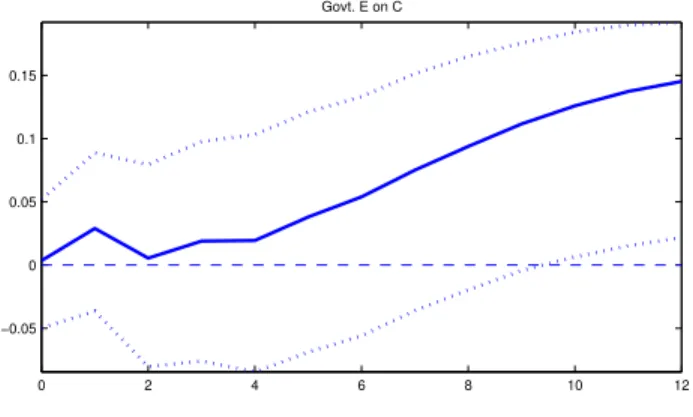
variables. In Figures 3 and 4, we present the responses of private consump-tion to a shock to government spending derived from a standard VAR and our expectation augmented VAR, respectively.27

Both of those responses are basi-cally insignificant. In the model which is not taking into account anticipation, however, consumption turns positive after the ninth quarter. Of course, the insignificant response stands somewhat in contrast to the paper by Blanchard and Perotti (2002). It should be noted, however, that we show the effect on private consumption, not GDP. Moreover, the respective sample periods under consideration are different. Whereas Blanchard and Perotti (2002) base their results on the sample 1960:1 – 1997:4, we not only use data also from the first decade of the new century but in addition include the 1950s. The latter period might be important, which we will discuss below. The main point, though, to be taken from this first set of results, is that at least at this highly aggregated level, taking into account anticipation issues does not overturn the results obtained from a standard VAR.

0 2 4 6 8 10 12 −0.05 0 0.05 0.1 0.15 Govt. E on C

Figure 3: Reaction of private consumption to government expenditure shock. Standard SVAR model without anticipation. Sample: 1947q1-2009q2.

When considering a variable like real government direct expenditure, how-ever, we are lumping together the different subcomponents of this variable, which could have very different effects on private consumption. For example, expenditure on education might have a different effect on economic activity than defense expenditure. Indeed, the crucial feature of models `a la Baxter and King (1993) to generate a negative consumption response to an increase

27_{We plot the point estimate of the impulse response function as well as 68% bootstrap}

confidence bands based on 5000 replications. We show 68% confidence intervals to be com-parable to the literature, e.g., Blanchard and Perotti (2002) or Ramey (2009). Moreover, the corresponding impulse response functions with respect to a shock to government revenue for the current and following specifications can be found in the appendix.

−1 0 2 4 6 8 10 −0.07 −0.06 −0.05 −0.04 −0.03 −0.02 −0.01 0 0.01 Govt. exp. E on C

Figure 4: Reaction of private consumption to anticipated government expen-diture shock. The shock occurs in period 0 and is anticipated in period -1. Sample: 1947q1-2009q2.

in government expenditure is, that the latter represents a withdrawal of re-sources from the economy, which does not substitute or complement private consumption nor contributes to production. Thus, even though government spending might affect utility, it does not influence private decisions except through the budget constraint. However, Baxter and King (1993) show that once government expenditure enters the production function, for example, an increase in this kind of spending can have very expansionary effects depend-ing on the productivity of the good. Consequently, already in the framework of this model, we might expect public expenditure on non-defense items like education, infrastructure, or law enforcement, which probably contribute to aggregate productivity, to induce an increase in private consumption. Public spending on national defense, on the other hand, lacking any complementarity or substitutability with respect to private consumption or any contribution to the private production process, might lead to the opposite response.28

In fact, a change in defense spending is probably the closest approximation to the standard policy experiment conducted in models like Baxter and King (1993), i.e., a setup where in particular unproductive government expenditure are con-sidered. But when we combine those defense and non-defense items in a single variable and study its dynamic effects on private consumption, the respective individual responses might cancel and lead to such weak results as reported

28_{Following the same reasoning, Turnovsky and Fisher (1995) in their theoretical}

investi-gation of the macroeconomic effects of subcomponents of government spending, distinguish “government consumption expenditure” and “government infrastructure expenditure.” The former includes items like national defense or social programs, whereas the latter consists of spending on roads, education, and job training, for example.

above.

Consequently, in order to avoid this blurring of results, we focus in the fol-lowing on different subcomponents of government spending. In particular, we distinguish defense and non-defense expenditure. Considering defense spend-ing is, of course, similar in spirit to Ramey’s (2009) exercise of usspend-ing dummy variables or other more sophisticated measures to capture large increases in government spending related to wars. Thus, we are able to check whether we can replicate Ramey’s (2009) findings in an SVAR-based framework, when taking into account anticipation issues. Our method, however, is not confined to defense spending, so that we can also investigate the role of fiscal foresight when considering non-defense items of government expenditure.29

4.3

Defense expenditure

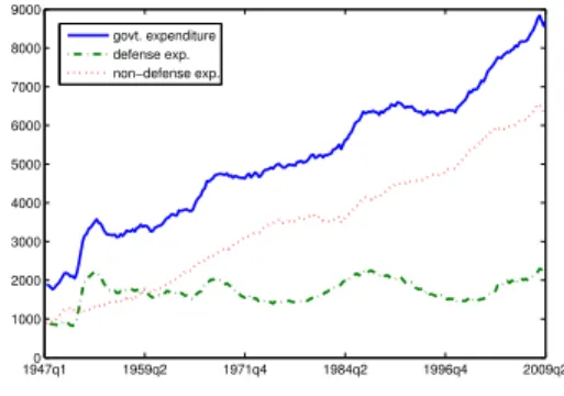
But first, we look at public expenditure on national defense, which exhibits some noticeable features, particularly compared to non-defense spending. Ma-jor movements in total US government expenditure since the 1950s are related to defense spending. Figure 5 shows that while real non-defense expenditure per capita has increased substantially, the increase is rather smooth and fol-lows GDP growth. In contrast, defense spending moved considerably and is rather volatile reflecting the different engagements of the USA in international wars. Most notably, the 1950s are characterized by a strong increase in de-fense expenditure, mainly due to the Korean War build-up. As depicted in Figure 6, this military engagement, along with increased defense spending due to the cold war, led to an increase of the ratio of defense expenditure to GDP from less than 7 percent in 1948 to almost 15 percent in 1952.30

Moreover, the

29_{We distinguish defense and non-defense spending and interpret them in terms of their}

respective degree of substitutability or complementarity or degree of productivity in the private production process in the spirit of Baxter and King (1993) and Turnovsky and Fisher (1995). Another strand of the literature highlights the importance of breaking total government spending down into purchases of goods and services and compensation of public employees (Rotemberg and Woodford 1992, Finn 1998, Forni, Monteforte, and Sessa 2009, Gomes 2009). Our focus, however, is on the different results of the narrative and SVAR approaches concerning the effects of fiscal policy and we therefore highlight defense and non-defense expenditure as subcomponents of total government spending.

30_{Concerning the choice of the sample period, we follow Ramey’s (2008) argument and do}

not disregard the 1950s – including the Korean War – in the subsequent estimations. The Korean War, she forcefully argues, is an important source of variation in the data and should not be ignored. She notes that “[e]liminating the Korean War period from a study of the

correlation between the detrended series of total government spending and de-fense spending is 0.81, whereas it is only 0.39 for total government expenditure and non-defense spending.

1947q10 1959q2 1971q4 1984q2 1996q4 2009q2 1000 2000 3000 4000 5000 6000 7000 8000 9000 govt. expenditure defense exp. non−defense exp.

Figure 5: Real per capita govern-ment spending. 1947q12 1959q2 1971q4 1984q2 1996q4 2009q2 4 6 8 10 12 14 16

Figure 6: Ratio of defense expendi-ture to GDP.

Turning to the estimation results, Figure 7 shows the response of consump-tion to a shock to defense spending derived from a standard fiscal VAR in the spirit of Blanchard and Perotti (2002). Compared to the dynamic response to a shock to total government spending, the point estimate shifts markedly down-wards, in line with our expectations derived from economic theory. However, it is mostly insignificant except for periods 3-5. In particular, the point esti-mate on impact is zero and not significant. A very different picture emerges, when the VAR is augmented with our new methodology to account for antic-ipation effects, depicted in Figure 8. The dynamic response of consumption is unambiguously negative over the entire horizon. In particular, we find that consumption falls on impact with a subsequent slow increase, exactly in line with standard economic models. Even though defense spending does not move before period 0, the private agents respond immediately when they learn about the shock, which occurs in period -1.

Thus, we can reconcile the narrative and SVAR approaches by replicat-ing Ramey’s (2009) findreplicat-ings in an SVAR-based framework. Our results are furthermore in line with Ramey’s (2009) hypothesis, that the difference be-tween those two approaches arises because standard VAR techniques fail to allow for anticipation issues. In order to see those effects clearly, however, it effects of government spending shocks makes as much sense as eliminating the 1990s from a study of the effects of information technology.” Not surprisingly, when disregarding the important period 1947-1959 in the following estimation, we obtain weaker results (Figures A-6 and A-7 in the appendix).

0 2 4 6 8 10 12 −0.1 −0.08 −0.06 −0.04 −0.02 0 0.02 0.04 Govt. def E on C

Figure 7: Reaction of private consumption to government defense expenditure shock. Standard SVAR model without anticipation. Sample: 1947q1-2009q2.

−1 0 2 4 6 8 10 −0.055 −0.05 −0.045 −0.04 −0.035 −0.03 −0.025 −0.02 −0.015 −0.01 −0.005

Govt. exp. def E on C

Figure 8: Reaction of private consumption to anticipated government defense expenditure shock. Sample: 1947q1-2009q2.

is necessary to look at more disaggregated variables to avoid interferences due to potentially different dynamic responses to other items of total government expenditure. All in all, our results underscore the need to appropriately take into account fiscal foresight in empirical research.

We can also look at these results from the viewpoint of the problems related to the misalignment of information sets of private agents and the econometri-cian due to fiscal policy anticipation. In those settings, even though we cannot obtain the true structural shocks from current and past endogenous variables, the system is invertible in current andfuture variables. Thus, as pointed out by Leeper, Walker, and Yang (2009), for example, it is possible to understand the two aforementioned approaches within the single framework of finding instru-ments for future variables. In this regard, it is encouraging that two different approaches of tackling those problems, in particular two different sets of in-struments - “war dummies” on the one hand and future identified shocks to defense spending on the other - yield very similar results.

4.4

Non-defense expenditure

Next, we move to non-defense spending. As explained at the beginning of this section, we might expect private consumption to react differently to rather wasteful defense and potentially productive non-defense expenditure. Since private agents reoptimize and thus respond to new information as soon as it arrives regardless of whether it concerns defense or non-defense items of government spending, fiscal foresight is not confined to changes in the former variable. Thus, we move beyond Ramey’s (2009) exercise and take advantage of the flexibility of our econometric approach, and investigate the consequences of fiscal policy anticipation for dynamic responses to non-defense expenditure. In Figure 9, we plot the impulse-response function of private consumption to a shock to government expenditure, where the latter does not include de-fense spending. It is derived from a three variable VAR estimated over the entire sample period without taking into account anticipation. In this stan-dard framework, we find a significantly positive consumption response after 6 quarters. Thus, the dynamics move broadly in the direction implied by eco-nomic theory. The point estimate, however, is still basically zero on impact and insignificant, and it takes a couple of quarters for the response to move sig-nificantly into positive territory. As Figure 10 makes clear, extending the VAR

0 2 4 6 8 10 12 −0.05 0 0.05 0.1 0.15 0.2 0.25 Govt. nonD E on C

Figure 9: Reaction of private consumption to government non-defense expen-diture shock. Standard SVAR model without anticipation. Sample: 1947q1-2009q2.

to allow for anticipation of fiscal shocks yields a different picture. We now find a significantly positive consumption response already in period -1, when the increase in non-defense expenditure is anticipated. Furthermore, the response stays significantly positive over the entire horizon under consideration, where

after a peak in period 1 it declines steadily. −1 0 2 4 6 8 10 0 0.02 0.04 0.06 0.08 0.1 0.12 0.14 0.16

Govt. exp. nonD E on C

Figure 10: Reaction of private consumption to anticipated government non-defense expenditure shock. Sample: 1947q1-2009q2.

Analogous to the results obtained for defense spending, anticipation effects are also of empirical relevance when considering non-defense expenditure. This finding is in line with Ramey’s (2009) overall argument, even though we ob-tain a significant increase in private consumption. Thus, it is important to distinguish the potentially different dynamic responses to the separate sub-components of total government expenditure.

An unambiguously positive consumption response would be expected when considering the model of Baxter and King (1993) for the case of productive government expenditure, for example.31

Given the opposite findings for defense and non-defense expenditure, the effects of fiscal policy when lumping together those two items in one fiscal aggregate are likely to be weak.

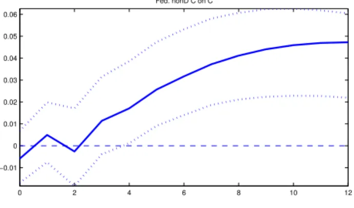
As a final analysis of this section, we take up another point made by Ramey (2009). She argues that aggregate VARs are not very good at capturing shocks to spending which is determined locally. Consequently, in order to make sure that our findings are not driven by the fact that large parts of non-defense expenditure are made by states and local authorities, we look at federal non-defense consumption spending.32

As depicted in Figures 11 and 12, we find our previous results confirmed. In particular, the consumption response derived from our expectation augmented VAR is again significantly positive on impact and over the entire horizon. But also the dynamic response based on a standard

31_{Of course, this result is also in line with the model of Gal´ı, L´opez-Salido, and Vall´es}

(2007), so that this particular set of impulse response functions is not particularly helpful in guiding modeling efforts.

32_{Please note, that since state and local governments do not have expenditure on national}

VAR is very similar. These results suggest that the difference between defense and non-defense spending is not determined by the fact that large parts of non-defense spending are made by states and local authorities.

0 2 4 6 8 10 12 −0.01 0 0.01 0.02 0.03 0.04 0.05 0.06 Fed. nonD C on C

Figure 11: Reaction of private consumption to federal non-defense expenditure shock. Standard SVAR model without anticipation. Sample: 1947q1-2009q2.

−1 0 2 4 6 8 10 0 0.005 0.01 0.015 0.02 0.025

Fed. exp. nonD C on C

Figure 12: Reaction of private consumption to anticipated federal non-defense expenditure shock. Sample: 1947q1-2009q2.

All in all, our findings highlight the importance of taking into account fis-cal foresight when studying empirifis-cally the dynamic effects of changes in fisfis-cal policy on economic activity. Our results are in line with Ramey’s (2009) hy-pothesis, that standard VARs fail to take into account anticipation issues and therefore yield incorrect inferences. Motivated by economic theory, we empha-size the need to look at different subcomponents of total government spending and show with our flexible approach that they have different effects on the macroeconomy. Lumping together the different items in a single fiscal aggre-gate blurs the results. For defense spending, we are able to replicate Ramey’s (2009) findings of a decrease in private consumption in an SVAR-based frame-work and can thereby reconcile the narrative and SVAR approaches of studying

the effects of fiscal policy. For non-defense spending, we also find an impor-tant role for fiscal policy anticipation, but in this case private consumption increases significantly. This result is exactly what would be expected when considering standard neoclassical or New-Keynesian models of fiscal policy for the case of productive public expenditure, for example.

Our findings also correspond to the results of the very recent papers by Kriwoluzky (2009) and Mertens and Ravn (2009). These authors also study the effects of fiscal foresight on the dynamic responses to government expenditure shocks.33

Neither paper, however, looks at subcomponents of total government spending. By distinguishing defense and non-defense spending, we can put their findings into perspective and also qualify the result in an earlier version of this paper of a negative consumption response in an expectation augmented VAR (Tenhofen and Wolff 2007). For instance, similar to our finding for the consumption response to total government expenditure, Kriwoluzky (2009) also obtains a rather weak response in the first couple of quarters. Mertens and Ravn (2009), on the other hand, conclude based on their results that anticipation of fiscal policy does not alter the positive effects of fiscal policy on consumption and output. Finally, from the viewpoint of the problems related to the misalignment of information sets due to fiscal foresight, we find encouraging that different approaches of tackling these problems, in particular different sets of instruments, yield basically the same results. In the next section, we turn to the robustness of our findings.

5

Robustness checks

First, we want to make sure that our results are not driven by the omission of other, potentially important macroeconomic variables. In particular, we consider adding measures of real output and/or a short-term interest rate to the specifications mentioned above.

With respect to the latter variable, while Blanchard and Perotti (2002) also do not control for short-term interest rates, follow-up papers by Perotti add such a variable to a standard fiscal SVAR. Since monetary policy is not

33_{The former employs sign restrictions derived from a DSGE model to identify the}

struc-tural shocks of a vector MA (VMA) model estimated by likelihood methods. The latter consider a vector error-correction model (VECM) and use Blaschke matrices as suggested by Lippi and Reichlin (1993, 1994) to obtain non-fundamental innovations.