Automatic Video Classification: A Survey of the
Literature
Darin Brezeale and Diane J. Cook, Senior Member, IEEE
Abstract—There is much video available today. To help viewers find video of interest, work has begun on methods of automatic video classification. In this paper, we survey the video classifi-cation literature. We find that features are drawn from three modalities–text, audio, and visual–and that a large variety of combinations of features and classification have been explored. We describe the general features chosen and summarize the research in this area. We conclude with ideas for further research.
Index Terms—video classification
I. INTRODUCTION
T
ODAY people have access to a tremendous amount of video, both on television and the Internet. The amount of video that a viewer has to choose from is now so large that it is infeasible for a human to go through it all to find video of interest. One method that viewers use to narrow their choices is to look for video within specific categories or genre. Because of the huge amount of video to categorize, research has begun on automatically classifying video.That automated methods of classifying video are an impor-tant and active area of research is demonstrated by the exis-tence of the TRECVid video retrieval benchmarking evaluation campaign [1]. TRECVid provides data sets and common tasks that allow researchers to compare their methodologies under similar conditions. While much of TRECVid is devoted to video information retrieval, video classification tasks exist as well such as identifying clips containing faces or on-screen text, distinguishing between clips representing outdoor or indoor scenes, or identifying clips with speech or instrumental sound [2].
We focus in this review on approaches to video classifica-tion, and distinguish this from video indexing. The choices of features and approaches taken for video classification are similar to those in the video indexing field. Much of the video indexing research is approached from the database perspective of being able to efficiently and accurately retrieve videos that match a user query [3]. In contrast, video classification algorithms place all videos into categories, typically with a meaningful label associated with each (e.g., ‘sports video’ or ‘comedy video’).
A large number of approaches have been attempted for per-forming automatic classification of video. After reviewing the
Manuscript received March 17, 2007.
D. Brezeale is with the Department of Computer Science and Engineering, The University of Texas at Arlington, Arlington, TX 76019 USA email: ([email protected])
D. Cook is with the School of Electrical Engineering and Computer Science, Washington State University, Pullman, WA 99164-2752 USA (email: [email protected])
literature of methods, we found that these approaches could be divided into four groups: text-based approaches, audio-based approaches, visual-based approaches, and those that used some combination of text, audio, and visual features. Most authors incorporated a variety of features into their approach, in some cases from more than one modality. Therefore, in addition to describing the general features utilized, we also provide summaries of the papers we found published in this area.
The rest of this paper is organized as follows. In section II, we describe some concepts that are generally true regardless of the modality of features used for video classification. In section III, we describe approaches that use text features only. Approaches that use audio features only are described in section IV. In section V, we describe approaches that use visual features only. In section VI, we describe approaches that use combinations of features. We follow the feature descriptions with a comparison of the various features in section VII. We provide conclusions in section VIII and also suggest some ideas for future research in this area.
II. GENERALBACKGROUND
For the purpose of video classification, features are drawn from three modalities: text, audio, and visual. Regardless of which of these are used, there are some common approaches to classification.
While most of the research on video classification has the in-tent of classifying an entire video, some authors have focused on classifying segments of video such as identifying violent [4] or scary [5] scenes in a movie or distinguishing between different news segments within an entire news broadcast [6]. Most of the video classification experiments attempt to classify video into one of several broad categories, such as movie genre, but some authors have chosen to focus their efforts on more narrow tasks, such as identifying specific types of sports video among all video [7]. Entertainment video, such as movies or sports, is the most popular domain for classification, but some classification efforts have focused on informational video (e.g., news or medical education) [8].
Many of the approaches incorporate cinematic principles or concepts from film theory. For example, horror movies tend to have low light levels while comedies are often well-lit. Motion might be a useful feature for identifying action movies, sports, or music videos; low amounts of motion are often present in drama. The way video segments transition from one to the next can affect mood [9]. Cinematic principles apply to audio as well. For example, certain types of music are chosen to produce specific feelings in the viewer [10] [5].
In a review of the video classification literature, we found many of the standard classifiers, such as Bayesian, support
vector machines (SVM), and neural networks. However, two methods for classification are particularly popular: Gaussian mixture models and hidden Markov models. Because of the ubiquitousness of these two approaches, we provide some background on the methods here.
Researchers who wish to use a probabilistic approach for modeling a distribution often choose to use the much stud-ied Gaussian distribution. A Gaussian distribution, however, doesn’t always model data well. One solution to this problem is to use a linear combination of Gaussian distributions, known as a Gaussian mixture model [11]. An unknown probability distribution function p(x) can be represented byK Gaussian distributions such that
p(x) =
K
X
i=1
πiN(x|µi,Σi)
whereN(x|µi,Σi)is theithGaussian distribution with mean µi and covarianceΣi. GMMs have been used for constructing
complex probability distributions as well as clustering. The Hidden Markov model (HMM) is widely used for classifying sequential data. A video is a collection of features in which the order that the features appear is important; many authors chose to use HMMs in order to capture this temporal relationship. An HMM represents a set of states and the probabilities of making a transition from one state to another state [12]. The typical usage in video classification is to train one HMM for each class. When presented with a test sequence of features, the sequence will be assigned to the class whose HMM can reproduce the sequence with the highest probability.
III. TEXT-BASEDAPPROACHES
Text-only approaches are the least common in the video classification literature. Text produced from a video falls into two categories. The first category is viewable text. This could be text on objects that are filmed (scene text), such as an athlete’s name on a jersey or the address on a building, or it could be text placed on-screen (graphic text), such as the score for a sports event or subtitles [7]. Text features are produced from this viewable text by identifying text objects followed by the use of optical character recognition (OCR) [2] to convert these objects to usable text. The text objects can become features themselves, which we discuss in the section on visual features.
The second category is the transcript of the dialog, which is extracted from speech using speech recognition methods [13] or is provided in the form of closed captions or subtitles. Closed captioning is a method of letting hearing-impaired people know what is being said in a video by displaying text of the speech on the screen. Closed captions are found in Line 21 of the vertical blanking interval of a television transmission and require a decoder to be seen on a television [14]. In addition to representing the dialog occurring in the video, closed captioning also displays information about other types of sounds such as sound effects (e.g., [BEAR GROWLS]), onomatopoeias (e.g., grrrr), and music lyrics (enclosed in music note symbols, ). At times, the closed captions may
also include the marks>>to indicate a change of speaker or
>>>to indicate a change of topic [15].
In addition to closed captioning, text can be placed on the television screen with open captioning or subtitling. Open captioning serves the same purpose as closed captioning, but the text is actually part of the video and would need to be extracted using text detection methods and OCR. Subtitles are also part of the video in television broadcasts, although this isn’t necessarily the case for DVDs. However, subtitles are intended for people who can hear the audio of a video but can’t understand it because it is in another language or because the audio is unclear; therefore, subtitles typically won’t include references to non-dialog sounds.
One advantage of text-based approaches is that they can utilize the large body of research conducted on document text classification [16]. Another advantage is that the relationship between the features (i.e., words) and specific genre is easy for humans to understand. For example, few people would be surprised to find the words ‘stadium’, ‘umpire’, and ‘shortstop’ in a transcript from a baseball game.
However, using transcript text does have some disadvan-tages. One is that such text is largely dialog; there is little need to describe what is being seen. For this reason transcript text does not capture much of what is occurring in a video. A second is that not all video has closed captions nor can transcript text be generated for video without dialog. A third is that while extracting closed captions is not computationally expensive, generating the feature vectors of terms and learning from them can be computationally expensive since the feature vectors can have tens of thousands of terms.
Another difficulty in using text-based features is that text derived from speech recognition or OCR of on-screen text has fairly high error rates [17]. While the closed captions for a movie tend to be accurate, closed captions generated in real-time for a news broadcast may suffer from misspellings and omissions.
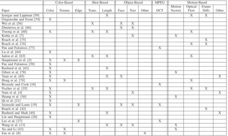
In the next section, we discuss the processing of text features. This is followed by a section describing specific papers that performed video classification using text features only. Papers that utilized text features, whether alone or in combination with other types of features, are listed in Table I.
A. Processing Text Features
A common method for representing text features is to construct a feature vector using the bag-of-words model [22]. In the bag-of-words model, each feature vector has a dimen-sionality equal to the number of unique words present in all sample documents (or closed caption transcripts) with each term in the vector representing one of those words. Each term in a feature vector for a document will have a value equal to the number of times the word represented by that term appears in the document. One potential drawback of the bag-of-words model is that information about word order is not kept.
Representing a transcript may require a feature vector with dimensions in the tens of thousands if every unique word is in-cluded. To reduce the dimensionality, stop lists and stemming are often applied prior to constructing a term feature vector. A
TABLE I
PAPERSUTILIZINGTEXT-BASEDAPPROACHES
Paper Closed Captions Speech Recognition OCR Brezeale and Cook [18] X
Jasinschi and Louie [19] X Lin and Hauptmann [20] X
Qi et al. [21] X
Wang et al. [13] X
Zhu et al. [6] X
stop list is a set of common words such as ‘and’ and ‘the’ [23]. Such words are unlikely to have much distinguishing power and are therefore removed from the master list of words prior to constructing the term feature vectors. Stemming removes the suffixes from words leaving the root. For example, the words ‘independence’ and ‘independent’ both have ‘indepen’ as their root. The stemmed words are used to generate the feature vectors instead of the original words. One of the more common methods for stemming is using Porter’s stemming algorithm [24].
Another common approach is to weight each term using an approach known as the term frequency-inverse document frequency (TF-IDF) approach [25]:
TF-IDF=T F(d, t)×IDF(t)
whereT F(d, t)is the frequency of termt in documentdand
IDF(t)is IDF(t) =log N df(t)
where N is the total number of documents and df(t) is the number of documents containing term t [25].
B. Video Classification Using Text Features Only
Zhu et al. [6] classified news stories using features obtained from closed captions. News video is segmented into stories using the topic change marks inserted by the closed caption annotator. This is followed by applying a natural language parser to identify keywords within a news segment and the first N unique keywords are kept. The authors’ experience is thatN= 20has the best ratio of prediction accuracy to feature length. Classification is performed by calculating weights for each combination of class and keyword. Specifically,
wij =P(ci|fj)2(log(mj) + 1)
is the weight of class i for keywordj whereP(ci|fj)is the
conditional probability of class i given keyword j and mj
is the number of news segments containing keyword j. The weights for all keywords in a news segment are summed and the news segment is assigned to the class with the highest sum. The categories are politics, daily events, sports, weather, entertainment, business and science, health, and technology.
Brezeale and Cook [18] performed classification using text and visual features separately; we describe the use of text features here. Closed captions are extracted from DVDs and represented as term-feature vectors. Classification is performed using a support vector machine, which was chosen because they are well-suited to classification problems in which there
are few training examples but the feature vectors have many terms [26]. There are fifteen genre of movie from the enter-tainment domain.
IV. AUDIO-BASEDAPPROACHES
Audio-only approaches are found slightly more often in the video classification literature than text-only approaches. One advantage of audio approaches is that they typically require fewer computational resources than visual methods. Also, if the features need to be stored, audio features require less space. Another advantage of audio approaches is that the audio clips can be very short; many of the papers we reviewed used clips in the range of 1-2 seconds in length.
To produce features from an audio signal, the signal is sampled at a certain rate (e.g., 22050 Hz). These samples may then be grouped together into frames. Some authors choose to begin one frame where the last ended while others overlap the frames.
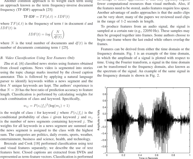
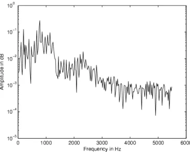
Features can be derived from either the time domain or the frequency domain. Fig. 1 is an example of the time domain, in which the amplitude of a signal is plotted with respect to time. Using the Fourier transform, a signal in the time domain can be transformed to the frequency domain, also known as the spectrum of the signal. An example of the same signal in the frequency domain is shown in Fig. 2.
Fig. 2. Spectrum plot of signal.
A. Audio Features
Whereas many of the visual-based approaches use features intended to represent cinematic principles (to be discussed later), many of the audio-based features are chosen to ap-proximate the human perception of sound. Audio features can lead to three layers of audio understanding [27]: low-level acoustics, such as the average frequency for a frame, mid-level sound objects, such as the audio signature of the sound a ball makes while bouncing, and high-level scene classes, such as background music playing in certain types of video scenes. We provide a brief description of some of the commonly used low-level audio features here.
1) Time-Domain Features: The root mean square (RMS) of the signal energy approximates the human perception of the loudness or volume of a sound [28]. Liu et al. [27] found that sports had a nearly constant level of noise, which can be detected using the volume standard deviation and volume dynamic range. The signal may be subdivided into subbands and the energy of each subband measured separately. Different classes of sounds fall into different subbands [29].
Zero crossing rate (ZCR) is the number of signal amplitude sign changes in the current frame. Higher frequencies result in higher zero crossing rates. Speech normally has a higher variability of the ZCR than in music. If the loudness and ZCR are both below thresholds, then this frame may represent silence.
The silence ratio is the proportion of a frame with amplitude values below some threshold. Speech normally has a higher silence ratio than music. News has a higher silence ratio than commercials.
2) Frequency-Domain Features: The energy distribution is the signal distribution across frequency components. The frequency centroid, which approximates brightness, is the midpoint of the spectral energy distribution and provides a measure of where the frequency components are concentrated [30]. Normally brightness is higher in music than in speech, whose frequency is normally below 7 kHz.
Bandwidth is a measure of the frequency range of a signal
[31]. Some types of sounds have more narrow frequency ranges than others. Speech typically has a lower bandwidth than music.
The fundamental frequency is the lowest frequency in a sample and approximates pitch, which is a subjective measure. The pitch can be undefined for some frames [32]. Pitch is sometimes used to distinguish between male and female speakers. It has also been used to identify significant parts of a person’s speech, such as introduction of a new topic [33]. A frame that is not silent but doesn’t have a pitch may represent noise or unvoice speech [27].
Mel-frequency cepstral coefficients (MFCC) are produced by taking the logarithm of the spectral components and then placing them into bins based upon the Mel frequency scale, which is perception-based. This is followed by applying the discrete cosine transform (DCT) [34]. The DCT has good energy compaction, that is, after transforming a set of values, most of the information needed to reconstruct those values is concentrated in a few of the new values (coefficients). By only keeping those coefficients in which most of the energy is concentrated, the dimensionality can be reduced while still allowing approximations of the original values to be produced.
B. Video Classification Using Audio Features Only
In this section we describe specific papers (listed chronolog-ically) that perform video classification using audio features only. Papers that utilized the most common audio features, whether alone or in combination with other types of features, are listed in Table II.
Liu et al. [27] sample audio signals at 22,050 Hz. These signals are then divided into segments of 1.0 second in length. These segments are subdivided into frames (not to be confused with video frames) of 512 samples each, with a new frame beginning every 128 samples such that each frame overlaps somewhat with the previous three frames. Each clip is represented by a vector with twelve features: non-silence ratio, volume standard deviation, volume dynamic range, frequency component of the volume contour around 4 Hz, pitch standard deviation, voice-or-music ratio, noise-or-unvoice ratio, frequency centroid, frequency bandwidth, energy ratio in the range 0–630 Hz, energy ratio in the range 630–1720 Hz, and energy ratio in the range 1720-4400 Hz. Later analysis found that the features with the most discriminating power are the frequency component of the volume contour around 4 Hz, frequency centroid, frequency bandwidth, energy ratio in the range 0–630 Hz, and energy ratio in the range 1720-4400 Hz. Classification is performed using a one-class-one-network (OCON) structure in which a separate neural network is trained for each class with their output becoming the input to another neural network. The classes of the audio are commercial, basketball game, football game, news report, and weather forecast.
Liu et al. [38] sample an audio signal at 22,050 Hz. This signal is then divided into segments of 1.5 seconds in length. A new segment is begun every 0.5 second so that each segment overlaps with the previous segment by 1.0 second. These segments are subdivided into frames of 512 samples each,
TABLE II
PAPERSUTILIZINGAUDIO-BASEDFEATURES
Time-Domain Frequency Domain
Paper RMS/Energy Subband ZCR Other Freq. Centroid Bandwidth Pitch/Fund. Freq. MFCC
Dinh et al. [29] X X
Fan et al. [8] X X
Fischer et al. [35] X
Huang et al. [36] X X X X X X
Jasinschi and Louie [19] X X X X
Lee et al. [37] X
Liu et al. [27] X X X X X X
Liu et al. [38] X X X X X X
Moncrieff et al. [5] X
Nam et al. [4] X
Pan and Faloutsos [39] X
Qi et al. [21] X
Rasheed and Shah [40] X
Roach and Mason [41] X
Roach et al. [42] X
Wang et al. [13] X X X
Xu and Li [43] X
with a new frame beginning every 256 samples such that each frame overlaps with the previous frame. Each clip is represented by a vector with fourteen features: non-silence ratio, volume standard deviation, standard deviation of zero crossing rate, volume dynamic range, volume undulation, 4 Hz modulation energy, standard deviation of pitch period, smooth pitch ratio, non-pitch ratio, frequency centroid, frequency bandwidth, energy ratio in the range 0–630 Hz, energy ratio in the range 630–1720 Hz, and energy ratio in the range 1720-4400 Hz. An ergodic HMM is trained for each of the five video classes: commercial, basketball game, football game, news report, and weather forecast. Twenty consecutive clips are used as a training sequence for the HMMs.
Roach and Mason [41] use the audio, in particular MFCC, from video for genre classification. This approach is chosen because of its success in automatic speech recognition. The authors investigate how many of the coefficients to keep and find that the best results occur with 10-12 coefficients. A GMM is used because of its popularity in speaker recognition. The genre studied are sports (specifically fast-moving types), cartoons, news, commercials, and music.
Dinh et al. [29] apply a Daubechies 4 wavelet to seven sub-bands of audio clips from TV shows. Like the DCT, wavelet transforms have good energy compaction and are useful for reducing dimensionality. The features for representing the audio clips utilize the wavelet coefficients. They are subband energy, subband variance, and zero crossing rate as well as two features defined by the authors: centroid and bandwidth. Centroid and bandwidth are
centroid= PN i=1i|ωi|2 PN i=1|ωi| 2, and bandwidth= PN i=1(i−centroid) 2|ω i|2 PN i=1|ωi| 2
where N is the number of wavelet coefficients and ωi is
the ith wavelet coefficient. Classification is performed using
the C4.5 decision tree, kNN, and support vector machines
with linear kernels; the best performance results from using the kNN classifier. While clip durations of 0.5, 1.0, 1.5, and 2.0 seconds are tested, they find no significant difference in performance. The genres studied are news, commercials, vocal music shows, concerts, motor racing sports, and cartoons. Wavelets are compared to features from Fourier and time analysis with comparable results.
Pan and Faloutsos [39] investigate the use of independent component analysis (ICA) as applied to visual and audio features separately; we describe the audio-based approach in this section. ICA is a method for finding a set of statistically independent and non-Gaussian components that produced a set of multivariate data [44]. For each class, a set of basis functions are derived. A video is classified as the genre whose basis functions best represent it, with best being defined as the smallest error from reconstructing the clip. To derive the audio basis functions, ICA is applied to a random sample of 0.5 second segments, each of which is down-sampled by a factor of 10. The classes of video are news and commercials. Moncrieff et al. [5] use audio-based cinematic principles to distinguish between horror and non-horror movies. Changes in sound energy intensity are used to detect what the authors call sound energy events [45]. The sound energy events of interest are those associated with the following feelings: surprise or alarm, apprehension, surprise followed by sustained alarm, and apprehension building up to a climax. These four types of sound energy events are found to occur more often in movies classified as horror than those classified as non-horror. Among movies classified as horror, these sound energy events are found to be useful for classifying scenes as well.
V. VISUAL-BASEDAPPROACHES
Most of the approaches to video classification that we surveyed rely on visual elements in some way, either alone or in combination with text or audio features. This corresponds with the fact that humans receive much of their information of the world through their sense of vision.
Of the approaches that utilize visual features, most extract features on a per frame or per shot basis. A video is a
collection of images known as frames. All of the frames within a single camera action are called a shot. A scene is one or more shots that form a semantic unit.1 For example, a conversation between two people may be filmed such that only one person is shown at a time. Each time the camera appears to stop and move to the other person represents a shot change, but the collection of shots that represent the entire conversation is a scene. While some authors use the terms shots and scenes interchangeably, typically when they use the term scene they are really referring to a shot.
Many visual-based approaches use shots since a shot is a natural way to segment a video and each of these segments may represent a higher-level concept to humans, such as “two people talking” or “car driving down road”. Also, a shot can be represented by a single frame, known as the keyframe. Typically the keyframe is the first frame of a shot, although some authors use the term to refer to any single frame that represents a shot. Shots are also associated with some cinematic principles. For example, movies that focus on action tend to have shots of shorter duration than those that focus on character development [46]. One problem with using shot-based methods is that the methods for automatically identifying shot boundaries don’t always perform well [47]. Identifying scenes is even more difficult and there are few video classification approaches that do so.
The use of features that correspond to cinematic principles is popular in the visual-based approaches, more so than in text-based and audio-based approaches. These include using colors as a proxy for light levels, motion to measure action, and average shot length to measure the pace of the video.
One difficulty in using visual-based features is the huge amount of potential data. This problem can be alleviated by using keyframes to represent shots or with dimensionality reduction techniques, such as the application of wavelet trans-forms.
A. Visual Features
1) Color-Based Features: A video frame is composed of a set of dots known as pixels and the color of each pixel is represented by a set of values from a color space [48]. Many color spaces exist for representing the colors in a frame. Two of the most popular are the red-green-blue (RGB) and hue-saturation-value (HSV) color spaces. In theRGBcolor space, the color of each pixel is represented by some combination of the individual colors red, green and blue. In the HSV color space, colors are represented by hue (i.e., the wavelength of the color percept), saturation (i.e., the amount of white light present in the color), and value (also known as the brightness, value is the intensity of the color) [49].
The distribution of colors in a video frame is often rep-resented using a color histogram, that is, a count of how many pixels in the frame exist for each possible color. Color histograms are often used for comparing two frames with the assumption that similar frames will have similar counts even though object motion or camera motion will mean that they don’t match on a per pixel basis. It is impossible to determine
1In rare cases a single shot may contain more than one scene.
from a color histogram the positions of pixels with specific colors, so some authors will divide a frame into regions and apply a color histogram to each region to capture some spatial information.
Another problem with color-based approaches is that the images represented in frames may have been produced under different lighting conditions and therefore comparisons of frames may not be correct. The solution proposed by Drew and Au [50] is to normalize the color channel bands of each frame and then move them into a chromaticity color space. After more processing, including the application of both wavelet and discrete cosine transforms, each frame is now in the same lighting conditions.
2) MPEG: One of the more popular video formats is MPEG (Motion Pictures Expert Group), of which there are several versions. We provide a high-level and somewhat sim-plified description of MPEG-1; for more complete details, consult the MPEG-1 standard [51].
During the encoding of MPEG-1 video, each pixel in each frame is transformed from theRGBcolor space to theY CbCr
color space, which consists of one luminance (Y) and two chrominance (Cb andCr) values. The values in the new color
space are then transformed in blocks of 8×8 pixels using the discrete cosine transform (DCT). Much of the MPEG-1 encoding process deals with macroblocks (MB), which consist of four blocks of8×8 pixels arranged in a2×2 pattern.
Consecutive frames within the same shot are often very similar and this temporal redundancy can be exploited as a means of compressing the video. If a macroblock from a previous frame can be found in the current frame, then encoding the macroblock can be avoided by projecting the position of this macroblock from the previous frame to the current frame by way of a motion vector [52].
Much research has been conducted on extracting features directly from MPEG video, primarily for the purpose of index-ing video [53] [54] [30]. For video classification the primary features extracted from MPEG videos are the DCT coefficients and motion vectors. These can improve the performance of the classification system because the features have already been calculated and can be extracted without decoding the video.
3) Shot-Based Features: In order to make use of shots, they first must be detected. This has proven to be a difficult task to automate, in part because of the various ways of making transitions from one shot to the next. Lienhart [47] states that some video editing systems provide more than 100 different types of edits and no current method can correctly identify all types. Most types of shot transitions fall into one of the following categories: hard cuts, fades, and dissolves. Hard cuts are those in which one shot abruptly stops and another begins [55]. Fades are of two types: a fade-out consists of a shot gradually fading out of existence to a monochrome frame while a fade-in occurs when a shot gradually fades into existence from a monochrome frame. A dissolve consists of one shot fading out while another shot fades in; features from both shots can be seen during this process. While it is important to understand shot transition types in order to correctly identify shot changes, the shot transition types themselves can be useful features for categorization [56].
One of the simplest methods for detecting shots is to take the difference of the color histograms of consecutive frames, with the assumption that the difference in color histograms of frames within the same shot will be smaller than the difference between frames of different shots [57]. This approach, while easy to implement, has a number of potential problems. One is deciding what threshold differences must exceed in order to declare a change in shots. Shots that contain a lot of motion require a higher threshold value than those with little motion. Also, the threshold value is likely to be different for different videos and even within the same video no particular value may correctly identify all shot changes [58]. A threshold value that is too low will identify shot changes that don’t exist while a threshold value that is too high will miss some shot changes. Iyengar and Lippman [59] detect shot changes using the Kullback-Leibler distance between histograms of consecutive frames that have been transformed to thergbcolor space. The
rgb values are calculated using
r= R R+G+B, g= G R+G+B, b= B R+G+B
The Kullback-Leibler distance is calculated using
KL(p||q) =− N X i=1 p(xi)log q(xi) p(xi)
where N is the number of bins in the histograms, p(xi) is
the probability of color xi for one frame and q(xi) is the
probability of color xi for the other frame.
Truong et al. [60] detect shot changes with shot transitions of the types hard cut, fade-in, fade-out, and dissolve [61]. Hard cuts are detected by using a global threshold to identify potential cuts, then a sliding window is applied to these frames using an adaptive threshold. Fade-ins and fade-outs are detected by first identifying monochrome frames and then checking if the first derivative of the luminance mean is relatively constant. Dissolves are identified when the first order difference of the luminance variance curve falls within a range calculated from the luminance variances of the shots preceeding and succeeding the dissolve.
Rasheed and Shah [40] detect shot changes using the inter-section of histograms in the HSV color space. This method works best for hard cuts [62].
Jadon et al. [63] detect shot changes as well as shot tran-sition types using a fuzzy logic based approach [58]. Abrupt changes (i.e., hard cuts) are detected using the intersection of frame histograms in the RGB color space. Gradual changes are detected using pixel differences and intersection of color histograms. The pixel difference between two consecutive frames is calculated using the Euclidean distance between cor-responding pixels in the RGB color space. Gradual changes are further divided into fade-ins and fade-outs, which are detected using pixel differences, intersection of color his-tograms, and edge-pixel counts. After detecting edges using a Sobel edge detector, the difference in the number of pixels of edges between consecutive frames is used to identify fade-in and fade-out transitions. Each feature is fuzzified, that is, values are assigned to qualitative categories (e.g., categorize
as negligible change, small change, or large change). Fuzzy rules are constructed from these features.
Lu et al. [64] avoid detecting shots altogether, instead identifying keyframes using clustering after first transforming frames to a chromatic color space to put all frames under the same lighting conditions.
4) Object-Based Features: Object-based features seem to be uncommon, perhaps because of the difficulty in detecting and identifying objects as well as the computational require-ments to do so. When they are used, they tend to focus on identifying specific types of objects, such as faces [65] [13]. Once objects are detected, features derived from them include dominant color, texture, size, and trajectory.
Dimitrova et al. [66] and Wei et al. [56] use an approach described in [67] for detecting faces. Using images in which the skin-tone pixels have been labeled, a model is learned for the distribution of skin-tones in the Y IQ color space. TheY IQcolor space, a transform of gamma-correctedRGB
values, is used in broadcast video [68]. The skin-tone distribu-tion model is used for identifying regions of skin-tone pixels, which are processed with morphological operations to smooth and combine isolated regions that are related. Finally, shape analysis is applied to identify faces.
Dimitrova et al. [66] and Wei et al. [56] both use an approach described in [69] for identifying text objects within video frames. Using the luminance components of a frame, a process for enhancing the edges is performed followed by edge detection and the filtering of areas unlikely to contain text. Connected component analysis, which identifies pixels that are connected, is performed on the remaining areas to identify text boxes. Text boxes from the same line of text are merged. These text boxes can become objects to be tracked or passed to character recognition software.
Fan et al. [8] detect objects representing a high-level con-cept, such as gastrointestinal regions [70]. The frames from sample clips containing examples of the high-level concept are segmented by identifying regions with homogeneous color or texture. Afterward, a medical consultant annotates those regions matching the high-level concept. Low-level features, such as dominant color and texture, are extracted for these regions and passed to a support vector machine for learning the relationship between features and concept.
5) Motion-Based Features: Motion within a video is pri-marily of two types: movement on the part of the objects being filmed and movement due to camera actions. In some specific types of videos, there might also be other types of movement, such as text scrolling at the bottom of a news program. Motion-based methods largely consist of the use of MPEG motion vectors or the calculation of optical flow.
Optical flow is an estimate of motion in a sequence of images calculated from the velocities of pixel brightness patterns. This could be due to object motion or camera motion. Fig. 3 shows a ball thrown into the air from left to right and the corresponding plot of optical flow values. Measuring optical flow requires multiple video frames; for illustrative purposes, we only show a single frame (the left image in Fig. 3) with a dotted line representing the motion of the ball that the viewer would observe in the preceding and following frames.
Fig. 3. A ball thrown into the air (left) and the optical flow for it (right).
There are many ways to measure optical flow [71]. The method described by Horn and Schunck [72], which is used by several of the papers that we reviewed, determines the optical flow by solving two constraint equations. The gradient constraint equation finds the component of movement in the direction of the brightness gradient. The second constraint is known as the smoothness constraint and is used to determine the component perpendicular to the brightness gradient.
Fischer et al. [35] detect total motion in a shot by comparing the histograms of blocks of consecutive frames. In order to detect object motion, they first calculate optical flow as described in [72]. Motion due to camera movement (e.g., panning) would result in all blocks having motion. Using this, camera motion can be subtracted, leaving only the motion of objects. These objects are identified by segmenting pixels with parallel motion.
Nam et al. [4] measure the motion density within a shot. A 2D wavelet transform is applied to each frame within a shot. A 1D wavelet transform is then applied to the intensity of each pixel in the sequence of 2D-wavelet transformed frames to produce a motion sequence [73]. The dynamic activity of the shot is calculated by
dynamic activity= 1 T e X i=b+1 X m,n |mki(m, n)| !
wherebis the beginning frame,ethe ending frame,T =e−b
is the shot length, andmk
i(m, n)is theithframe of the motion
sequence within thekthshot.
Roach et al. [42] detect the motion of foreground ob-jects using a frame-differencing approach. Pixel-wise frame differencing of consecutive frames is performed using the Euclidean distance between pixels in the RGB color space. These values are thresholded to better represent the motion and doing so for the sequence of pixels produces a 1D signal in the time dimension. To reduce this signal’s sensitivity to camera motions, it is differentiated to produce a final motion signal.
B. Video Classification Using Visual Features Only
In this section we summarize those papers (listed in chrono-logical order) that have utilized visual features only for clas-sifying video. Summary of the main visual-based features and the papers that utilized them, whether alone or in combination with other types of features, can be found in Table III.
Iyengar and Lippman [59] investigated two methods for classification of video. In the first method, they considered
both optical flow and frame differencing as methods for detect-ing motion within video. For each of these, they projected the values to a single dimension. Sequences of these projections became the input to an HMM. They trained one HMM for each of the two input classes: news and sports. They found that the results are similar for both methods, but frame differencing has lower computational requirements.
The second method explores the use of the relationship
A ×C = k from film theory, which states that there is an inverse relationship between the amount of action and character development in a movie. After detecting shots using the Kullback-Leibler distance between histograms in thergb
color space, they calculate the natural log of the ratio of motion energy to shot length. These values become the input to two HMMs, one for action movies and one for character movies. Girgensohn and Foote [74] classify video frames of pre-sentations into six classes: presentation graphics, long shots of the projection screen lit, long shots of the presentation screen unlit, long shots of the audience, medium close-ups of human figures on light backgrounds, and medium close-ups of human figures on dark backgrounds. Frames are extracted from MPEG videos every 0.5 second. Each frame is converted to a 64×64grayscale intensity image. These are then transformed using a discrete cosine transform (DCT) or a Hadamard trans-form (HT). Principal component analysis (PCA) is applied to reduce the dimensionality. PCA takes as input variables
X1, X2, . . . , Xp and finds new values Z1, Z2, . . . , Zp that
are combinations of the input values. These new values are uncorrelated and ordered such thatZ1has the greatest variance andZp the lowest [80]. By keeping only thoseZi terms with
the greatest variance, the original data can be represented in fewer dimensions. The input features to the model are the DCT or HT coefficients with the highest variance as well as the most important principal components. The authors find that the Hadamard transform performed slightly better than the DCT for this application.
Wei et al. [56] classify four types of TV programs: news, commercials, sitcoms, and soap operas. Faces and text are detected and tracked simultaneously to improve performance. The presence of faces or text, the quantity present, and their trajectories are some of the features used for classification. Domain knowledge, specifically how different types of TV programs use distinct or gradual cuts between shots, is found to improve the results. Classification is performed by mapping a video clip into the feature space and finding its weighted distance to the centers of the four classes; the weights are chosen empirically.
Dimitrova et al. [66] extend the work of Wei et al. [56] to classify four types of TV programs: news, commercials, sitcoms, and soap operas. Faces and text are detected and tracked. Counts of the number of faces and text are used for labeling each frame of a video clip. An HMM is trained for each class using the frame labels as the observations.
Truong et al. [60] choose features they believe correspond to how humans identify genre. The features they use are average shot length, percentage of each type of shot transition (cut, fade, dissolve), camera movement, pixel luminance variance, rate of static scenes (i.e., little camera or object motion),
TABLE III
PAPERSUTILIZINGVISUAL-BASEDFEATURES
Color-Based Shot-Based Object-Based MPEG Motion-Based
Motion Optical Frame Paper Color Texture Edge Trans. Length Face Text Other DCT Vectors Flow Diffs Other
Iyengar and Lippman [59] X X X
Girgensohn and Foote [74] X
Wei et al. [56] X X X Dimitrova et al. [66] X X Truong et al. [60] X X X X Kobla et al. [7] X X Roach et al. [75] X Roach et al. [76] X X
Pan and Faloutsos [77] X
Lu et al. [64] X
Jadon et al. [63] X X X
Hauptmann et al. [2] X X X
Pan and Faloutsos [39] X
Rasheed et al. [62] X X
Gibert et al. [78] X X
Yuan et al. [65] X X X X
Hong et al. [79] X X X
Brezeale and Cook [18] X
Fischer et al. [35] X X X X X
Nam et al. [4] X X X
Huang et al. [36] X X
Qi et al. [21] X
Jasinschi and Louie [19] X X X X X
Roach et al. [42] X
Rasheed and Shah [40] X X X
Lin and Hauptmann [20] X
Lee et al. [37] X X
Wang et al. [13] X X X X
Xu and Li [43] X X X
Fan et al. [8] X X X
length of motion runs, standard deviation of a frame luminance histogram, percentage of pixels having brightness above some threshold, and percentage of pixels having saturation above some threshold. Classification is performed using the C4.5 decision tree to classify video into one of five classes: cartoon, commercial, music, news, or sports.
Kobla et al. [7] classify video as either sports or non-sports. Their choice of features are based on cinematic principles and are extracted directly from the compressed domain of MPEG. The features chosen are the use of instant replay, amount of frame text, fraction of frames with motion, the average magnitude and standard deviation of the motion, and the standard deviation of the motion direction. Instant replay is detected using MPEG macroblocks. Classification is performed using a decision tree.
Roach et al. [75] classify video as either cartoon or non-cartoon. The visual feature chosen for classification is the motion of foreground objects, which are detected using pixel-based frame differencing. This produces a second order object motion signal. The dimensionality of this signal is reduced by applying a DCT. The authors investigated how many DCT coefficients to use for constructing the feature vector and found the best results occurred by keeping 4–8 coefficients. Classification is performed using a GMM.
Roach et al. [76] performed classification using only dy-namics, that is, object and camera motion. Camera motion is detected using an optical flow-based approach. Object motion is detected by comparing pixels between consecutive
frames. In both cases the motion is represented by a second order signal. A DCT is applied to these signals to reduce the dimensionality. The first n DCT coefficients from each signal are concatenated to form a feature vector. Classification is performed with a GMM. The video classes were: sport, cartoon, and news.
Pan and Faloutsos [77] use a shot-based method for dis-tinguishing news from commercials. After detecting shots, a graph is constructed from related shots. They found that the graphs for news stories are much larger than the graphs for commercials, which might only consist of a few nodes.
Lu et al. [64] classify a video by first summarizing it. The color channel bands of each frame are normalized and then moved into a chromaticity color space. After more processing including both wavelet and discrete cosine transforms, each frame is now in the same lighting conditions [50]. A set of twelve basis vectors determined from training data can now be used to represent each frame. A hierarchical clustering algorithm segments the video into scenes; the keyframes from the scenes represent the summarized video. One HMM is trained for each video genre with the keyframes as the observation symbols. The video genre are news, commercials, basketball games, and football games.
Jadon et al. [63] chose visual features guided by cinematic principles. Each feature is fuzzified, that is, values are as-signed to qualitative categories (e.g., slow, moderate, fast). Classification rules are learned using a genetic algorithm. The features chosen are editing style (i.e., are shot changes gradual
or abrupt), pace (as measured by shot duration and number of shots), shot activity (measured by the amount of motion in a shot), and camera motion (pan and zoom). Videos are classified as news, sports, or feature films, then news and feature films are sub-classified.
Hauptmann et al. [2] describe the process they used for classifying video shots for the 2002 TREC conference. Video is classified into one of nine classes: outdoors, indoors, cityscape, monologue, face, people, text detection, speech, and instrumental sound. The image features are HSV color histograms of3×3regions of the I-frames from MPEG video, the mean and variance of a texture orientation histogram, an edge direction histogram, and edge direction coherence vector (used to distinguish structured edges). Camera motion and MPEG motion vectors are also investigated but found to be unhelpful. Classification performance is compared for the following classifiers: SVM, kNN, Adaboosting, and decision tree. The SVM performed the best.
Pan and Faloutsos [39] investigate the use of independent component analysis (ICA) as applied to visual and audio features separately; we describe the visual-based approach in this section. For each class, a set of basis functions are derived. A video is classified as the genre whose basis functions best represent it, with best being defined as the smallest error from reconstructing the clip.
To produce the visual features, each frame is divided into 9 regions of n×n pixels each. These pixels and the corre-sponding pixels of the next n−1 frames form a VideoCube. ICA is applied to the red components of the pixels within each VideoCube to derive the video basis functions. The classes of video are news and commercials.
Rasheed et al. [62] used low-level visual features to classify movie previews by genre. Features are chosen with specific cinematic principles in mind. The features are average shot length to measure the tempo of the scene, shot motion content to determine amount of action, lighting key to measure how well light is distributed (i.e., are there shadows) and color variance, which is useful for distinguishing between such genre as comedies (which tend to have bright colors) and horror movies (which tend to be dark).
Clustering is performed using mean-shift clustering. This method is chosen because it can automatically detect the number of clusters and it is non-parametric, so it is unnec-essary to make assumptions about the underlying structure. The genre studied are action, comedy, drama, and horror, but the authors kept in mind that some movies may fall into several genre categories. The mean-shift clustering approach produced six clusters, which are labeled action+drama, drama, comedy+drama, comedy, action+comedy, and horror.
Gibert et al. [78] use motion and color to classify sports video into one of four classes: ice hockey, basketball, football, and soccer. Motion vectors from MPEG video clips are used to assign a motion direction symbol to each video frame. Color symbols are assigned to each pixel of each frame. A symbol for the most prevalent color is assigned to the entire frame. Unlike most other applications of HMMs for video classification, the authors train two HMMs for each video class: one for the frame color symbols and the other for the
motion direction symbols. The output probability for each class is calculated by taking the product of the color and motion output probabilities for that class.
Hong et al. [79] take an object-based approach to clas-sification of video shots. A video is segmented into shots using color histograms and global motion. Up to two objects are identified in each shot, which a human confirms. The objects are represented by color, texture, and trajectory after compensating for any global motion, which results in a 77 term feature vector. In the training phase, a neural network clusters related shots, which is followed by a cluster-to-category mapping to one of twelve categories: five types of vehicle motion and seven types of human motion. In the test phase, the same process is followed for producing the feature vector representing a shot; it is classified by finding the best matching cluster.
Yuan et al. [65] propose two new classification method-ologies using a series of support vector machine classifiers arranged in a hierarchy. The high-level video classes are commercial, news, music video, movie, and sports. The movie class is further divided into action, comedy, horror, and car-toon while the sports class is further divided into baseball, basketball, football, soccer, tennis, and volleyball.
The features are average shot length, cut percentage, av-erage color difference, camera motion (still, pan, zoom, and other), face frames ratio, average brightness, and average color entropy (i.e., color uniformity). A binary tree is constructed using an SVM at each node. In the locally optimal approach, 2-fold cross-validation is used to determine the optimal split of classes at each node into two child nodes. If a child node has two or more classes, it is further split in the same manner. The globally optimal approach also generates a binary tree, but all possible binary trees are considered and cross-validation is used to choose the one with the highest classification accuracy. For example, using the locally optimal approach described above, one possible binary tree may begin with the first level classes: commercial, news, music video, movie, and sports. The best binary split might be commercial in one node and the other four classes in the other node. This second node might be further split into movie in one node and the remaining three classes in the second. When a node contains only the class movie or the class sports, it would then be split in a similar fashion into the various sub-categories of movie and sports.
Brezeale and Cook [18] perform classification using text and visual features separately; we describe the use of visual features here. Video clips in the MPEG-1 format from fif-teen genre of movies are segmented into shots using color histograms in the RGB color space, after which each shot is represented by a keyframe of the DC term of the DCT coefficients. The DC term is proportional to the average value of the block from which it is constructed. By using only the DC terms, each keyframe can be represented using only 1/64 of the total number of DCT coefficients. The keyframes are clustered using ak-means algorithm so that similar shots are grouped together; this allowed each video clip to be represented as a feature vector whose elements are a count of how many of each type of shot are present in the video clip. Classification is performed using a support vector machine.
VI. COMBINATIONAPPROACHES
Many authors chose to use some combination of audio, visual, and text features in an attempt to incorporate the aspects of the viewing process that these features represent and to overcome the weaknesses of each. One difficulty in using features from these three different areas is how to combine the features, which some authors explored. Some chose to combine all features into a single feature vector while others trained classifiers for each modality and then used another classifier for making the final decision.
Fischer et al. [35] use a three-step process to classify video clips by genre. The genre studied are news, car racing (sports), tennis (sports), commercials, and cartoons. In the first step they extract syntactic properties fromRGBframes: color statistics, cuts (or shots), motion vectors, identification of some simple objects, and audio features.
In the second step they derive style attributes using infor-mation found in step 1. This consists of dividing the video into shots using color histograms, using motion information (motion energy is calculated by image subtraction; motion vectors are calculated using an optical flow technique) to distinguish between motion due to the camera panning or zooming and object motion, object segmentation, and dis-tinguishing between the sounds of speech, music, and noise (using frequency and amplitude).
In the third step, modules for each of the style attributes (scene length and transition style, camera motion and object motion, occurrence of recognized objects, audio) estimate the likelihood of the genre represented as a fuzzy set. A weighted average of the estimates is used to produce a final decision.
Nam et al. [4] focus specifically on identifying violent video shots. First, the motion within a shot is measured by applying a 2D wavelet transform to each frame within a shot. A 1D wavelet transform is then applied to the intensity of each pixel in the sequence of 2D-wavelet transformed frames. Those shots whose motion exceeds some predetermined threshold are identified as action shots. Violent action shots are differ-entiated from non-violent action shots by identifying audio and visual signatures associated with gunfire and explosions. Specifically, violence is identified using the colors associated with flames and blood as well as the energy entropy of bursts of sounds produced by gunfire and explosions.
Huang et al. [36] combine audio and visual features for classifying video from the following classes: news reports, weather forecasts, commercials, basketball games, and football games. The audio features produced are as described in [38]. The visual features are dominant color, dominant motion vectors, and the mean and variance of the motion vectors.
Four ways of using these features are investigated. In the first method, the audio and visual features are determined for each clip and concatenated into a single vector. The features vectors for sequences of 20 clips are the input to HMMs, one for each video class. In the second method, audio, color, and motion features are produced for each video frame and a separate HMM is trained for each. The product of the observation probabilities for each these three types of features is used for classification. The third method uses two stages
of HMMs. In the first stage, audio features are used to train HMMs for distinguishing between commercials, football or basketball games, and news reports or weather forecasts. In the second stage, visual features are used to train HMMs to distinguish football games from basketball games and news reports from weather forecasts. For the fourth method, for each of the three types of features (audio, color, motion), an HMM is trained for each class. The output from these HMMs becomes the input to a 3 layer perceptron neural network. The product HMM gave the best average classification accuracy.
Qi et al. [21] classify a stream of news video into types of news stories. Audio and visual features are first used to detect video shots and then these shots are grouped into scenes if necessary. The closed captions and any scene text detected using optical character recognition (OCR) are the features used by a support vector machine for classifying the news stories. Jasinschi and Louie [19] classify TV shows using audio features. Twenty audio features are extracted from 20 ms win-dows that overlap each other by 10 ms. These audio features are used to produce an audio category vector with probability values for six categories: noise, speech, music, speech+noise, speech+speech, and speech+music. Visual features are used to detect commercials. Annotations provided in the closed captions are used to segment the non-commercial parts of a TV program. The audio category vectors for all segments of a show are combined to classify the TV show as either financial news or talk show.
Roach et al. [42] extend their earlier work, classifying video using the audio features described in Roach and Mason [41] as well as visual features obtained in a manner similar to that described in Roach et al. [75]. A GMM is used for classification of a linear combination of the conditional probabilities of the audio and visual features. The video classes are news, cartoons, commercials, sports, music videos.
Rasheed and Shah [40] classify movies by analyzing the previews of the movies using a combination of visual features, audio features, and cinematic principles. The previews are segmented into shots using the intersection of HSV color histograms of the video frames, after which the average shot length is calculated. Using a structural tensor-based approach, the amount of motion in a preview is determined by calculating the visual disturbance (i.e., the ratio of moving pixels to the total pixels in the frame) for each frame in a preview. By plotting the visual disturbance against the average shot length, a linear classifier can separate the action movies from the non-action movies. Action movies are subdivided into those with fire or explosions and those without by analyzing the audio for sudden increases in energy. If the frames corresponding to those points show an increase in pixel intensity, it is assumed that a fire or explosion has occurred. Among non-action movies, light intensity is used to classify movies as comedies, dramas, or horror movies. Comedies tend to have high levels of light intensity while horror movies tend to have low levels. Dramas are somewhere in the middle. Threshold values are used to separate the three genre.
Lin and Hauptmann [20] combine classifiers of visual and text features. A video is divided into shots and a keyframe is extracted from each. Each keyframe is represented by a
vector of the color histogram values in theRGB color space. A support vector machine is trained on these features. For each shot, the closed captions are extracted and represented as a vector. For these vectors, another SVM is trained.
Two methods for combining classifiers are investigated. The first method is based on Bayes’ theorem and uses the product of the posterior probabilities of all classifiers. Performance is improved by assuming equal prior probabilities. The second method uses an SVM as a meta-classifier for combining the results of the other two SVMs. Both methods had similar recall, but the SVM meta-classifier had statistically significant higher precision.
Lee et al. [37] use the DCT coefficients from MPEG video to detect edges for the purpose of classifying scenes of a basketball game. The authors define the term “edgeness” as the total length of edges in a frame. They find that crowded scenes have high edgeness, normal play scenes have medium edgeness, and close-up scenes have low edgeness. Domain knowledge of the duration of an event is used to subcategorize close-up scenes as “goal”, “foul”, or “other” (e.g., the crowd). Many of the foul scenes are misclassified when duration is used alone, so subband energy is measured to detect a referee’s whistle for improving the classification of foul scenes.
Wang et al. [13] classify news video into one of ten categories. Classification is performed primarily using text features. The spoken text from news stories is extracted using speech recognition. Audio features are extracted from one second clips. Forty-nine audio features are produced including 8-order mel-frequency cepstral coefficients, high zero crossing rate ratio, and bandwidth. From each video shot, 14 features are produced including the number of faces, display of closed captions, shot duration, and motion energy.
Using the text features, an SVM produces a confidence vector for each news story. A confidence vector is produced by one GMM per class using the audio features. A confidence vector is also produced by one GMM per class using the visual features. If the confidence vector produced by the SVM using text features exceeds some threshold, then it is used to classify the news story. If not, then an SVM-based meta classifier is used with the input being the concatenation of the text, audio, and visual confidence vectors.
Xu and Li [43] combine audio and visual features for classification. The audio features are the 14 mel-frequency cepstral coefficients. The visual features are the mean and standard deviation of MPEG motion vectors as well as three MPEG-7 visual descriptors: scalable color, color layout, and homogenous texture.
The audio and visual features within a predetermined win-dow (time span) are concatenated into a single feature vector. In addition to synchronizing audio and visual features that are captured at different rates, this allows some temporal information to be represented. Windows of 2 to 40 seconds are tested with the best results occurring using window sizes of 40 seconds. To reduce the dimensionality of the feature vectors, principal component analysis is applied to each. Classification is performed using a GMM. Different numbers of mixture components are tested with the best results occurring with three or more components. The video classes are sports,
cartoon, news, commercial, music.
Fan et al. [8] perform classification using ‘salient’ objects, which the authors define as “the visually distinguishable video components that are related to human semantics.” After identi-fying the salient objects, visual and audio features are extracted for each. The visual features include density ratio, shape, location, color, texture, and trajectory. The audio features include loudness, pitch, and fundamental frequency. A finite mixture model is used to model the relationship between salient objects and the classes. Another contribution of the paper is an adaptive expectation maximization (EM) algorithm for allowing the use of unlabeled samples as well as labeled samples. The authors found that performance improved by including the unlabeled samples. The authors applied their method to the domain of medical education videos using six classes of semantic video concepts.
VII. COMPARISON OFFEATURES
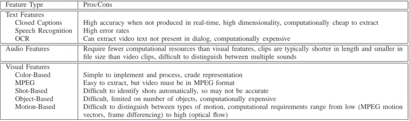
In order to compare different approaches to video classifi-cation, ideally each would be tested on the same data sets and measured using the same metrics, as demonstrated by the TRECVid program. However, from the data descriptions provided in the papers we reviewed, it appears that almost all of the experimental results are based on the use of different data sets. In particular the experiments differed in the number and type of video classes, number of training and testing examples, and length of video clips. The exceptions are the few instances where we reviewed multiple papers from the same authors. In addition, not all of the papers measured the results in the same manner. Most used percent-correctly-classified as the performance metric, but a few measured performance using the recall and precision metrics normally associated with information retrieval. This makes it difficult to compare the approaches reviewed in order to determine which give the best overall results. Therefore, for this reason we focus on describing the advantages and disadvantages of the most common features found in the video classification literature. The pros and cons of the different types of features are summarized in Table IV.
Of the methods for producing text features, extracting closed captions from a television broadcast imposes the fewest computational requirements. It also has the highest accuracy when the closed captions are not produced in real-time, as is the case for some news broadcasts. Dialog transcripts produced using speech recognition have high error rates, especially when sounds besides voices are present; Hauptmann et al. [2] report an error rate of 35–40% when speech and music overlap.
In order to extract text from text objects, potential text regions must be identified first. Some methods for locating text regions in video frames rely on detecting vertical or horizontal edges, which limits their applicability to text that is arranged horizontally [81]. These methods are better suited to extracting the graphic text of a news program than they are for scene text. The performance of OCR is worse when the background is complex [82]. Overall, extracting text from text objects does not perform well in many situations; Hauptmann and Jin [83] report an OCR accuracy of 27%. Some authors have reported
TABLE IV COMPARISON OFFEATURES
Feature Type Pros/Cons Text Features
Closed Captions High accuracy when not produced in real-time, high dimensionality, computationally cheap to extract Speech Recognition High error rates
OCR Can extract video text not present in dialog, computationally expensive
Audio Features Require fewer computational resources than visual features, clips are typically shorter in length and smaller in file size than video clips, difficult to distinguish between multiple sounds
Visual Features
Color-Based Simple to implement and process, crude representation MPEG Easy to extract, but video must be in MPEG format
Shot-Based Difficult to identify shots automatically, so may not be accurate Object-Based Difficult, limited on number of objects, computationally expensive
Motion-Based Difficult to distinguish between types of motion, computational requirements range from low (MPEG motion vectors, frame differencing) to high (optical flow)
much higher accuracy rates when the on-screen text does not vary much in font type and size, as it does in commercials [21].
Representing video using text features typically results in vectors with very high dimensions [20], even after applying stop lists and stemming. Brezeale and Cook [18] report that the term-feature vectors produced from the closed captions of 81 movies had 15,254 terms each. While extracting text features from video may not be time-consuming, processing the text can be due to this high dimensionality.
Text features are especially useful in classifying some genre. Sports [7] and news both tend to have more graphic text than other genre. Text features derived from transcripts are better than audio or visual features at distinguishing between different types of news segments [54].
Audio features require fewer computational resources to obtain and process than visual features [27]. Audio clips are also typically shorter in length and smaller in file size than video clips. Many of the audio-based approaches use low-level features such as ZCR and pitch to segment and describe the audio signal with higher-level concepts such as speech, music, noise, or silence, which are then used for classification. Some of these approaches assume that the audio signal will only represent one of these high-level concepts [84], which is unrealistic for many real-life situations.
Most of the visual-based features rely in some manner on detecting shot changes and are therefore dependent on doing so correctly. This is the case whether the feature is the shot itself, such as average shot length, or applied at the shot level, such as average motion within a shot. Detecting shot changes automatically is still a difficult problem, primarily due to the variety of forms transitions between shots can take [47].
Frame-based features are costly to produce if each frame is to be considered. This also results in a tremendous amount of data to process for full-length movies. This can be made easier by only processing some frames, such as the keyframes of video shots. This assumes that the keyframe chosen is representative of the entire shot. This assumption will be violated if there is much motion in the shot.
Color-based features are simple to implement and inexpen-sive to process. They are useful in approaches wishing to use cinematic principles. For example, amount and distribution of light and color set mood [62]. Some disadvantages are that
color histograms lose spatial information and color-based com-parisons suffer when images are under different illumination conditions [64]. The crudeness of the color histogram also means that frames with similar color distributions will appear similar regardless of the actual content. For example, the color histogram of a video frame containing a red apple on a blue tablecloth may appear similar to the histogram of a red balloon in the sky.
Object-based features can be costly and difficult to derive. Wei et al. [56] report that detecting text objects is efficient enough to be applied to all video frames but that detecting faces is so expensive that they limited it to the first few frames of each shot. Most methods require that the objects be somewhat homogenous in color or texture in order to segment them correctly, which may also require confirmation from humans [79]. Objects that changed shape, such as clouds, would also prove difficult to handle.
The quantity of motion in a video is useful in a broad sense, but it is not sufficient by itself in distinguishing between the types of video that typically have large quantities of motion, such as action movies, sports, and music videos [4]. Calculat-ing the quantity of motion in a shot includes usCalculat-ing optical flow, MPEG motion vectors, or frame differencing. Optical flow is costly to calculate and may not match the direction of the real motion, if that is also required. For example, if the camera panned to the left then the optical flow would indicate that the motion moves to the right. The optical flow algorithm of Horn and Schunck has problems with occluded edges since they cause a discontinuity in reflectance [72]. Extracting motion vectors from MPEG-encoded video is not costly, but of course requires that the video be in this video format in the first place. However, motion as indicated by motion vectors may be less accurate than motion as measured using optical flow [54]. Iyengar and Lippman [59] found that measuring motion using frame differencing produced results similar to those that measured motion using optical flow, yet frame differencing is simpler to implement and less computationally expensive. However, region-based features such as frame differencing are non-specific as to the direction of the motion [75].
Measuring specific types of motion, such as object motion or camera motion, is also a difficult problem because of the difficulty in separating the two. Many approaches for measur-ing the motion of objects require that the object be segmented,