Object Recognition in 3D Point Clouds Using
Web Data and Domain Adaptation
Kevin Lai
Dieter Fox
Department of Computer Science & Engineering
University of Washington, Seattle, WA
Abstract
Over the last years, object detection has become a more and more active field of research in robotics. An important problem in object detection is the need for sufficient labeled training data to learn good classifiers. In this paper we show how to significantly reduce the need for manually labeled training data by leveraging data sets available on the World Wide Web. Specifically, we show how to use ob-jects from Google’s 3D Warehouse to train an object detection system for 3D point clouds collected by robots navigating through both urban and indoor environments. In order to deal with the different characteristics of the web data and the real robot data, we additionally use a small set of labeled point clouds and performdomain adaptation. Our experiments demonstrate that additional data taken from the 3D Warehouse along with our domain adaptation greatly improves the classification accuracy on real-world environments.
1
Introduction
In order to operate safely and efficiently in populated urban and indoor environments, autonomous robots must be able to distinguish between objects such as cars, people, buildings, trees, chairs and furniture. The ability to identify and reason about objects in their environment is extremely useful for autonomous cars driving on urban streets as well as robots navigating through pedestrian areas or operating in indoor environments. Domestic housekeeping and elderly care robots will need the ability to detect, classify and locate common objects found in indoor environments if they are to perform useful tasks for people. A key problem in this context is the availability of sufficient labeled training data to learn classifiers. Typically, this is done by manually labeling data collected by the robot, eventually followed by a procedure to increase the diversity of that data set (Sapp et al., 2008). However, data labeling is error prone and extremely tedious. We thus conjecture that relying solely on manually labeled data does not scale to the complex environments robots will be deployed in.
The goal of this research is to develop techniques that significantly reduce the need for labeled training data for classification tasks in robotics by leveraging data available on the World Wide Web. Unfortunately, this is not as straightforward as it seems. A key problem is the fact that the data available on the World Wide Web is often very
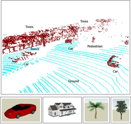
Figure 1: (Upper row) Part of a 3D laser scan taken in an urban environment (ground plane points shown in cyan). The scan contains multiple cars, a person, a fence, and trees in the background. (lower row) Example models from Google’s 3D Warehouse.
different from that collected by a mobile robot. For instance, a robot navigating through an urban environment will often observe cars and people from very close range and at angles different from those typically available in data sets such as LabelMe (Russell et al., 2008). Furthermore, weather and lighting conditions might differ significantly from web-based images.
The difference between web-based data and real data collected by a robot is even more obvious in the context of classifying 3D point cloud data. A number of online shape databases have emerged in recent years, including the Princeton Shape Bench-mark (Shilane et al., 2004) and Google’s 3D Warehouse (Google, 2008). Google’s 3D Warehouse is particularly promising, as it is a publicly available database where any-one can contribute models created using Google’s SketchUp 3D modeling program. It already contains tens of thousands of user-contributed models such as cars, street signs, furniture, and common household objects. In this paper, we use objects from Google’s 3D Warehouse to help classify 3D point clouds collected by mobile robots in both urban terrain (see Fig. 1) and an indoor tabletop scenario (see Fig. 2). We would like to leverage such an extremely rich source of freely available and labeled training data. However, virtually all objects in this dataset are created manually and thus do not accurately reflect the data observed by actual range sensing devices.
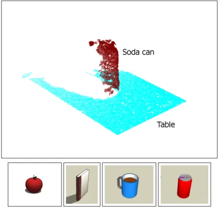
Figure 2: (Upper row) Part of a point cloud taken in an indoor environment (table plane points shown in cyan). The scan contains a single soda can. (lower row) Example models from Google’s 3D Warehouse.
The aim of domain adaptation is to use large sets of labeled data from one domain along with a smaller set of labeled data from the target domain to learn a classifier that works well on the target domain. In this paper we show how domain adaptation can be applied to the problem of object detection in 3D point clouds. The key idea of our ap-proach is to learn a classifier based on objects from Google’s 3D Warehouse along with a small set of labeled point clouds. Our classification technique builds on an exemplar-based approach developed for visual object recognition (Malisiewicz and Efros, 2008). To obtain a final labeling of individual 3D points, our system first labels a soup of seg-ments (Malisiewicz and Efros, 2007) extracted from the point cloud. Each segment is classified based on the labels of exemplars that are “close” to it. Closeness is measured via a learned distance function for spin image signatures (Johnson and Hebert, 1999; Assfalg et al., 2007) and other shape features. We show how the learning technique can be extended to enable domain adaptation. In the experiments we demonstrate that additional data taken from the 3D Warehouse along with our domain adaptation greatly improves the classification accuracy on point clouds of real-world environments.
This paper makes the following key contributions:
un-derstanding in 3D point clouds. To do so, we enhance a technique developed for visual object recognition with 3D shape features and introduce a probabilistic, exemplar-based classification method. Our resulting approach significantly out-performs alternative techniques such as boosting and support vector machines.
• We demonstrate how to leverage large, human-generated datasets such as Google’s 3D Warehouse to further increase the performance of shape-based object recog-nition. To do so, we introduce two techniques fordomain adaptation, one based on previous work done in the context of natural language processing and one we developed specifically for our exemplar-based approach.
This paper is organized as follows. In the next section, we provide background on exemplar-based learning and on the point cloud segmentation method used in our sys-tem. Then, in Section 3, we show how the exemplar-based technique can be extended to the domain adaptation setting. Section 4 introduces a method for probabilistic clas-sification. Experimental results are presented in Section 5, followed by a discussion of related work and conclusions.
2
Learning Exemplar-based Distance Functions for 3D
Point Clouds
In this section we describe the details of our approach to point cloud classification. We review the exemplar-based recognition technique introduced in Malisiewicz and Efros (2008). While the approach was developed for vision-based recognition tasks, we show how to adapt the method to object recognition in point clouds. In a nutshell, the approach takes a set of labeled segments and learns a distance function for each segment, where the distance function is a linear combination of feature differences. The weights of this function are learned such that the decision boundary maximizes the margin between the associated subset of segments belonging to the same class and segments belonging to other classes.
2.1
Point Cloud Segmentation and Feature Extraction
Given a 3D point cloud of a scene, we first segment out points belonging to the ground from points belonging to potential objects of interest. In our indoor dataset, we assume that the objects are located on a table, which allows us to extract the ground plane via straightforward RANSAC plane fitting. For the more complex outdoor scenes, we first bin the points into grid cells of size25×25×25cm3, and run RANSAC plane
fitting (Fischler and Bolles, 1981) on each cell to find the surface orientations of each grid cell. We take only the points belonging to grid cells whose orientations are less than30 degrees with the horizontal and run RANSAC plane fitting again on all of these points to obtain the final ground plane estimation. The assumption here is that the ground has a slope of less than30degrees, which is usually the case and certainly for our data sets. Points close to the extracted plane are labeled as “ground” and not considered in the remainder of our approach. Fig. 1 displays a Velodyne LIDAR scan
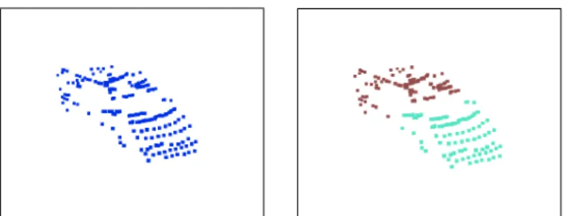
Figure 3: (left) Point cloud of a car extracted from a laser scan. (right) Segmentation via mean-shift. The soup of segments additionally contains a merged version of these segments.
of a street scene with the extracted ground plane points shown in cyan, while Fig. 2 shows a point cloud of an indoor scene.
Since the extent of each object is unknown, we perform segmentation to obtain indi-vidual object hypotheses. We experimented with the mean-shift clustering (Comaniciu and Meer, 2002) and normalized cuts (Shi and Malik, 2000) algorithms at various pa-rameter settings and found that the former provided better segmentation. In the context of vision-based recognition, (Malisiewicz and Efros, 2007) showed that it is beneficial to generate multiple possible segmentations of a scene, rather than relying on a single, possibly faulty segmentation. Similar to their technique, we generate a “soup of seg-ments” using mean-shift clustering and considering merges between clusters of up to3
neighboring segments. An example segmentation of a car automatically extracted from a complete scan is shown in Fig. 3. The soup also contains a segment resulting from merging the two segments.
We next extract a set of features capturing the shape of a segment. For each point, we compute spin image features (Johnson and Hebert, 1999), which are16×16 ma-trices describing the local shape around that point. Following the technique introduced by Assfalg et al. (2007) in the context of object retrieval, we compute for each point a spin image signature, which compresses information from its spin image down to an 18-dimensional vector. Representing a segment using the spin image signatures of all its points would be impractical, so the final representation of a segment is composed of a smaller set of spin image signatures. In Assfalg et al. (2007), this final set of sig-natures is obtained by clustering all spin image sigsig-natures describing an object. The resulting representation is rotation-invariant, which is beneficial for object retrieval. However, in our case the objects of concern usually appear in a constrained range of orientations. Cars and trees are unlikely to appear upside down, for example. The orientation of a segment is actually an important distinguishing feature and so unlike in Assfalg et al. (2007), we partition the points into a3×3×3grid and performk -means clustering on the spin image signatures within each grid cell, with a fixedk= 3. Thus, we obtain for each segment3·3·3 = 27shape descriptors of length3·18 = 54
each. We also include as features the width, depth and height of the segment’s bound-ing box, as well as the segment’s minimum height above the ground. This gives us a total of27 + 4 = 31descriptors.
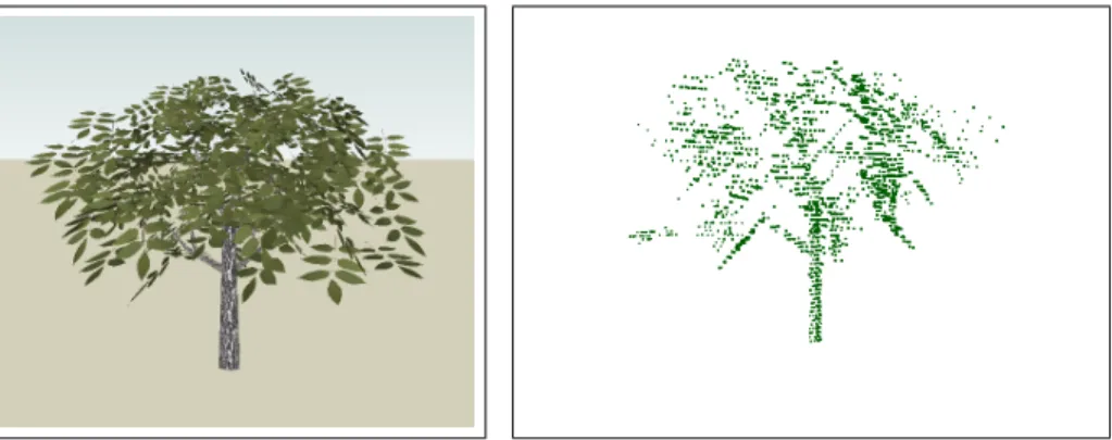
Figure 4: (left) Tree model from the 3D Warehouse and (right) point cloud extracted via ray casting.
To obtain similar representations of models in the 3D Warehouse, we perform ray casting on the models to generate point clouds and then perform the same procedure described in the previous paragraph (see Fig. 4).
2.2
Learning the Distance Function
Assume we have a set ofnlabeled point cloud segments,E ={e1, e2, . . . , en}. We
refer to these segments asexemplars,e, since they serve as examples for the appearance of segments belonging to a certain class. Let fe denote the features describing an
exemplare, and letfzdenote the features of an arbitrary segmentz, which could also
be an exemplar. dez is the vector containing component-wise,L2distances between
individual features describingeandz:dez[i] =||fe[i]−fz[i]||. In our case, featuresfe
andfzare the31descriptors describing segmenteand segmentz, respectively.dezis a
31+1dimensional distance vector where each component,i, is theL2distance between
featureiof segmentseandz, with an additional bias term as described in Malisiewicz and Efros (2008). Distance functions between two segments are linear functions of their distance vector. Each exemplar has its own distance function,De, specified by
the weight vectorwe:
De(z) =weTdez (1)
Note that since each exemplar has its own set of weights, the functions do not define a true distance metric, as it is asymmetric. Instead, a given exemplar e’s function evaluates the similarity of other exemplars toebased on a particular weighing of feature differences learned specifically fore. This is advantageous since different exemplars may have different sets of features that are better for distinguishing itself from other exemplars.
To learn the weights of this distance function, it is useful to define a binary vector
αe, the length of which is given by the number of exemplars with the same label ase.
During learning,αeis non-zero for those exemplars that are ine’s class and that should
be similar toe, and zero for those that are in the same class but considered irrelevant for exemplare. The key idea behind these vectors is that even within a class, different
segments can have very different feature appearance. This could depend, for example, on the angle from which an object is observed.
The values ofαeandweare determined for each exemplar separately by the
fol-lowing optimization: {w∗e,α∗e}= argmin we,αe X i∈Ce αeiL(−wT edei) + X i6∈Ce L(wTedei) subject towe≥0; αei∈ {0,1}; X i αei=K (2)
Here, Ce is the set of examplars that belong to the same class as e,αei is thei-th
component ofαe, andLis the squared hinge loss function. The constraints ensure thatK values ofαe are non-zero. In (2), theK positive exemplars are considered via the non-zero terms in the first summation, and the negative exemplars are given in the second summation. The resulting optimization aims at maximizing the margin of a decision boundary that hasK segments frome’s class on one side, while keeping exemplars from other classes on the other side. The optimization procedure alternates between two steps. Theαevector in thek-th iteration is chosen such that it minimizes
the first sum in (2):
αke = argmin αe X i∈Ce αeiL(−wkT e dei) (3)
This is done by simply settingαk
eto 1 for theKsmallest values ofL(−wTedei), and
setting it to zero otherwise. The next step fixesαetoαk
eand optimizes (2) to yield the
newwek+1: wke+1= argmin we X i:∈Ce αkeiL(−w T edei) + X i6∈Ce L(wTedei) (4)
When choosing the loss functionLto be the squared hinge loss function, this optimiza-tion yields standard Support Vector Machine learning (Boser et al., 1992). The iterative procedure converges whenαke=αke+1. Malisiewicz and Efros (2008) showed that the
learned distance functions provide excellent recognition results for image segments.
3
Domain Adaptation
So far, the approach assumes that the exemplars in the training setEare drawn from the same distribution as the segments on which the approach will be applied. While this worked well in Malisiewicz and Efros (2008), it does not perform well when training and test domain are significantly different. In our scenario, for example, the classifica-tion is applied to segments extracted from 3D point clouds, while most of the training data is extracted from the 3D Warehouse data set. As we will show in the experimental results, combining training data from both domains can improve classification over just using data from either domain, but this performance gain cannot be achieved by simply combining data from the two domains into a single training set.
In general, we distinguish between two domains. The first one, thetarget domain, is the domain on which the classifier will be applied after training. The second domain, thesource domain, differs from the target domain but provides additional data that can help to learn a good classifier for the target domain. In our context, the training data now consists of exemplars chosen from these two domains:E =Et ∪ Es. Here,Et
contains exemplars from the target domain, that is, labeled segments extracted from the real laser data.Escontains segments extracted from the 3D Warehouse. As typical
in domain adaptation, we assume that we have substantially more labeled data from the source domain than from the target domain: |Es| |Et|. We now describe two
methods for domain adaptation in the context of the exemplar-based learning technique.
3.1
Domain Adaptation via Feature Augmentation
Daum´e III (2007) introduced feature augmentation as a general approach to domain adaptation. It is extremely easy to implement and has been shown to outperform var-ious other domain adaptation techniques and to perform as well as the thus far most successful approach to domain adaptation (Daum´e III and Marcu, 2006). The approach performs adaptation by generating a stacked feature vector from the original features used by the underlying learning technique. Specifically, letfe be the feature vector
describing exemplare. The approach in Daum´e III (2007) generates a stacked vector
f∗ e as follows: fe∗= fe fs e ft e (5) Here,fs
e =feifebelongs to the source domain, andfes =0if it belongs to the target
domain. Similarly,ft
e =feifebelongs to the target domain, andfet =0otherwise.
Using the stacked feature vector, it becomes clear that exemplars from the same domain are automatically closer to each other in feature space than exemplars from different domains. Daum´e III (2007) argued that this approach works well since data points from the target domain have more influence than source domain points when making predictions about test data.
3.2
Domain Adaptation for Exemplar-based Learning
We now present a method for domain adaptation specifically designed for the exemplar-based learning approach. The key difference between our domain adaptation technique and the single domain approach described in Section 2 lies in the specification of the binary vectorαe. Instead of treating all exemplars in the class ofethe same way, we distinguish between exemplars in the source and the target domain. Specifically, we use the binary vectorsαs
eandαtefor the exemplars in these two domains. The domain
adaptation objective becomes
{w∗ e,α s∗ e ,α t∗ e}= argmin we,αs e,αte X i∈Cs e αseiL(−wTedei) + X i∈Ct e αteiL(−wTedei) + X i6∈Ce L(wTedei), (6)
whereCs eandC
t
eare the source and target domain exemplars with the same label ase.
The constraints are virtually identical to those for the single domain objective (2), with the constraints on the vectors becomingP
iα s ei=K sandP iα t ei=K t. The values
forKsandKtgive the number of source and target exemplars that must be considered during the optimization.
The subtle difference between (6) and (2) has a substantial effect on the learned distance function. To see this, imagine the case where we train the distance function of an exemplar from the source domain. Naturally, this exemplar will be closer to source domain exemplars from the same class than to target domain exemplars from that class. In the extreme case, the vectors determined via (3) will contain 1s only for source domain exemplars, while they are zero for all target domain exemplars. The single domain training algorithm will thus not take target domain exemplars into account and learn distance functions for source domain exemplars that are good in classifying source domain data. There is no incentive to make them classify target domain exemplars well. By keeping two differentα-vectors, we can force the algorithm to optimize for classification on the target domain as well. The values forKsandKt
allow us to trade off the impact of target and source domain data. They are determined via grid search using cross-validation, where the values that maximize the area under the precision-recall curve are chosen.
The learning algorithm is very similar to the single domain algorithm. In thek -th iteration, optimization of -theα-vectors is done by settingαs k
e andαt ke to 1 for the
exemplars yielding theKsandKtsmallest loss values, respectively. Then, the weights
wk+1
e are determined via convex SVM optimization (Keerthi et al., 2006) using the
most recentα-vectors within (6).
4
Probabilistic Classification
To determine the class of a new segment,z, we first determine the set of associated ex-emplars, which are those for whichDe(z)≤1. This corresponds to all exemplarsefor
whichzfall one’s side of the decision boundary. Malisiewicz and Efros (2008) showed that this threshold is not only natural, but also empirically gave good performance. We found this to be the case as well.
In Malisiewicz and Efros (2008), segment z is labeled with the majority class among the associated exemplars. However, this approach does not model the reliability of individual exemplars and does not lend itself naturally to a probabilistic interpreta-tion. Furthermore, it does not take into account that the target domain is different from the source domain.
To overcome these limitations, we choose the following Na¨ıve Bayes model over exemplars. We define the class-conditional probability for each exemplarein the train-ing set to be p(e|c) := | {e 0|D e(e0)≤1} | Nc , (7)
wheree0are target domain training exemplars in classcandNcis the number of target
the proportion of exemplarse0in classcthat are close toe(De(e0)≤1). We use only
target domain exemplars because the ultimate goal is to label segments from the target domain only.
Given a set of exemplarsE, the class-conditional probability of a test segmentzis defined to be p(z|c) := Y e∈E ∧De(z)≤1 p(e|c)/ X c0 Y e∈E ∧De(z)≤1 p(e|c0). (8)
Here we have assumed independence between the class-conditional probability dis-tributions over exemplars. Intuitively, the class-conditional distribution ofzshould be similar to that of exemplars that are similar to it and (8) captures this. The denominator is a normalization factor to ensure that we have indeed defined a probability distribu-tion. Applying Bayes’ rule, the probability that segmentzbelongs to classcis simply
p(c|z) =Pp(c)p(z|c)
c0p(c0)p(z|c0)
. (9)
The priorp(c)is estimated via class frequencies in the target domain training data. We can apply the results of the above segment classification to individual points. As described in Section 2.1, we extract a soup of segments from a 3D point cloud. Thus, each point may belong to multiple segments. Using the probability distributions over the classes of these segments, the distribution over the class of a single pointlis given by
p(c|l) ∝ Y
z∈Zl
p(c|z), (10)
whereZlis the set of segments that contain pointl. This combines the class hypotheses
from multiple segments in the “soup” in a probabilistic manner to produce the final classification. In our setup, points in a test scene are assigned to the class with the highest probability.
5
Experiments
We evaluate the different approaches to 3D point cloud classification mostly in the context of outdoor scenes. The task here is to segment and classify point clouds col-lected in an urban environment into the following seven classes: cars, people, trees, street signs, fences, buildings, and background. Our experiments demonstrate that our two domain adaptation methods lead to improvements over approaches without domain adaptation and alternatives including LogitBoost (Friedman et al., 2000) and a regular Multi-class SVM (Chang and Lin, 2001). In particular, our exemplar-based domain adaptation approach obtains the best performance. To demonstrate that our approach can be applied to different environments and sensors, we also show results on detecting tabletop objects belonging to six classes: apple, book, laptop, mug, soda can, and water bottle.
Our exemplar-based learning code is based on a MATLAB implementation pro-vided by Malisiewicz. The distance function learning takes around 15 minutes. We
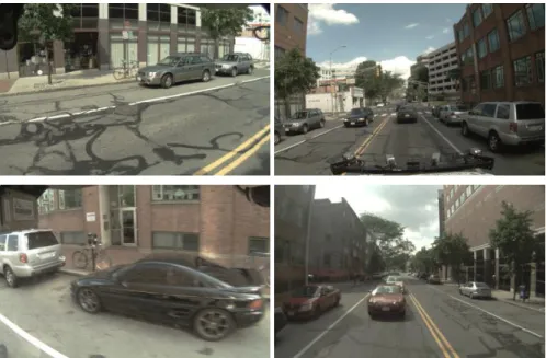
Figure 5: A scene from the urban driving data set. Starting with the image in the top left and going clockwise, they are captured with left-, forward-, right-, and rear-facing cameras mounted on the vehicle.
implemented the classification phase as a single-threaded C++ application. It takes on average 80 seconds to classify an outdoor scene and 17 seconds to classify an indoor scene. For outdoor scenes, which are large and complex, the majority of the time (60 seconds) is consumed by segmentation and feature extraction. For indoor scenes, these two steps take a negligible amount of time. In both cases, computing the distances be-tween every test segment to every training exemplar currently takes 10 seconds. Much of the procedure, including the distance computation, operates on the different test seg-ments and training exemplars independently; the code is highly parallelizable. Hence, a multi-threaded CPU or GPU implementation should speed this up to near real-time performance.
5.1
Urban Driving Data Set
We evaluated our approach using models from the Google 3D Warehouse as our source domain set,Es, and ten labeled street scenes as our target domain set, Et. The ten
scenes, collected by a Velodyne LIDAR mounted on a vehicle navigating through the Boston area, were chosen so that they did not overlap spatially. Each scene is a single rotation of the LIDAR, yielding a cloud of nearly 70,000 points. Scenes may contain objects including, but not limited to, cars, bicycles, buildings, pedestrians and street signs. Camera images taken at one of these scenes are shown in Fig. 5. Manual label-ing of 3D scans was done by inspectlabel-ing the camera data collected along with the laser data. We automatically downloaded the first 100 models of each of cars, people, trees,
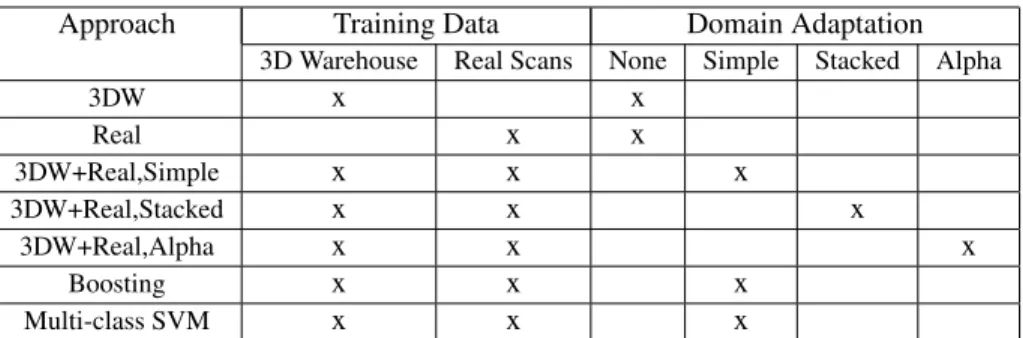
Approach Training Data Domain Adaptation
3D Warehouse Real Scans None Simple Stacked Alpha
3DW x x Real x x 3DW+Real,Simple x x x 3DW+Real,Stacked x x x 3DW+Real,Alpha x x x Boosting x x x Multi-class SVM x x x
Table 1: Table summarizing the training data and domain adaptation methods used in the approaches compared in Section 5.2.
street signs, fences and buildings from the Google 3D Warehouse and manually pruned out low quality models, leaving around 50 models for each class. We also included a number of models to serve as the background class, consisting of various other objects that commonly appear in street scenes, such as garbage cans, traffic barrels and fire hydrants. Recall that orientation information is preserved in our feature representation. To account for natural orientations that the objects can take in the environment, we generated 10 simulated laser scans from evenly-spaced viewpoints around each of the downloaded models, giving us a total of around 3,200 exemplars in the source domain set. The ten labeled scans totaled to around 400 exemplars in the six actual object classes. We generate a “soup of segments” from these exemplars, using the data points in real scans not belonging to the six actual classes as candidates for additional back-ground class exemplars. After this process, we obtain a total of 4,900 source domain segments and 2,400 target domain segments.
5.2
Comparison with Alternative Approaches
We compare the classification performance of our exemplar-based domain adaptation approach to several approaches, including training the single domain exemplar-based technique only on Warehouse exemplars, training it only on the real scans, and training it on a mix of Warehouse objects and labeled scans. The last combination can be viewed as a na¨ıve form of domain adaptation. We also tested the stacked feature approach to domain adaptation described in Section 3.1. The different approaches being compared are summarized in Table 1. “3DW” stands for exemplars from the 3D Warehouse, and “Real” stands for exemplars extracted from the Velodyne laser scans. Where exemplars from both the 3D Warehouse and real scans are used, we also specify the domain adaptation technique used. By “Simple” we denote the na¨ıve adaptation of only mixing real and Warehouse data. “Stacked” refers to the stacked feature approach, applied to the single domain exemplar technique. Finally, “Alpha” is our exemplar-based domain adaptation technique.
The optimal K values (number of non-zero elements in theα vectors) for each approach were determined separately using grid search and cross validation. Where training involves using real scans, we repeated each experiment10times using random
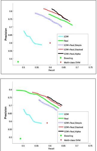
Figure 6: Precision-recall curves comparing performance of the various approaches trained using five (upper panel) and three (lower panel) real scans where applicable.
train/test splits of the10total available scans. Each labeled scan contains around 240 segments on average.
The results are summarized in Fig. 6. Here the probabilistic classification described in Section 4 was used and the precision-recall curves were generated by varying the probabilistic classification threshold between[0.5,1]. The precision and recall values are calculated on a per-point basis over entire scenes, including all seven object classes, but omitting the ground plane points. Note that this evaluation criterion is different from the evaluation used in Malisiewicz and Efros (2008), where they considered any correctly labeled segment with an overlap of more than50%with a ground truth object to be correct. Each curve in Fig. 6 corresponds to a different experimental setup. The left plot shows the approaches trained on five real scans, while the right plot shows the approaches trained on three real scans. All approaches are tested only on the remaining real scans that were not seen during training. Note that since the first setup (3DW) does
not use real laser scans for training, the curves for this approach on the two plots are identical.
It comes as no surprise that training on Warehouse exemplars only performs worst. This result confirms the fact that the two domains actually have rather different char-acteristics. For instance, the windshields of cars are invisible to the Velodyne laser, thereby causing a large hole in the object segment. In Warehouse cars, however, the windshields are considered solid, causing a locally very different point cloud. Also, Warehouse models, created largely by casual hobbyists, tend to be composed of sim-ple geometric primitives, while the shape of objects from real data can be both more complex and more noisy.
The na¨ıve approach of training on a mix of both Warehouse and real scans does not perform well. In fact, it leads to worse performance than just training on real scans alone. This shows that domain adaptation is indeed necessary when incorporating training data from multiple domains. Both domain adaptation approaches outperform the approaches without domain adaptation. Our exemplar-based approach marginally outperforms the stacked feature approach when target domain training data is very scarce (when trained with only 3 real scans).
To gauge the overall difficulty of the classification task, we also trained two base-line classifiers, LogitBoost (Friedman et al., 2000) and Multi-class (one-versus-all) SVM (Chang and Lin, 2001), on the mix of Warehouse and real scans. We evaluated these two baselines in the same manner as the approaches described above. We used the implementation of LogitBoost in Weka (Hall et al., 2009) and the implementa-tion of multi-class SVMs in LibSVM (Chang and Lin, 2001). Parameters were tuned via cross-validation on the training set. The precision-recall values for these two ap-proaches are shown in Fig. 6. We do not show the full curves since LogitBoost gave very peaked class distributions and there is no single value to threshold on in a one-versus-all Multi-class SVM.
In an application like autonomously driving vehicles, recall and precision are equally important. The vehicle must detect as many objects on the road as possible (high re-call), and try to identify them correctly (high precision). Thus, the F-score is a good measure of the overall capability. The F-score is the harmonic mean between preci-sion and recall:F = 2·P recision·Recall/(P recision+Recall)(van Rijsbergen, 1979). LogitBoost achieved a maximum F-score of0.48when trained on five scans, and a maximum F-score of0.49when trained on three scans, while the multi-class SVM achieved a maximum F-score of0.60when trained on five scans, and0.59when trained on three scans. (see Fig. 6). As a comparison, our approach achieves an F-score of0.70when trained on five scans and0.67when trained on three scans. The inferior results achieved by LogitBoost and the multi-class SVM demonstrate that this is not a trivial classification problem and that the exemplar-based approach is an extremely promising technique for 3D point cloud classification. Also, there is no significant degradation in performance between training on five scans and training on three scans.
5.3
Urban Data Set Examples
Fig. 7 provides examples of exemplars matched to the three laser segments shown in the panels in the left column. The top row gives ordered matches for the car segment
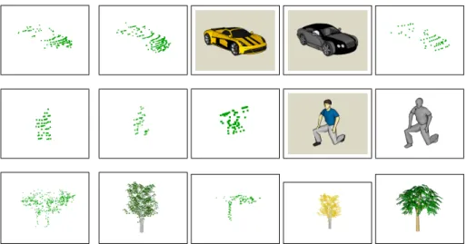
Figure 7: Exemplar matches. The leftmost column shows example segments extracted from 3D laser scans: car, person, tree (top to bottom). Second to last columns show exemplars with distance below threshold, closer exemplars are further to the left.
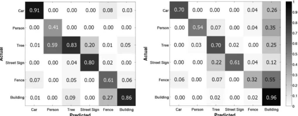
on the left, the middle and bottom row show matches for a person and tree segment, re-spectively. As can be seen, the segments extracted from the real scans are successfully matched against segments from both domains, real and 3D Warehouse. The person is mismatched with one object from the background class “other” (second row, third column). Part of the laser scan from the scene in Fig. 5 and its ground truth labeling is shown in color in Fig. 15 and in grayscale in Fig. 16 and Fig. 17. These figures also include the labeling achieved by our exemplar-based domain adaptation approach described in Section 3.2. Fig. 8 presents both the precision (column-normalized) and recall (row-normalized) confusion matrices between the six classes over all 10 scenes.
5.4
Feature Evaluation
To verify that all of the selected features contribute to the success of our approach, we also compared the performance of our approach using three different sets of fea-tures. We looked at using just bounding box dimensions and the minimum height off the ground (Dims), adding in the original, rotation-invariant spin image signatures as described in Assfalg et al. (2007) (SISO+ Dims), and adding in our3×3×3grid of
Spin Image Signatures (SISG + Dims). Fig. 9 (left) shows the precision-recall curves
obtained by the three sets of features. Once again the precision-recall curves are gen-erated by varying the probabilistic classification threshold between[0.5,1]. Although using just dimensions features or the original spin image signatures can lead to higher precision values, this comes at the cost of much lower recall.
When trained on3scans (randomly selected and repeated for10trials) using di-mensions features only, our approach achieves a maximum F-score of0.63. Using the original Spin Image Signatures and dimensions features, we achieved an F-score of
Figure 8: Confusion matrices between the six urban object classes. (left) Column-normalized precision matrix, (right) row-Column-normalized recall matrix.
Figure 9: Precision-recall curves comparing different approaches: (left) using various sets of features. (right) Using our probabilistic classification and recognition confi-dence scoring.
0.64. Finally, using our Grid Spin Image Signatures and dimensions features achieved an F-score of0.67. Due to noise and occlusions in the scans, as well as imperfect seg-mentation, the classes are not easily separable just based on bounding box dimensions alone. Also, our Grid Spin Image Signature features perform better than the original, rotation-invariant, Spin Image Signatures, justifying our modification to remove their rotation-invariance.
5.5
Classification Method Comparison
In this experiment, we compared our probabilistic classification approach to the recog-nition confidence scoring method described in Malisiewicz and Efros (2008). Letting
Ebe the list of exemplars associated with segmentz(i.e. E={e|De(z)≤1}), the
recognition confidence is defined as
s(z, E) = 1/X
e∈E
1
De(z)
The intuition here is that a lower score is better, and this is attained by having many exemplars with low distances to our segmentz. The resulting precision-recall curves are shown in Fig. 9 (right). Just as in the previous experiments, the precision-recall curve for our probabilistic classification is generated by varying the probability thresh-old between [0,1]. The precision-recall curve for recognition confidence scoring is generated by thresholding on the recognition confidence, with the label for each point being the majority label of all segments containing that point. For clarity, only the re-sult from training on5scans (randomly selected and repeated for10trials) is shown, but the trend from training on3scans is identical. As evident from the plot, the prob-abilistic classification method attains recalls between30-50percentage points above recognition confidence scoring for corresponding precision values.
5.6
Effect of Varying the
K
Parameters
Two important parameters in our domain adaptation approach areKsandKt, which
control the number of source domain and target domain exemplars to associate with each exemplar during the distance function learning process. The optimal setting for these parameters depends on a number of factors. The absolute number ofKsandKt
depends on the number of training exemplars and the amount of intra-class variation, while the ratio between the two depends on how different the source and target domains are from each other.KsandKtare determined via a grid search over possible settings
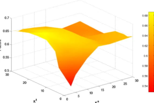
of these two parameters. Cross-validation within the training data is used to select the setting that yields the highest F-score. Fig. 10 shows a plot of how the performance of our approach varies with different settings ofKsandKt. A higher value forKt
thanKsis favored, which is to be expected since target domain exemplars tend to be
more useful than source domain exemplars. Although the approach does best when
Ksis set to be low, source domain exemplars are not completely ignored. They still
play an important role as negative exemplars. Increasing either parameter beyond a certain value leads to degradations in performance. There is a single mode around which the maximum performance is attained. The specific optimum setting was found to beKs= 3,Kt= 15.
5.7
Indoor Objects Data Set
Aside from the urban driving data set, we also evaluated our approach on an indoor objects data set, classifying objects placed on a table. As before, we manually down-loaded objects from the Google 3D Warehouse to serve as source domain exemplars. We downloaded objects from six classes: apple, book, laptop, mug, soda can, and water bottle, totaling1,700 source domain exemplars. Target domain exemplars are recorded by the prototype stereo camera and textured light projector system developed by Konolige (2010) (see Fig. 11). The system is mounted on a tripod so that it stands approximately 50cm above the table, giving it a viewpoint similar to a person sitting next to the table. The stereo camera is a Videre STOC (Stereo on a Chip) with 640x480 resolution. The textured light projector projects a fixed, red textured light pattern into the environment. Almost all of our objects have large textureless parts, such as many of the mugs, the screens of laptops, and even apples at the resolution of our camera. The
Figure 10: F-scores for different values of theKs andKt parameters used during training of the exemplar-based domain adaptation approach.
Figure 11: Stereo camera and textured light projector system.
textured light projection dramatically improves the number of correspondences found by the stereo camera in these cases. We recorded depth images of16objects from the six classes, placed on top of a table. The ground plane subtraction method described in Section 2.1 was used to remove points corresponding to the table. Each object was recorded from between 4 to 7 views, giving just under150exemplars in total. Thus, target domain exemplars are much more scarce here than in the urban data set. In this experiment, we performed leave one object out cross-validation. That is, we trained on all source domain exemplars and all target domain exemplars except those from one particular object, and evaluated on all views of that object. This was repeated with each of the16 objects being left out. Once again, theKsandKtparameters were
determined by cross-validation on the training data. This time the optimal setting was found to beKs = 20,Kt = 5. The approach used more source domain exemplars
than target domain ones, unlike in the urban data set where the reverse was true. We believe this is due both to the fact that target domain data is scarce, and because there is less difference between source and target domain exemplars; the depth images were quite accurate and the objects were placed neatly on the table with no occlusions.
Fig. 12 shows example segments and their matched exemplars in a similar manner to Fig. 7 for the urban data set, except that real exemplar point clouds are also shown as images for better visualization. The apples in the target domain set were very similar to each other, so the query apple was most closely matched to depth images of other
Figure 12: Indoor exemplar matches. The leftmost column shows example segments: apple, book, mug (top to bottom). Second to last columns show exemplars with dis-tance below threshold, closer exemplars are further to the left.
apples. The other two query objects matched to a mix of both depth images and 3D Warehouse models. Fig. 13 shows several example classification results. To create this visualization, 3D points from the depth image are classified using our approach and projected back onto the camera image. The corresponding pixels are colored based on the classification returned by the system. The first12objects are correctly classified, while the last 3 are misclassified. Notice that since the training data contains both 3D Warehouse and real exemplars in different orientations, the approach is mostly able to correctly classify the objects even though they are placed in various different orientations. However, most of the misclassifications still occur when the object is seen from oblique or unusual viewpoints, as in the last3scenes. Due to the lack of stereo correspondences and the presence of noise in the depth images, object segmentations are not perfect. Objects with dark, textureless and reflective surfaces, such as laptop screens and mugs pose the greatest challenge for the stereo camera. Nevertheless, the algorithm is still often able to correctly classify these objects. The water bottles are particularly challenging since significant portions of them are transparent and so we do not get any depth readings.
Fig. 8 presents both the precision (column-normalized) and recall (row-normalized) confusion matrices between the six classes. The system did very well distinguishing between these objects, which are quite challenging. For laptops, the stereo camera was only able to obtain 3D points from the edges because the laptop surfaces were often dark and reflective. Other objects, like apples, mugs and soda cans, can be quite similar in size and shape. Overall, our domain adaptation approach obtains a precision of 0.80, a recall of 0.75 and an F-score of 0.77. An approach trained on just target domain data obtained a precision of 0.73, a recall of 0.73 and an F-score of 0.73. The precision improvement corresponds to a>25%reduction in error.
Figure 13: Classification of indoor objects. Colors indicate labels of pixels for which depth information was available (red: apple, blue: book, orange: laptop, purple: soda can, cyan: water bottle).
6
Related Work
The problem of object recognition has been studied extensively by the computer vision community. Recently, there has been a focus on using large, web-based data sets for object and scene recognition (Li et al., 2007; Malisiewicz and Efros, 2008; Russell et al., 2008; Torralba et al., 2008) and scene completion (Hays and Efros, 2007). These techniques take a radically different approach to the computer vision problem; they tackle the complexity of the visual world by using millions of weakly labeled images along with non-parametric techniques instead of parametric, model-based approaches. The goal of our work is similar to these previous works, but these approaches have been both trained and evaluated on web-based data. In our case, we are applying the learned classifier to shape-based object recognition using data collected from a robot, which can have characteristics very different from the web-based data used to train the system.
The shape retrieval community has designed many 3D shape description features and methods for searching through a database to retrieve objects that match a given query object. Shape retrieval methods have been proposed using a number of features including 3D shape contexts (K¨ortgen et al., 2003), 3D Zernike descriptors (Novotni and Klein, 2003), and spin image signatures (Johnson and Hebert, 1999; Assfalg et al., 2007). However, the focus of this line of work is retrieving similar objects rather than the classification of the query object. Our approach uses one particular shape descriptor, spin image signatures, from this community, but with a modification that eliminates its rotation-invariance. Rotation-invariance makes sense in the context of shape retrieval if the query object can be presented in any orientation. Real-world data,
Figure 14: Precision (left) and recall (right) confusion matrices between the six indoor object classes.
however, often appears in very constrained set of orientations and so it can be a very useful cue.
Recently, several robotics research groups have also developed techniques for clas-sification tasks based on visual and laser range information (Wellington et al., 2005; Anguelov et al., 2005; Douillard et al., 2008; Triebel et al., 2007; Sapp et al., 2008). In robotics, Saxena and colleagues (Saxena et al., 2008) used synthetically generated images of objects to learn grasp points for manipulation. Their system learned good grasp points solely based on synthetic training data. Newman’s group has also done classification in maps constructed using laser range and camera data (Posner et al., 2008). Their work has thus far been concerned with terrain classification as opposed to the classification and localization of specific objects. N¨uchter et al. (2004) is an earlier work on 3D point cloud classification using Gentle AdaBoost. Although they demonstrated good results detecting office chairs in several indoor scenes, our compar-ison against a LogitBoost classifier suggests that an off-the-shelf boosting algorithm will not perform well on our data set, which contains a lot of variability in objects, orientations, and occlusions.
None of the prior work in all of these communities have, to our knowledge, explic-itly addressed differences between data from different sources as we have done with domain adaptation. The problem of combining data from different sources is a major area of research in natural language processing (Hwa, 1999; Gildea, 2001; Bacchiani and Roark, 2003; Roark and Bacchiani, 2003; Chelba and Acero, 2004). Here, text sources from very different topic domains are often combined to help classification. Several relevant techniques have been developed for transfer learning (Caruana, 1997; Dai et al., 2007) and, more recently, domain adaptation (Chelba and Acero, 2004; Jiang and Zhai, 2007; Daum´e III and Marcu, 2006; Daum´e III, 2007). In this paper, we have applied one of the state-of-the-art domain adaptation techniques from the NLP commu-nity (Daum´e III and Marcu, 2006) to the problem of 3D point cloud classification and showed that it can significantly improve performance. In addition, we also presented an alternative domain adaptation technique specific to per-exemplar distance function learning and showed that it attains slightly better performance.
7
Conclusion
The computer vision community has recently shown that using large sets of weakly labeled image data can help tremendously to deal with the complexity of the visual world. When trying to leverage large data sets to help classification tasks in robotics, one main obstacle is that data collected by a mobile robot typically has very different characteristics from data available on the World Wide Web, for example. For instance, our experiments show that simply adding Google 3D Warehouse objects to manually labeled 3D point clouds without treating them differently candecreasethe accuracy of the resulting classifier.
In this paper we presented a domain adaptation approach that overcomes this prob-lem. Our technique is based on an exemplar learning approach developed in the context of image-based classification (Malisiewicz and Efros, 2008). We showed how this ap-proach can be applied to 3D point cloud data and extended it to the domain adaptation setting. For each scene, we generate a “soup of segments” in order to generate multi-ple possible segmentations of the point cloud. The experimental results show that our domain adaptation improves the classification accuracy of the original exemplar-based approach and clearly outperforms boosting and multi-class SVM classifiers trained on the same data. The approach was additionally evaluated on a data set of indoor objects and achieved very promising results, demonstrating the effectiveness of the approach in a wide range of problem domains.
There are several areas that warrant further research. First, we classified objects solely based on shape. While adding other sensor modalities is conceptually straight-forward, we believe that the accuracy of our approach can be greatly improved by adding visual information. Here, one might be able to leverage additional data sources on the Web. In both the urban and the indoor data sets, we only distinguish between six object classes. Obviously, a realistic application will require distinguishing between many more classes. So far, we only used small sets of objects extracted from Google’s 3D Warehouse. A key question will be how to incorporate many thousands of objects for both outdoor and indoor object detection. Finally, our current implementation is not yet running in real-time. In particular, the scan segmentation and spin image feature computation take up the bulk of the time. Although the learning technique scales lin-early with the number of exemplars, the computation required at test time only involves element-wise vector multiplications, which are very fast. All of these computations are performed independently for each exemplar during training, and for each test segment during classification, much of the code can be parallelized and the technique should achieve real-time performance if implemented on a GPU. An efficient implementation and the choice of more efficient features will be a key part of future research. Over-all, we believe that this work is a promising first step toward robust many-class object recognition for mobile robots.
Acknowledgments
We would like to thank Albert Huang and the MIT DARPA Grand Challenge Team for providing us with the urban driving data. We also thank the reviewers for their
valuable comments. This work was supported in part by ONR MURI [grant number N00014-07-1-0749]; the National Science Foundation [grant number 0812671]; and by a postgraduate scholarship from the Natural Sciences and Engineering Research Coun-cil of Canada. Any opinions, findings, and conclusions or recommendations expressed in this material are those of the authors and do not necessarily reflect the views of the National Science Foundation.
References
Anguelov, D., Taskar, B., Chatalbashev, V., Koller, D., Gupta, D., Heitz, G., Ng, A., 2005. Discriminative learning of Markov random fields for segmentation of 3D scan data. In: Proc. of the IEEE Computer Society Conference on Computer Vision and Pattern Recognition (CVPR). pp. 169–176.
Assfalg, J., Bertini, M., Del Bimbo, A., Pala, P., 2007. Content-based retrieval of 3-D objects using spin image signatures. IEEE Transactions on Multimedia 9 (3), 589– 599.
Bacchiani, M., Roark, B., 2003. Unsupervised language model adaptation. In: Proceed-ings of the International Conference on Acoustics, Speech and Signal Processing. pp. 224–227.
Boser, B. E., Guyon, I. M., Vapnik, V. N., 1992. A training algorithm for optimal mar-gin classifiers. In: COLT ’92: Proceedings of the fifth annual workshop on Compu-tational learning theory. ACM, New York, NY, USA, pp. 144–152.
Caruana, R., 1997. Multitask learning: A knowledge-based source of inductive bias. Machine Learning 28, 41–48.
Chang, C.-C., Lin, C.-J., 2001. LIBSVM: a library for support vector machines. Soft-ware available athttp://www.csie.ntu.edu.tw/˜cjlin/libsvm. Chelba, C., Acero, A., July 2004. Adaptation of maximum entropy capitalizer:
Lit-tle data can help a lot. In: Lin, D., Wu, D. (Eds.), Proceedings of EMNLP 2004. Association for Computational Linguistics, Barcelona, Spain, pp. 285–292.
Comaniciu, D., Meer, P., 2002. Mean shift: A robust approach toward feature space analysis. IEEE Transactions on Pattern Analysis and Machine Intelligence (PAMI) 24 (5), 603–619.
Dai, W., Yang, Q., Xue, G., Yu, Y., 2007. Boosting for transfer learning. In: Proc. of the International Conference on Machine Learning (ICML). pp. 193–200.
Daum´e III, H., 2007. Frustratingly easy domain adaptation. In: Proc. of the Annual Meeting of the Association for Computational Linguistics (ACL). pp. 256–263. Daum´e III, H., Marcu, D., 2006. Domain adaptation for statistical classifiers. Journal
Douillard, B., Fox, D., Ramos, F., 2008. Laser and vision based outdoor object map-ping. In: Proc. of Robotics: Science and Systems (RSS). pp. 9–16.
Fischler, M. A., Bolles, R. C., 1981. Random sample consensus: a paradigm for model fitting with applications to image analysis and automated cartography. Commun. ACM 24 (6), 381–395.
Friedman, J., Hastie, T., Tibshirani, R., 2000. Additive logistic regression: A statistical view of boosting. The Annals of Statistics 28 (2), 337–407.
Gildea, D., 2001. Corpus variation and parser performance. In: Lee, L., Harman, D. (Eds.), Proceedings of the 2001 Conference on Empirical Methods in Natural Lan-guage Processing. pp. 167–202.
Google, 2008. 3D Warehouse. Software available athttp://sketchup.google. com/3dwarehouse/.
Hall, M., Frank, E., Holmes, G., Pfahringer, B., Reutemann, P., Witten, I. H., 2009. The weka data mining software: an update. SIGKDD Explor. Newsl. 11 (1), 10–18. Hays, J., Efros, A., 2007. Scene completion using millions of photographs. ACM
Transactions on Graphics (Proc. of SIGGRAPH) 26 (3), 4.
Hwa, R., 1999. Supervised grammar induction using training data with limited con-stituent information. In: In Proceedings of the 37th Annual Meeting of the ACL. pp. 73–79.
Jiang, J., Zhai, C., 2007. Instance weighting for domain adaptation in NLP. In: Proc. of the Annual Meeting of the Association for Computational Linguistics (ACL). pp. 264–271.
Johnson, A., Hebert, M., 1999. Using spin images for efficient object recognition in cluttered 3D scenes. IEEE Transactions on Pattern Analysis and Machine Intelli-gence (PAMI) 21 (5), 433–449.
Keerthi, S. S., Chapelle, O., DeCoste, D., 2006. Building support vector machines with reduced classifier complexity. J. Mach. Learn. Res. 7, 1493–1515.
Konolige, K., 2010. Projected texture stereo. In: Proc. of the IEEE International Con-ference on Robotics & Automation (ICRA). In-press.
K¨ortgen, M., Park, G. J., Novotni, M., Klein, R., Apr. 2003. 3d shape matching with 3d shape contexts. In: The 7th Central European Seminar on Computer Graphics. pp. 1–12.
Li, L.-J., Wang, G., Fei-Fei., L., 2007. Optimol: automatic object picture collection via incremental model learning. In: IEEE Computer Vision and Pattern Recognition (CVPR). pp. 1–8.
Malisiewicz, T., Efros, A., 2007. Improving spatial support for objects via multiple segmentations. In: Proc. of the British Machine Vision Conference. pp. 1–10.
Malisiewicz, T., Efros, A., 2008. Recognition by association via learning per-examplar distances. In: Proc. of the IEEE Computer Society Conference on Computer Vision and Pattern Recognition (CVPR). pp. 1–8.
Novotni, M., Klein, R., 2003. 3d zernike descriptors for content based shape retrieval. In: SM ’03: Proceedings of the eighth ACM symposium on Solid modeling and applications. ACM, New York, NY, USA, pp. 216–225.
N¨uchter, A., Surmann, H., Hertzberg, J., 2004. Automatic classification of objects in 3d laser range scans. In: In Proc. 8th Conf. on Intelligent Autonomous Systems, pages 963 ??970. IOS Press, pp. 963–970.
Posner, I., Cummins, M., Newman, P., 2008. Fast probabilistic labeling of city maps. In: Proc. of Robotics: Science and Systems (RSS). pp. 17–24.
Roark, B., Bacchiani, M., 2003. Supervised and unsupervised pcfg adaptation to novel domains. In: NAACL ’03: Proceedings of the 2003 Conference of the North Amer-ican Chapter of the Association for Computational Linguistics on Human Language Technology. Association for Computational Linguistics, Morristown, NJ, USA, pp. 126–133.
Russell, B., Torralba, A. Murphy, K., Freeman, W., 2008. Labelme: a database and web-based tool for image annotation. International Journal of Computer Vision 77 (1-3).
Sapp, B., Saxena, A., Ng, A., 2008. A fast data collection and augmentation procedure for object recognition. In: Proc. of the National Conference on Artificial Intelligence (AAAI). pp. 1402–1408.
Saxena, A., Driemeyer, J., Ng, A., 2008. Robotic grasping of novel objects using vi-sion. International Journal of Robotics Research 27 (2), 157–173.
Shi, J., Malik, J., 2000. Normalized cuts and image segmentation. IEEE Transactions on Pattern Analysis and Machine Intelligence (PAMI) 22 (8), 731–737.
Shilane, P., Min, P., Kazhdan, M., Funkhouser, T., 2004. The princeton shape bench-mark. In: Shape Modeling International. pp. 167–178.
Torralba, A., Fergus, R., Freeman, W., 2008. 80 million tiny images: a large dataset for non-parametric object and scene recognition. IEEE Transactions on Pattern Analysis and Machine Intelligence (PAMI) 30 (11), 1958–1970.
Triebel, R., Schmidt, R., Martinez Mozos, O., Burgard, W., 2007. Instance-based amn classification for improved object recognition in 2d and 3d laser range data. In: Proc. of the International Joint Conference on Artificial Intelligence (IJCAI). pp. 2225–2230.
van Rijsbergen, C., 1979. Information Retrieval, 2nd ed. Butterworths, London. Wellington, C., Courville, A., Stentz, T., 2005. Interacting Markov random fields for
simultaneous terrain modeling and obstacle detection. In: Proc. of Robotics: Science and Systems (RSS). pp. 1–8.
Figure 15: (top) Ground truth classification for part of a 3D laser scan. Colors indicate ground plane (cyan) and object types (green: tree, blue: car, yellow: street sign, pur-ple: person, red: building, grey: other, white: not classified). (bottom) Classification achieved by our approach. As can be seen, most of the objects are classified correctly. The street signs in the back and the car near the center are not labeled since they are
Figure 16: Labeling results for individual object classes. Black points in the left row panels show ground truth points for person, tree, and building (top to bottom). Right row shows labels by our approach. All three classes are perfectly detected in this scene. The tree labeled by our approach in the upper right portion of the scene strongly resembles a tree and may be a mislabeling of the ground truth.
Figure 17: Labeling results for individual object classes (continued). Black points in the left row panels show ground truth points for car and street sign (top to bottom). Right row shows labels by our approach. There are some false negatives for these two classes.