Planning and Scheduling Transportation Vehicle Fleet in a Congested Traffic Environment

Planning and Scheduling

Transportation Vehicle fleet in a

Congested Traffic Environment

LAOUCINE KERBACHE

AND TOM VAN WOENSEL

1 _{HEC SCHOOL OF MANAGEMENT, PARIS, FRANCE.}

2 _{EINDHOVEN UNIVERSITY OF TECHNOLOGY, THE NETHERLANDS.}

Transportation is a main component of supply chain competitiveness since it plays a major role in the inbound, inter-facility, and outbound logistics. In this context, assigning and scheduling vehicle routing is a crucial management problem. Despite numerous publications dealing with efficient scheduling methods for vehicle routing, very few addressed the inherent stochastic nature of travel times in this problem. In this paper, a vehicle routing problem with time windows and stochastic travel times due to potential traffic congestion is considered. The approach developed introduces mainly the traffic congestion component based on queueing theory. This is an innovative modeling scheme to capture the stochastic behavior of travel times. A case study is used both to illustrate the appropriateness of the approach as well as to show that time-independent solutions are often unrealistic within a congested traffic environment which is often the case on the European road networks.

1. Introduction

Transportation is a main component of supply chain competitiveness since it plays a major role in the inbound, inter-facility, and outbound logistics. Transportation costs represent approximately 40 to 50 percent of total logistics and 4 to 10 percent of the product selling price for many companies (Coyle et al., 1996). Transportation decisions directly affect the total logistic costs. The passage of the transportation deregulation acts

in the 1980's in the USA and in the 1990's in the EU drastically changed the business climate within which the transportation managers operate. Within the EU, the competition is becoming intense between transporters since they often operate at transnational levels and must provide higher levels of service with lower costs to meet the various needs of customers. In this context, assigning, scheduling and routing the fleet of a transportation company is a crucial management problem.

Providing non dominated vehicle routing planning schedules is a very hard combinatorial problem. Yet, the manager must rely on management techniques to identify and solve transportation problems and to provide the company with a competitive advantage in the marketplace. Despite numerous publications dealing with efficient scheduling methods for vehicle routing, very few addressed the inherent stochastic nature of this problem. Most research in this area has focused on dynamic routing and scheduling that considers the variation in customer demands. However, there has been limited research on routing and scheduling with probabilistic travel times.

Only few researchers (e.g. van Woensel et al., 2003; Ichoua et al., 2003; Malandraki and Daskin, 1992; Hill and Benton, 1992; Malandraki and Dial, 1996) have dealt with time dependent travel times. Further, for stochastic travel times, the problem is much more complex and the literature is virtually nonexistent. For a review, we refer the reader to our previous paper (van Woensel and Kerbache, 2004).

In this paper, we consider a vehicle routing problem with stochastic travel times due to potential traffic congestion. The approach developed introduces mainly the traffic congestion component that is modeled through a queueing networks approach and combined with an Ant Colony Optimization heuristic. For instance, the stochastic nature of travel times is captured using queueing theory applied to traffic flows (see e.g. Van Woensel, 2003). An application and preliminary results will be presented along with a discussion of potential unfeasibility of many of the published results to test problems if travel times were appropriately modeled.

This paper is organized as follows: in section 2, some background on the vehicle routing problems is presented. Section 3 deals with a classification of these problems and their corresponding literature review.

Section 4 is devoted to the modeling and determination of the travel time distribution. Section 5 addresses the ant colony approach used as an optimization methodology to cope with the vehicle routing. In section 6, computational results are presented based on some standard datasets. Finally, conclusions are presented in section 7.

2. Background on vehicle routing problems

The vehicle routing problem (VRP) can be described as a more general version of the well-known traveling salesman problem (TSP). The VRP aims to construct a set of shortest routes for a fleet of vehicles of fixed capacity. Each customer is visited exactly once by one vehicle which delivers the demanded amount of goods. Each route has to start and end at a depot, and the sum of the visited customers demands, on a route, must not exceed the capacity of the vehicle. Another common constraint is that the customer may specify time intervals for deliveries. This additional restriction leads to what is known as the vehicle routing problem with time windows (VRPTW). These time windows are referred to as either soft or hard depending on whether they can be violated or not (Laporte, 1992).

The VRPTW is known to be an NP-Hard combinatorial problem and it is often solved by heuristics except for very small problems. Many heuristics developed for the VRPTW are actually derivations of methods used for the VRP. We mention the nearest neighbor algorithms, the insertion algorithms, and the tour improvement procedures. These can be used for the VRPTW with some minor modifications. However, due to stronger constraints, the feasibility of the solution must be checked (Laporte, 1992). Nevertheless, there are some algorithms that are specifically developed for the VRPTW. These have proved useful in a wide range of practical size VRPTW (Desrochers et al. 1992). Most of the best performing heuristics use a two-phase approach. First, a construction heuristic is used to generate a feasible initial solution. During the second phase, an iterative improvement heuristic is applied to the initial solution. Construction heuristics build routes sequentially or in parallel, and improvement heuristics are used to obtain higher quality solutions by

trying modifications to the incumbent solution. Meta-heuristics can guide the construction heuristics to generate a diversified set of initial solutions and help improvement heuristics to escape local optima.

In practice, there are many variations to the VRPTW. Some have different delivery situations while others have various characteristics of the transportation system itself. For instance, the dial-a-ride problem consists of transporting items from their specific origins to their respective destinations. This means that there is no notion of a central depot since this changes depending on the item (Osman, 1993). Other variations include characteristics such as: one or many depots, a fleet of one or several vehicles with homogeneous or heterogeneous capacities, one or different goods to be delivered, etc.

In the VRPTW considered in this paper, we assume that there is only one depot from where the routes start and end for each vehicle, a homogeneous fleet consisting of several vehicles with fixed capacity, while each customer’s demand is pre-determined. Formally, the vehicle routing problem can be represented by a complete weighted graph

G=(V,A,c) where V={0,1,...,n} is a set of vertices and A={(i,j):i≠j} is a set of arcs. The vertex 0 denotes the depot, the other vertices of V represent cities or customers. The non-negative weights c which are associated with each arc (i,j) represent the cost (distance, travel time or travel cost) between i and j. For each customer, a non-negative demand qi and a

non-negative service time δi is given (δ0=0 and q0=0). The aim is then to find

the minimum cost vehicle routes where the following conditions hold: Every customer is visited exactly once by exactly one vehicle All vehicle routes start and end at the depot

Every vehicle route has a total demand not exceeding the vehicle capacity Q

Every vehicle route has a total route length not exceeding the maximum length L

Every customer i has a predetermined time window [tli,tui] and

tli<tui in which he wants to be delivered

If it seems reasonable to assume that the service time at each vertex (customer) is known in advance, it is definitely not the case for the travel time between two vertices. In fact, the travel times are the result of a stochastic process related to traffic congestion. Clearly, travel times depend greatly on the different number of vehicles occupying the road and on their speeds. This section gives a comprehensive classification of vehicle routing problems based on the characteristics of travel times.

Time-Independent Routing Problems

The time-independent routing problem can be referred to as the standard case. In this instance, most of these models assume that all the characteristics are independent of time of the day. Therefore, these models are far from real-world applications since traffic congestion affects significantly travel time on the used road network. Laporte (1992) surveyed the main research results related to the time-independent vehicle routing problem. Both exact and heuristic methods were developed depending on the complexity of the problems addressed. He classified exact algorithms into three categories: direct tree search methods, dynamic programming and integer programming. For larger (more realistic) and complex problems, one needs to resort to heuristics for any solutions. In the literature, the time-independent routing problem is modeled differently depending on whether the parameters are deterministic or stochastic.

Deterministic Time-Independent Routing Problems

Most of the heuristics for these types of problems are derivations of methods developed for the TSP. They are basically classified as follows: constructive heuristics [e.g. the savings algorithm of Clarke and Wright (1964), and Gillet and Miller (1974)], two-step heuristics [e.g. cluster-first-route-second methods, route-first-cluster-second methods, Christofides-Mingozzi-Toth two-phase algorithm, Christofides et al. (1989)], incomplete optimization, local search heuristics [sweep algorithm, Gillet (1974)], meta-heuristics [tabu search algorithm by Gendreau, Hertz and Laporte, (1992)], and space filling curves.

Stochastic Time-Independent Routing Problems

These problems arise whenever some elements of the deterministic routing problems are assumed to be random. Common examples are stochastic demands, set of customers to be visited not known with certainty (Gendreau et al., 1996), etc. Since they combine the characteristics of stochastic and integer programming, these type of problems are often seen as computationally intractable. Stochastic VRPs can be modeled either as a chance constrained program (CCP) or as a stochastic program with recourse (SPR). In CCPs, one seeks a first stage solution for which the probability of failure is constrained to be below a certain threshold. A CCP solution does not take into account the cost of corrective actions in case of failure. In SPRs, the aim is to determine a first stage solution that minimizes the expected cost of the second stage solution: this cost is made up of the cost of the first stage solution, plus the expected net cost of recourse (Gendreau et al., 1996).

Time-Dependent Routing Problems

The motivation for using time-dependent models is that in reality the vehicles operate in a traffic network that may be congested depending on the time of the day. In the time-dependent routing models, the non-negative weight c assigned to each arc (i,j) is associated with a variable travel time between i and j and thus, the cost involved with traversing an arc will change over time. This is not the case in the time-independent routing models since the cost is associated with distance. The literature related to vehicle routing with time-dependent travel times is rather scarce (Ichoua et al. , 2003, Malandraki and Daskin, 1992, Hill and Benton, 1992, Malandraki and Dial, 1996, Kenyon and Morton, 2003). In general, the time-dependent travel times can be either considered deterministic or stochastic.

Deterministic Time-Dependent Routing Problems

In the deterministic case, the travel times are known in advance and plugged in the solution approach depending upon the period of the day. The travel times are then a function of the distance and the mean speed.

For instance, Ichoua et al. (2003) consider three distinct time periods: the first and third periods stand for the morning and evening rush hours, respectively while the second period corresponds to the middle part of the day. They also considered three different types of road links. This approach has been implemented using a parallel tabu search approach developed by Taillard et al. (1995). As the different speeds are known in advance (and thus, the travel times too), no recourse procedure is needed after the first stage solution. A similar approach is used by Fleishmann et al. (2004).

Stochastic Time-Dependent Routing Problems

In the stochastic time-dependent models, the solution procedure takes into account the stochastic nature of the travel times. Travel times are now the result of taking into account not only the mean travel time but also the travel time distribution. As the travel time distribution is derived from the speed distribution and from the known distances, this approach requires realistic speed distributions. However, in practice neither the travel time nor the speed distributions are available in closed form. Our research paper is an incursion in this almost unexplored domain.

4. Characterization of the travel time distribution using

queueing theory

In the time-dependent VRP, the key issue is the computation of the travel times on arcs dependent upon the time period. In general, the travel time from city i to city j during time period p, is determined as follows:

p ij ij p ij v d T = (1)

Hence, to determine the travel time on arc (i,j) one needs information on the length of (i,j) and on the travel speed on that arc in time bucket p: . The distance is already available in the time-independent VRP models, but the speed still needs to be specified. In this paper, the speeds are obtained using queueing models for traffic flows (Vandaele et al., 2000 and Heidemann, 1997).

p ij v

In what follows, the approach developed for the characterization of the travel time distribution is described in detail. First, the queueing approach to determine the time-dependent travel times is explained. Second, the specific calculations of the travel times taking into account the different time periods that a vehicle might cross are discussed.

Queueing approach

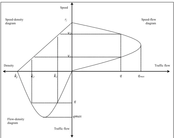
It is often observed that the speed for a certain time period tends to be reproduced whenever the same flow is observed. Based on this observation, it seems reasonable to postulate that, if traffic conditions on a given road are stationary, there should be a relationship between flow, speed, and density. This relationship results in the concept of speed-flow-density diagrams. These diagrams describe the interdependence of traffic flow (q), density (k) and speed (v). The seminal work on speed-flow diagrams was the paper by Greenshields in 1935.

Using well-known formulas of queueing models, these speed-flow-density diagrams can be constructed (Figure 1). Figure 1 illustrates that, although every speed v corresponds with one traffic flow q, the reverse is not true. There are two speeds for every traffic flow: an upper branch (v₂) where speed decreases as flow increases and a lower branch (v₁) where speed increases. Intuitively it is clear that, as the flow moves from 0 (at free flow speed vf to qmax, congestion increases but the flow rises because the decline in speed is over-compensated by the higher traffic density. If traffic tends to grow past qmax, flow falls again because the decline in speed more than offsets the additional vehicle numbers, further increasing congestion (Daganzo, 1997). The flow-density diagram and the speed-density diagrams are an equivalent representation and can be interpreted in the same way.

Figure 1: The relations between the speed-flow, the speed-density, and the flow-density diagrams qmax q kj Traffic flow k1 k2 v2 v1 q qmax vf Traffic flow Speed Speed-flow diagram Speed-density diagram Flow-density diagram Density

Traditionally, these speed-flow-density diagrams are modeled empirically: speed and flow data are collected for a specific road and econometrically fitted into curves (Daganzo, 1997). This traditional approach is limited in terms of predictive power and sensitivity analysis. Vandaele et al. (2000) and Heidemann (1997) showed that queueing models can also be used to explain uninterrupted traffic flows and thus offering a more practical approach, useful for sensitivity analysis, forecasts, etc. Jain and Smith (1997) describe in their paper a state-dependent M/G/C/C queueing model for traffic flows. Part of their logic is used to extend our queueing models to state-dependent ones. Also a lot of research is done on a travel time-flow model originating from Davidson (1978). The model is based on some concepts of queueing

theory but a direct derivation has not been clearly demonstrated (Akçelik, 1991 and Akcelik, 1996).

In a queueing approach to traffic flow analysis, roads are subdivided into segments, with length equal to the minimal space needed by one vehicle on that road (Figure 2). Define kj as the maximum traffic density (i.e. maximum number of cars on a road segment). This segment length is then equal to 1/ kj and matches the minimal space needed by one vehicle on that road. Each road segment is then considered as a service station, in which vehicles arrive at a certain rate λ and get served at another rate µ (Vandaele et al., 2000; Van Woensel et al., 2001; Heidemann, 1996).

Figure 2: Queueing representation of traffic flows

µ

λ

Queue Service Station (1/C)

Vandaele et al. (2000) developed different queueing models1. The M/M/1 queueing model (exponential arrival and service rates) is considered as a base case, but due to its specific assumptions regarding the arrival and service processes, it is not useful to describe real-life situations. Relaxing the specifications for the service process of the M/M/1 queueing model, leads to the M/G/1 queueing model (generally distributed service rates). Relaxing both assumptions for the arrival and service processes results in the GI/G/m queueing model. Moreover, following Jain and Smith (1997), a special case of the GI/G/m queueing model is derived: a state dependent GI/G/m queueing model. This model assumes that the service rate is a (linear, exponential, etc.) function of the traffic flow. In this case, vehicles are served at a certain rate which depends upon the number of vehicles already on the road (Vandaele et al.,

1_{In this paper, queueing models are refered to using the Kendall notation, consisting of}

several symbols - e.g. M/G/1. The first symbol is shorthand for the distribution of inter-arrival times, the second for the distribution of service times and the last one indicates the number of servers in the system.

2000). Vandaele et al. (2000) and Heidemann (1997) showed that the speed v can be calculated by dividing the length of the road segment by the total time in the system (W). The total time in the system W is different depending upon the queueing model used and can be obtained as the sum of the waiting time Wq and the service time Wp, or: W = Wq + Wp.

For the GI/G/m queueing models, no exact solutions for the waiting times are available and one must rely on approximations. Of the available, we mention here three approximations. The Kramer-Lagenbach-Belz (KLB) approximation is widely used but it is limited to single servers only. To cope with multiple lanes, the Kingman approximation and the Whitt (W) approximations with multiple servers are used. We opted for the Whitt approximations because they have been shown to perform better in a wide range of cases (Whitt, 1993).

In general, formula (1) can be rewritten in the following basic form: Ω + = 1 f v v ₍₂₎

Formula (2) shows that the speed is only equal to the free flow speed v_f if the factor Ω is zero. For positive values of Ω, _f is divided by a number strictly larger than 1 and speed is reduced. The factor Ω is thus the influence of congestion on speed. High congestion (reflected in a high Ω) leads to lower speeds than the maximum. The factor Ω is a function of a number of parameters depending upon the queueing model chosen: the traffic intensity r, the coefficient of variation of service times

c

v

s and coefficient of variation of inter-arrival times ca, the jam density kj

and the free flow speed vf. High coefficients of variation or a high traffic intensity will lead to a value of Ω strictly larger than zero. Actions to increase speed (or decrease travel time) should then be focused on decreasing the variability or on influencing the traffic intensity, for example by manipulating the arrivals (arrival management and ramp metering).

In the remainder of this paper, the GI/G/m queueing models are applied using the Whitt approximations which, as mentioned earlier, have proven their robustness and relative accuracy. Consequently, one has four

parameters that can be influenced: the coefficient of variation of service times cs and coefficient of variation of inter-arrival times ca, the jam

density kj and the free flow speed vf. In practice, the jam density and the free flow speed is fixed for a given arc (i,j), leaving only the coefficients of variation to represent the traffic conditions (e.g., bad weather, etc.). The major strength of using the queueing models, is that given the flow q, the speed can easily be obtained in an analytical way. The flow q is a parameter that can be determined empirically, allowing to determine realistic velocity profiles as a function of time.

For a more detailed discussion of the queueing models and their results, the interested reader is referred to Vandaele et al. (2000) and Van Woensel et al. (2002).

Computing travel times

To compute the travel time, one should note that in the time-dependent case, the travel speeds are no longer constant over the entire length of the arc. More specifically, one has to take into account the change of the travel speed when the vehicle crosses the boundary between two consecutive time periods. For example, the speed changes when going from time period p to time period (p+1) from p to .

ij

v p+1

ij v

In this paper, the time horizon is discretized into P time periods of equal length ∆p with a different travel speed associated to each time period p (1≤p≤P). The travel speeds are obtained using the above discussed queueing models for traffic flows. Formally, the travel time T_ij

going from customer i to customer j, starting at some time p₀, is defined by the following formula:

∫

With denoting the speed in time period p and _ij the distance traveled. Solving this integral for and making using of the discrete time horizon, results in:

p ij v d ij T ) ... ( 0 0 1 0 ( 2) last ij k p ij p ij p ij v v v v p dij=∆ ϕ + + + + + − +φ

Rewriting as a function of the time slices, gives: last

first

ij p k p p

With ∆pfirst the first time zone which contains p₀ and ∆plast the last

time zone used to cover the distance dij and k the total number of time

slices needed (which is a function of the different speeds). The expected travel time is thus the sum of the following components:

The fraction of travel time still available in the first time zone, given by (ϕ∆pfirst) with pfirst the first time zone which contains p₀

and ϕ the fraction parameter (0≤ϕ≤1).

The travel times of the (k-2) intermediate time zones passed: (k-2)

∆p.

The fraction of the travel time in the last time zone, given by (φ∆plast), with φ the fraction parameter (0≤φ≤1).

Using this procedure, the travel time Tij from customer i to

customer j, starting at time p₀ can easily be determined based on the distance dij and the speed for the different time periods p obtained

from the queueing models given a certain flow q in that time period. p

ij v

The variance of the travel time

In this section, an expression for the variance of the travel time is derived. Again, using the queueing approach to traffic flow (Van Woensel, 2003) the variance can be obtained in a closed form. For each time period p, the variance of the travel time can be determined as follows:

The distance from i to j, dij and the jam density of the road kj are

assumed to be known. The variance of the total time in the system W, can be obtained using the two moment approximations from Whitt. As there is no exact form for the variance of the waiting time, one needs to rely on approximations to obtain the variance of the waiting time (Whitt, 1993). These approximations have already proven their value and usability in production management (Vandaele, 1996; Whitt, 1993; and others). Whitt describes an approximation for the variance of the waiting time for the

) ( ) ( ) ( ) ( 2 2 p j ij p ij p ij ij p ij W Var k d T v d Var T = = Var Var

case when expected waiting time is known (either exact or approximated). Only the results necessary for the analysis of the variance of the waiting time are presented here. For a detailed discussion, the reader is referred to Whitt (1993). The approximation has the following general form:

2 2 2 2 2 ) (_Wp _{WqcW cskjvf} Var _q with: c + =

Wq² the squared coefficient of variation of the waiting times.

The specific approximations for this variable are out of the scope for this paper, but can be found in Whitt (1993).

Illustration of the travel time results

An illustration of the travel time results is shown in figure 3. If one wants to go from customer i to j, the vehicle follows its way and will need

6 time zones to get to its destination. It will leave somewhere in time zone

1 (leaving time i or LTi) and will arrive in time zone 6 (arrival time ATj) at

customer j. For each time zone, the bold line represents the distance traveled in that time zone. Consequently, the slope of the line is the speed, which is the result of the queueing models.

The overall travel time from i to j is then the number of time zones passed in full (e.g. here 4 time zones: 2-5) and part of the first time zone (e.g. 1) and the last time zone (e.g. 6). In the same way, the overall variance of the travel time from i to j can be obtained. It is then assumed that there are no overflow effects over the different time zones, i.e. the covariance component is assumed to be zero.

5. Ant Colony Optimization

In this section, the integration of the time-dependent travel times in the Ant Colony Optimization (ACO) approach for the VRP is discussed. The ACO algorithm is a stochastic optimization algorithm specifically intended to solve discrete optimization problems, like the above-described VRP. The inspiration of the ACO algorithm comes from the observation of the trail laying and the trail following behavior of a real ant species (Linepithaeme humile). As the ants move in search for food, they deposit an aromatic essence called pheromone on the ground. The amount deposited generally depends upon the quality of food sources found. Other ants, observing the pheromone are more likely to follow the pheromone trail, with a bias towards stronger trails. As such, the pheromone trails reflect the memory of the ant population and over time, trails leading to good food sources will be reinforced while paths leading to remote sources will be abandoned (Corne, Dorigo and Glover, 2002).

The above behavior of real ants is translated in the ACO metaheuristic. Artificial ants construct solutions for a given combinatorial optimization problem by taking a number of decisions probabilistically. In a first stage, these decisions are based on local information only (e.g. an heuristic rule). Gradually a trail emerges as the ants lay artificial pheromone on the paths they followed. This pheromone dropping is dependent upon the quality of the solution they found: poor solutions get less pheromone than better ones. The other ants are then guided in their decision making not only by the local information but also by the collective memory based on the pheromone. Over time, paths with a high pheromone concentration will be reinforced and the artificial ants are guided to promising regions of the search space.

I Initialization II For Imax iterations do:

(a) For each ant k=1,...,m generate a new solution (b) Daemon actions to improve the solution

(c) Update the pheromone trails

Table 2: Pseudo-code for the ACO metaheuristic

In table 2, the ACO meta-heuristic is described in pseudo-code. After initializing (where the pheromone level is set to a small value next to zero), the heuristic starts building routes for a certain prefixed number of iterations Imax. Each step in the iterations part of the ACO meta-heuristic, is discussed in more detail below.

Generating new solutions

Ants start out in a randomly chosen first city. Next, they successively choose new cities to visit until all cities are visited. The depot is selected whenever the vehicle capacity or the total route length is exceeded. In this case, a new route starting at the depot is started. The selection of a new city to visit is based upon a probabilistic decision rule taking into account two aspects: how good was the choice of that city in the past and how promising is the choice of that city at this moment. The first aspect is information stored in the pheromone trails associated with each arc (i,j), i.e. memory from previous iterations. The second aspect is called visibility which stores the local heuristic information (Bullnheimer et al., 1999).

Ants probabilistically choose their next city based on the following probability distribution:

[ ] [ ] [ ]

[ ]

[ ]

[ ] [ ] [ ]

[ ]

[ ]

otherwise

pij

j

if

p

,

0

_

,

=

Λ

∈

=

∑

ψ

κ

ν

η

τ

ψ

κ

ν

η

τ

The above probability distribution combines both memory and visibility aspects. It is biased by the parameters α, β, ϱ, λ and ϖ that determine the relative influence of the pheromone at the trails and the different parts of the visibility (

p ij τ

[ ][ ]

[ ]

[ ]

η , , , ) respectively. Note that

in the time-dependent case, the pheromone level and the visibility components have an extra time dimension p based on the different time zones. The various variables are now discussed in more detail.

The first variable refers to the time-dependent pheromone level at arc (i,j). This variable gets updated for each iteration and will be a representation of the quality of the solutions found in the past. The pheromone updating procedure is discussed later.

p ij

τ

The above function is extended with VRP specific information. First, a function of the mean travel time between i and j is added:

p ij p ij T 1 = η

It should be clear that arcs with a smaller expected travel time are favored over long expected travel times based on the above function. Note also that this function is the equivalent of the one described in Bullnheimer et al. (199a) but now expressed in travel time instead of speed.

Thirdly, the variable gives an indication of the variance of the travel time on arc (i,j) and is defined as:

p ij ν

( )

Consequently, arcs with less variability are preferred over arcs with higher variability.

Moreover, a parameter κ_ij being the degree of capacity utilization is introduced. The idea is that selecting a city that leads to a higher degree of utilization of the vehicle, is to be preferred. The degree of capacity utilization κ_ij (the vehicle is in city i and has used up so far a capacity of

Qi and wants to go to city j), is defined as follows (Bullnheimer, et al.

1996): Q q Q_{i j} ij + = κ

The last variable is a time windows variable indicating to what degree the (hard or soft) time window is met. In the case of hard time windows, is either equal to 1 (if the hard time window at customer j is met) or equal to 0 (if the hard time window at customer j is not met). This results always in a probability zero for customer j if the time window cannot be met. In the extreme case, this will result in as many routes as there are customers, i.e. each customer is incorporated in a single route.

p ij ψ p ij ψ

For soft time windows, the variable can have all values between 0 and 1, with a value close to 0 a strong probability that the time window will not be met and a value of 1 a strong probability that the time window will be met.

p ij

ψ

Daemon actions to improve the solutions

After an artificial ant k has constructed a feasible solution, there are then two possible actions to take: either the pheromone trails get updated immediately using these first solutions found or the solutions are first improved using a daemon action (improvement step). In the general ACO meta-heuristic, the daemon actions are optional, but experiments have shown (Bullnheimer et al., 1999b; Bullnheimer et al., 1999a) that in the case of VRPTW, the daemon actions greatly improve the solution quality and the speed of convergence.

At the end of the solution generation, all routes are checked as before for 2-optimality and are improved if possible. A route is 2-optimal if it is not possible anymore to improve the route by exchanging two arcs. Unlike in the deterministic VRPTW where the gain is calculated based on distances, in the time-dependent VRPTW, the gain is calculated in terms of travel time.

In addition, extra improvement heuristics are performed taking into account explicitly the time-dependent nature of the problem. First, all the different subtours that make up a complete VRPTW solution, are checked whether it would be advantageous in terms of travel time to break up the sub-route in two parts by adding the depot. This procedure is repeated until no more improvements can be realized or if the maximum number of

trucks is exceeded. Secondly, all starting times of the different subtours that make up a complete VRPTW solution, are shifted in time to evaluate the effect of the start time on the total travel time. In case of improvement, the starting time of the associated subtour is updated. The rationale behind this optimization is that in a dynamic reality, a truck can decide to leave earlier or later to avoid periods of high congestion.

Of course, all daemon actions described here have an extra constraint: the action should result in an improvement in terms of travel time and lateness.

Update the pheromone trails

After the route construction and the improvement of these original routes, the pheromone is deposited on the different links depending upon the solution quality. The solution quality is the objective value obtained which equals the total accumulated lateness of the route for ant k defined as Lk. For each arc (i,j) part of the route used by ant k, the pheromone is

increased by∆τijk=1/(Lk). Using this updating rule, more costly routes in

terms of lateness will increase the pheromone levels on the arcs less than lower cost routes.

In addition to the pheromone updates using the routes of all the ants, all arcs belonging to the so far best solution defined as L* are emphasized as if σ ants (the so-called elitist ants) had used them. One elitist ant increased the pheromone level by an amount ∆τij*=1/(L*) if arc

(i,j) is part of the best route so far (Bullnheimer et al 199a).

In a last step, part of the existing pheromone trails evaporates with a factor (1-ρ), ρ being the trail persistence and 0≤ρ≤1. Pheromone evaporation is needed to avoid a too rapid convergence of the algorithm towards a sub-optimal region. It implements a form of forgetting, making the exploration of new areas of the search space possible.

Summarizing, the pheromone update after iteration t is done as follows: * 1 1 ij k ij m k t ij t ij ρτ τ σ τ τ = +

∑

Where ρ being the trail persistence and 0≤ρ≤1, σ the number of elitist ants, ∆τijk ≠0 if arc (i,j) is used by ant k and ∆τij* ≠0 if arc (i,j) is

used by the ant with the best solution so far. Using this pheromone update rule, arcs used by many ants and which are contained in shorter tours will receive more pheromone and will be more likely to be chosen in future iterations of the algorithm (Dorigo and Stutzl, 2002).

Justification of the ACO approach

This approach has been successfully applied to a number of combinatorial optimization problems such as the Graph Coloring Problem, the Traveling Salesman Problem, the Quadratic Assignment Problem, the Vehicle Routing problem, and the Vehicle Routing Problem with Time Windows (see e.g. Dorigo et al., 2002 for references).

The main feature of ACO is the ease with which various extensions to the basic version could be introduced. Further, Bullnheimer et al. (1999) showed that the ant colony optimization approach is competitive compared to other metaheuristics such as Tabu Search, Simulated Annealing and genetic algorithms. In their experience, the ACO approach gave results that are within an average deviation of less than 1.5% over the best known solutions (also on the Augerat sets – which is the set used here). In addition, the authors found that in general the ACO approach could compete with the other different metaheuristics regarding the speed and the quality of the solutions. All the different local search heuristics (such as simulated annealing and tabu search) rely on the concept of neighborhood and neighborhood solutions. Unfortunately, defining these neighborhoods is not a very straightforward task. The ACO approach overcomes this disadvantage by not relying on the neighborhood concept. In fact, as seen in the algorithmic description above, it generates new solutions at each new iteration. Further, the ACO approach has an advantage over genetic algorithms since it is not necessary to find the appropriate crossover operators. Lastly, positive feedback within the population can still be exploited in the ACO approach (Bullnheimer et al., 1999).

Computation time is an important issue for all the heuristics developed to tackle NP-Hard problems like the VRPTW. In our case,

computation is irrelevant for ACO since the heuristic runs for a fixed pre-specified number of iterations. Each iteration consumes approximately one minute of processing time depending on the improvement heuristics used. As large scale problems are more difficult to solve, computation time becomes an issue and one may resort to decomposition techniques like the D-Ants developed by Reimann et al. (2004).

6. Computational results

Normally, a new proposed method should be tested on a set of standard problems. Unfortunately, in our case, there are no comparable standard problems for evaluation purposes. As mentioned earlier, the other published references used a limited number of fixed long time slots and proportional speeds. For instance, Ichoua et al. (2003) use three time slots and correction factors for a base speed. Therefore we resort, similar to Fleischmann et al. (2004), to the comparison of our results with those obtained from the best time-independent VRPTW. This exercise is meant to show that capturing the inherent stochastic nature of the travel times is a major requirement for those attempting to correctly deal with vehicle routing problems subject to time windows.

Consequently, our stochastic time-dependent VRPTW was tested on a subset of dataset from a Dutch company ALPHA. There is only one depot from which all 36 customers need to be delivered during one day. Each customer has a time window of 30 minutes in which the delivery has to be started. The service time is a function of the total demand at the customer.

The problem instance is first used to obtain the best solution for the time-independent VRPTW, i.e. not taking into account travel times. Then, using the speeds from the queueing models, the obtained time-independent route can be recalculated in terms of the lateness if one would follow this route. In a last step, the stochastic time-dependent VRPTW which immediately takes into account time-dependent travel times is solved and compared with the latter.

As in Bullnheimer et al. (1999a), the different parameters are set for the time-independent case to: α=β=λ=5 and σ is equal to the number of customers in the problem instance. The number of iterations Imax is set to the number of cities in the problem instance and the evaporation rate ρ

is set to 0.75. For the time-dependent VRPTW, the different parameters are set to α=β=λ=5 and σ is again equal to the number of customers in the problem instance. Based on the experiments, the number of iterations is now equal to three times the number of customers and the evaporation rate is set to 0.75.

The number of artificial ants is equal to the number of cities in the time-independent VRPTW. In the time-dependent VRPTW, the number of ants is set to 4 times the number of cities due to the different time periods. The length of the time period for this experiment is equal to

10 minutes. The maximum number of time periods considered is 144. Note that the choice of the time settings is purely arbitrarily, i.e. in the extreme case, time periods of 1 minute can be considered. All capacities of the trucks are set to 30. All trucks start their routes between 5 AM and 7 AM.

Using the speeds from the queueing models, the obtained time-independent route is recalculated by adding the time-dependent travel times. This results in a total travel time of 28.57 hours with 5 trucks. These trucks are waiting for 5.44 hours and were in total 11.33 hours late. Doing the same analysis but using, immediately during the optimization, the travel time information based on queueing and using the probabilities of meeting a time window results in an absolute decrease of the lateness of 3 hours. The total travel time in the stochastic time-dependent case was 31.44 hours with 5 trucks. These trucks are waiting for 6.47 hours and were 8.32 hours late in total.

Figure 4: Overview of the relative relationship between the time-dependent VRPTW and the stochastic time-time-dependent VRPTW

One should note that the total waiting time increased by a bit more than one hour. This suggests that waiting is preferred to arriving late. Further, note that the total travel time increased by almost 3 hours. This is mainly due to the fact that the average speed, in the time-dependent case, is lower than in the time-independent case. Of course, these increases do not compare to the gain in lateness which results not only in an absolute gain of time but also results in an increased trust and goodwill towards the delivery company.

7. Conclusions

In this paper, a vehicle routing problem with stochastic time-dependent travel time due to potential traffic congestion is presented. The approach developed here introduces the traffic congestion component in the VRPTW models. The traffic congestion component is modeled using

a queueing approach to traffic flows. This is a novel approach that permits to capture the stochastic behavior of travel times in vehicle routing problems. Because of the exact analytical intractability of the resulting model, the VRPTW with stochastic travel times is solved by resorting to heuristics. In our case, we opted for an ants colony optimization approach for several reasons explicated in the paper. To show the pertinence of our overall model, a case study is used. The results show that the total lateness can be improved significantly when explicitly taking into account congestion during the optimization. It is clear that using the information of congestion results in routes that are considerably better.

In an on-going research work, the developed approach is also applied to the VRPTW but with diversification of the road types (e.g. highway, rural road, etc.). Further, more extensive testing on different real-life datasets will be performed. Experiments from the VRP case (Van Woensel et al. 2003) show that the larger the dataset, the larger the potential gains. Finally, the incorporation of a queueing network on top of the road network is one of the future challenges. We believe that adding a queueing network will better model the dependencies on the road in terms of congestion, overflow effects, etc. This is particularly relevant to our European road networks.

References

Akçelik. R., Travel time functions for transport planning purposes: Davidson’s function, its time-dependent form and an alternative travel time function. Australian Road Research, 21(3):49—59, 1991

Akçelik, R. Relating flow, density, speed and travel time models for uninterrupted and interrupted tra_ffic. Tra_ffic engineering and control, 37(9):511—516, 1996.

Brown G.G., C.J. Ellis, G. Lenn, W. Graves, and D. Ronen. Real time, wide area dispatch of mobile tank trucks. Interfaces, 17:107—120, 1987. Bullnheimer B., R.F. Hartl, and Ch. Strauss. Applying the ant system to the vehicle routing problem. In S. Voss, I. Martello, H. Osman, and C. Roucairol, editors, Meta-Heuristics: Advances and Trends in Local Search Paradigms for Optimization. Kluwer, Boston, 1999a

Bullnheimer B., R.F. Hartl, and Ch. Strauss. An improved ants system algorithm for the vehicle routing problem. Annals of operations research, 89:319—328, 1999b

Christofides N. and A. Mingozzi. Vehicle Routing: Practical and Algorithmic Aspects. Pergamon Press, Oxford, 1989.

Clarke G. and J.W. Wright. Scheduling of vehicles from a central depot to a number of delivery points. Operations Research, 12(4):568—581, 1964. Coyle J.J., E.J. Bardi, and J.J. Langley Jr. The Management of Business Logistics.West Publishing, 1996

Daganzo C.F.. Fundamentals of Transportation and Tra_ffic Operations. Elsevier Science, 1997.

Davidson K.B.. The theoretical basis of a flow-travel time relationship for use in transportation planning. Australian road research, 8(1):32—35, 1978.

Dorigo M. and T. Stützle. The ant colony optimization metaheuristic: Algorithms, applications and advances. Handbook of Metaheuristics, volume 57 of International Series in Operations Research and Management Science, pages 251—285., 2002.

Fleischmann B., Gietz M. and Gnutzmann S. (2004), Time-Varying Travel Times in Vehicle Routing, Transportation Science 38(2), 160-173. Gillett B.E. and L.R. Miller. A heuristic algorithm for the vehicle-dispatch problem. Operations Research, 22(2):340—349, 1974.

Greenshields B.D.. A study of tra ffic capacity. Highway Research Board

Proceedings, 14:448—477, 1935.

Heidemann D.. A queueing theory approach to speed-flow-density relationships. In Proceedings of the 1 3th International Symposium on Transportation and Tra_ffic Theory, Lyon, France, 1996. Transporation and traffic theory.

Hickman M.D. and N.H.M. Wilson. Passenger travel time and path choice implications of real-time transit information. Transportation Research C, 3(4):211—226, 1995.

Hill A.V. and W.C. Benton. Modeling intracity time-dependent travel speeds for vehicle scheduling problems. European Journal of Operational Research, 43(4):343—351, 1992.

Ichoua S., M. Gendreau, and J-Y. Potvin. Vehicle dispatching with time-dependent travel times. European Journal of Operational Research, 144:379—396, 2003.

Jain R. and J. MacGregor Smith. Modeling vehicular tra ffic flow using

M/G/C/C state dependent queueing models. Transportation Science, 31:324—336, 1997.

Kenyon A.S. and Morton D.P. (2003), Stochastic Vehicle Routing with Random Travel Times, Transportation Science 37(1), 69-82.

Kingman J.F.C.. The single server queue in heavy traffic. Proceedings of

the Cambridge Philosophical Society, 57:902—904, 1964.

W. Kraemer and M. Lagenbach-Belz. Approximate formulae for the delay in the queueing system GI/GI/1. In Congress book of the Eight International Teletraffic Congress, pages 235—1/8, Melbourne, 1976.

Laporte G.. The vehicle routing problem: An overview of exact and approximate algorithms. European Journal of Operational Research, 59(3):345—358, 1992.

Malandraki C. and M.S. Daskin. Time dependent vehicle routing problems: Formulations, properties and heuristic algorithms. Transportation science, 26(3):185—200, 1992.

Malandraki C. and R.B. Dial. A restricted dynamic programming heuristic algorithm for the time dependent traveling salesman problem. European Journal of Operational Research, 90:45—55, 1996.

Osman I. Vehicle routing and scheduling: Applications, algorithms and developments. Proceeding of the International Conference on Industrial Logistics, Rennes, 1993.

Reimann M., K. Doerner, and R.F. Hartl. D-Ants: Savings Based Ants divide and conquer the vehicle routing problem. Computers and Operations Research,Volume 31, Issue 4, April 2004, Pages 563-591 Shen Y. and J.-Y. Potvin. A computer assistant for vehicle dispatching with learning capabilities. Operations Research, 26:189—211.

Vandaele N., T. Van Woensel, and A. Verbruggen. A queueing based traffic flow model. Transportation Research D, 5(2):121—135, February

Vandaele N.J.. The Impact of Lot Sizing on Queueing Delays: Multi Product, Multi Machine Models. PhD thesis, Katholieke Universiteit Leuven, Department of Applied Economics, 1996.

Whitt W. The queueing network analyzer. The Bell System Technical Journal, 62(9):2779—2815, 1983.

Whitt W.. Approximations for the GI/G/m queue. Production and Operations Management, 2(2):114—161, 1993.

Van Woensel T.. Modeling Uninterrupted Traffic Flows, a Queueing

Approach. Ph.D. Dissertation, University of Antwerp, Belgium, 2003. Van Woensel T., R. Creten, and N. Vandaele. Managing the environmental exter-nalities of traffic logistics: The issue of emissions.

POMS journal, Special issue on Environmental Management and Operations, Vol.1 0,nr.2,Summer200 1 , 2001.

Van Woensel T. and L. Kerbache. A stochastic vehicle routing problem with time windows. Submitted, 2004.

Van Woensel T., L. Kerbache, H. Peremans, and N. Vandaele. An ants colony optimization approach to VRP models with time Dependent Travel times. Under review, 2003.

Van Woensel T. and N. Vandaele. Empirical validation of a queueing approach to uninterrupted tra_ffic flows. University of Antwerp, Faculty of Applied Economics Research paper, 2004.