Optimization
Dissertation
zur Erlangung des akademischen Grades eines
Doktors der Naturwissenschaften
(Dr. rer. nat.)
Der Fakult¨
at f¨
ur Mathematik der
Technischen Universit¨
at Dortmund
vorgelegt von
Jannis Kurtz
Min-max-min Robust Combinatorial Optimization
Fakult¨
at f¨
ur Mathematik
Technische Universit¨
at Dortmund
Erstgutachter: Prof. Dr. Christoph Buchheim
Zweitgutachter: Prof. Dr. Anita Sch¨
obel
In this thesis we introduce a robust optimization approach which is based on a binary min-max-min problem. The so called Min-max-min Robust Op-timization extends the classical min-max approach by calculatingk different solutions instead of one.
Usually in robust optimization we consider problems whose problem param-eters can be uncertain. The basic idea is to define an uncertainty setU which contains all relevant problem parameters, called scenarios. The objective is then to calculate a solution which is feasible for every scenario in U and which optimizes the worst objective value over all scenarios in U.
As a special case of the K-adaptability approach for robust two-stage prob-lems, the min-max-min robust optimization approach aims to calculate k different solutions for the underlying combinatorial problem, such that, con-sidering the best of these solutions in each scenario, the worst objective value over all scenarios is optimized. This idea can be modeled as a min-max-min problem.
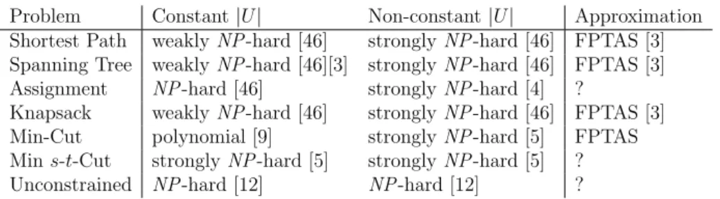
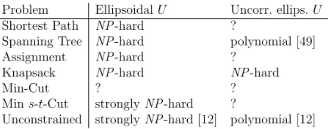
In this thesis we analyze the complexity of the afore mentioned problem for convex and for discrete uncertainty setsU. We will show that under further assumptions the problem is as easy as the underlying combinatorial problem for convex uncertainty sets if the number of calculated solutions is greater than the dimension of the problem. Additionally we present a practical exact algorithm to solve the min-max-min problem for any combinatorial problem, given by a deterministic oracle. On the other hand we prove that if we fix the number of solutions k, then the problem is NP-hard even for polyhedral uncertainty sets and the unconstrained binary problem. For the case when the number of calculated solutions is lower or equal to the dimension we present a heuristic algorithm which is based on the exact algorithm above. Both algorithms are tested and analyzed on random instances of the knapsack problem, the vehicle routing problem and the shortest path problem.
For discrete uncertainty sets we show that the min-max-min problem isNP -hard for a selection of combinatorial problems. Nevertheless we prove that it can be solved in pseudopolynomial time or admits an FPTAS if the min-max problem can be solved in pseudopolynomial or admits an FPTAS respectively.
In dieser Arbeit f¨uhren wir einen Ansatz in der robusten Optimierung ein, der auf einem bin¨aren Min-max-min Problem basiert. Die sogenannte Min-max-min robuste Optimierung erweitert die klassische robuste Optimierung, indemk verschiedene L¨osungen anstatt einer Einzigen berechnet werden. Im Allgemeinen betrachtet man in der robusten Optimierung Probleme, deren Problemparameter unsicher sein k¨onnen. Die Grundidee ist eine Un-sicherheitsmenge U zu definieren, die alle relevanten Problemparameter ent-h¨alt, die man auch Szenarien nennt. Das Ziel ist es eine L¨osung zu berechnen, die f¨ur alle Szenarien in U zul¨assig ist und die den schlechtesten Zielfunk-tionswert bez¨uglich aller Szenarien in U optimiert.
Als Spezialfall desK-adaptability Ansatzes f¨ur zweistufige robuste Probleme, ist es das Ziel des robusten Min-max-min Ansatzesk verschiedene L¨osungen f¨ur das zugrundeliegende kombinatorische Problem zu berechnen, sodass der schlechteste Fall ¨uber alle Szenarien optimiert wird, w¨ahrend wir f¨ur jedes Szenario die beste derk L¨osungen betrachten. Diese Idee kann als Min-max-min Problem modelliert werden.
In dieser Arbeit untersuchen wir die Komplexit¨at des zuvor beschriebenen Problems f¨ur konvexe und f¨ur diskrete Unsicherheitsmengen U. Wir zeigen, dass das Problem f¨ur konvexe Unsicherheitsmengen unter weiteren Voraus-setzungen genau so einfach ist wie das zugrundeliegende kombinatorische Problem, falls die Anzahl der zu berechnenden L¨osungen gr¨oßer als die Di-mension des Problems ist. Desweiteren pr¨asentieren wir einen praktischen ex-akten Algorithmus, der das Min-max-min Problem f¨ur alle kombinatorischen Probleme l¨ost, die durch ein Orakel gegeben sind. Andererseits beweisen wir, dass das Problem f¨ur eine feste Anzahl von L¨osungenNP-schwer ist, sogar f¨ur polyedrische Unsicherheitsmengen und das unrestringierte bin¨are Problem. F¨ur den Fall, dass die Anzahl der L¨osungen kleiner oder gleich der Dimen-sion des Problem ist, pr¨asentieren wir einen heuristischen Algorithmus, der auf dem zuvor erw¨ahnten exakten Algorithmus basiert. Beide Algorithmen wurden an zuf¨alligen Instanzen des Rucksackproblems, des Vehicle-Routing-Problems und des k¨urzesten Wege Problems getestet und analysiert.
F¨ur diskrete Unsicherheitsmengen zeigen wir, dass das Min-max-min Prob-lem NP-schwer ist f¨ur eine Auswahl an kombinatorischen Problemen. Den-noch konnten wir zeigen, dass das Problem in pseudopolynomieller Zeit gel¨ost werden kann bzw. in polynomieller Zeit beliebig genau approximiert werden kann, falls das zugeh¨orige min-max Problem die jeweilige Eigenschaft hat.
Most of the results on convex and discrete uncertainty sets in Chapter 4 and 5 were developed together with my supervisor Christoph Buchheim from TU Dortmund University and can be found in [23, 24].
The computations for the vehicle routing problem in Section 6.1.2 were per-formed in a cooperation with Uwe Clausen and Lars Eufinger from the In-stitute of Transport Logistics at TU Dortmund University.
Acknowledgements
I would like to thank all my colleagues at the University of Dortmund who I met during my time at the university and who worked together with me for at least a small period. Thank you for helping me with my mathematical problems but also for helping me and giving me advice in all other situations in life. Especially I want to thank my supervisor Christoph Buchheim who always supported me and my research work and who always had an open door to answer questions and giving advices.
Furthermore I want to thank my family and all my friends for being always there for me.
1 Introduction 1
2 Preliminaries 5
2.1 Linear Optimization . . . 5
2.1.1 Polyhedra and Cones . . . 6
2.1.2 Duality . . . 10 2.2 Convex Optimization . . . 11 2.2.1 Duality . . . 13 2.3 Complexity Theory . . . 14 2.3.1 Oracles . . . 20 2.4 Combinatorial Optimization . . . 23
2.4.1 The Shortest Path Problem . . . 24
2.4.2 The Minimum Cut Problem . . . 26
2.4.3 The Minimum Spanning Tree Problem . . . 27
2.4.4 The Matching Problem . . . 28
2.4.5 The Knapsack Problem . . . 29
2.4.6 The Unconstrained Binary Problem . . . 29
2.5 Multicriteria Optimization . . . 30
3 Combinatorial Robust Optimization 33 3.1 Strict Robustness . . . 37
3.1.1 Discrete Uncertainty . . . 40
3.1.2 Convex Uncertainty . . . 42
3.5 Adjustable Robustness . . . 52
3.5.1 K-Adaptability . . . 54
3.6 Bulk Robustness . . . 56
4 Min-max-min under Convex Uncertainty 59 4.1 The Case k≥n+ 1 . . . 64 4.1.1 Complexity . . . 65 4.1.2 Exact Algorithm . . . 71 4.2 The Case k < n+ 1 . . . 73 4.2.1 Complexity . . . 73 4.2.2 Heuristic Algorithm . . . 78
5 Min-max-min under Discrete Uncertainty 83 5.1 Complexity . . . 84
5.1.1 Shortest Path Problem . . . 85
5.1.2 Spanning Tree Problem . . . 88
5.1.3 Assignment Problem . . . 90
5.1.4 Minimum Cut Problem . . . 93
5.1.5 Unconstrained Binary Problem . . . 96
5.1.6 Knapsack Problem . . . 98 5.2 Pseudopolynomial Algorithms . . . 99 5.3 Approximation Complexity . . . 101 6 Experiments 105 6.1 Exact Algorithm . . . 106 6.1.1 Knapsack Problem . . . 106
6.1.2 Vehicle Routing Problem . . . 109
6.2 Heuristic Algorithm . . . 118
Introduction
Combinatorial optimization problems occur in many real-world applications e.g. in the industry or in natural sciences and are intensively studied in the optimization literature. A wide range of problems has been solved yet and the algorithms are continuously improved to run faster and to solve larger instances. A famous problem which is often solved e.g. in the logistic industry is thevehicle routing problem. Consider a parcel service which owns a fleet of vehicles and which has to deliver parcels to its customers every day. The vehicle routing problem calculates a tour for each vehicle such that each customer is served by one vehicle and such that on each tour the total demand of the customers does not exceed the capacity of the vehicle. The objective is to find such a set of tours which has minimal cost e.g. minimal travel time. This problem is known to be hard to solve in practice in the sense that an optimal solution can not be calculated in a reasonable time for high-dimensional instances. In this case often approximation algorithms or even heuristic algorithms are used.
In this thesis we study combinatorial problems which can be formulated as min
x∈X c >
x+c0, (M)
where X ⊆ {0,1}n are the incidence vectors of all feasible solutions of the
problem, c ∈ Rn is a cost-vector and c
0 ∈ R a constant. We call (M) the deterministic problem or theunderlying combinatorial problem.
If we want to solve a combinatorial problem in a real-world application we often have to deal with uncertainty in the problem parameters. For example the traveling times of a vehicle can be uncertain because every day a different traffic situation can occur. Depending on the size of the problem, calculat-ing an optimal solution for the vehicle routcalculat-ing problem in the morncalculat-ing after
the traffic scenario is observed, can be inefficient. One approach to tackle uncertainty in the problem parameters is the robust optimization approach. Here for an uncertainty set U which contains all relevant scenarios of the uncertain parameters, the objective is to find a solution which is feasible for every scenario and which optimizes the worst objective value over all scenar-ios. In this thesis we assume that the uncertainty only affects the objective function, i.e. every scenario is given by a cost vector (c, c0) ∈ U ⊆ Rn+1.
Then the robust counterpart of (M) is the problem min
x∈X (c,cmax0)∈U
c>x+c0. (M2)
This problem is known to be NP-hard for several combinatorial problems and several classes of uncertainty sets. Furthermore in practical applications an optimal solution of (M2) is often too conservative in the sense that its objective value can be very bad in many scenarios. Especially in practical applications robust solutions are often not useful.
In the robust optimization literature many different approaches have been presented to find less conservative solutions for problems with uncertain pa-rameters. For example theK-adaptability approach aims to calculateK dif-ferent solutions to approximate a robust two stage problem [41]. Here the variables of the problem are divided into first-stage variables x which have to be calculated before the scenario is known and second-stage variables y which can be calculated afterwards. In this thesis we consider the special case where only one stage exists and propose to solve deterministic problems (M) with uncertain objective functions (c, c0)∈U by adressing the problem
min
x(1),...,x(k)∈X (c,cmax0)∈U i=1min,...,kc >
x(i)+c0 (M3)
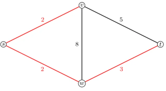
where k ∈ N is a given number of solutions. Clearly the approach is an ex-tension of the min-max approach (M2), which is obtained for k = 1, and yields a better objective value in general. As a motivation consider the par-cel service again. Instead of calculating a solution every morning after the scenario is known, by Problem (M3) a set of k solutions can be calculated once in a perhaps expensive preprocessing. Afterwards each morning when the actual scenario is known the best of the calculated solutions can be easily chosen by comparing the objective values. Furthermore the min-max-min ap-proach (M3) hedges against uncertainty in a robust way and even gives more
flexibility to the user, since he can choose the solution which has most of the properties which he prefers from his personal experience and the solutions do not change over time.
present all necessary definitions and results for linear, multicriteria and con-vex optimization problems and we define all combinatorial problems which we will study in this thesis. Furthermore we give a short introduction to com-plexity theory. In Chapter 3 we will present a selection of robust optimization approaches and discuss the complexity of the related robust counterparts. The main contribution of this thesis is the analysis of the complexity of Problem (M3) for convex uncertainty sets in Chapter 4 and for discrete un-certainty sets in Chapter 5. Additionally to the theoretical results we provide several algorithms to solve Problem (M3) for the specific uncertainty classes
and for several combinatorial problems. Finally in Chapter 6 we present the results of our experiments for the knapsack problem, the shortest path prob-lem and the vehicle routing probprob-lem and give a practical proof that the algorithms presented in Chapter 4 work well on random instances for the afore mentioned problems.
Preliminaries
2.1
Linear Optimization
In this section we will give a short introduction to linear optimization and polyhedral theory. We will quote basic definitions and results which are used in the following chapters. For a detailed description of the results in this section see [45, 40, 54].
We define a linear program as a minimization problem of the form min c>x
s.t. Ax≤b x∈Rn
(P)
where c ∈ Rn, A ∈
Rm×n and b ∈ Rm. Any x ∈ Rn, which fulfills the
constraints, i.e. it is contained in the setP :={x∈Rn | Ax≤b}, is called a feasible solution. Note that by the transformation
min x∈P c > x=−max x∈P −c > x
any linear program of the form (P) can be transformed to an equivalent maximization problem. The main objective in linear programming is to find an optimal solution of problem (P). Here a feasible solutionx∗ ∈P is called
optimal solution if c>x∗ ≤ c>x for all x ∈ P. We then say v := c>x∗ is the optimal value of (P). The function f : P → R with f(x) = c>x is called objective function. If no feasible solution exists, i.e. P is empty, then the problem is called infeasible. The problem is called unbounded if for any α∈Rthere exists anx∈P with c>x < α. We then define the optimal value by−∞.
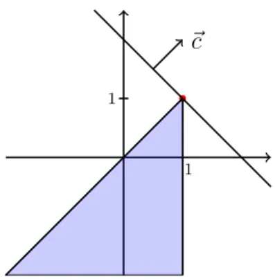
Example 2.1. Consider the linear program max x1+x2 s.t. −x1 +x2 ≤0 x1 ≤1 −x2 ≤2 x1, x2 ∈R (2.1)
which is of the form (P). The unique optimal solution is (x1, x2) = (1,1)
with an optimal value of 2 (see Figure 2.1).
1 1
~c
Figure 2.1: Thefeasible set and theoptimal solution of the Problem (2.1).
In literature many different methods and algorithms have been developed to solve linear optimization problems. In general any linear program can be solved theoretically efficient by the ellipsoid method [40]. But since this method is not very practical to implement it is rarely used to solve problems of the form (P). A practically efficient method to solve general linear prob-lems is thesimplex method which is very fast for many problems in practice and which is easier to implement. Nonetheless in the worst case its theoretical run-time can be exponential [40]. Besides the latter methods many problem-specific algorithms have been developed, which make use of the structure and the properties of (P) for a given problem.
2.1.1
Polyhedra and Cones
We now define two classes of sets, polyhedra and cones, which are of high importance for optimization theory as well as for the framework of robust
optimization. A polyhedron is a set of the form
P ={x∈Rn | Ax≤b} (2.2)
with a matrixA∈Rm×nand a vectorb ∈
Rm. A polyhedron is calledpolytope
if it is bounded, i.e. if there exists a radius R >0 such that P ⊂BR(0) :={x∈Rn | kxk2 ≤R},
where k · k2 is the Euclidean norm. The description (2.2) is called an outer description ofP. For a nonzero vectord∈Rn andδ ∈
R, we call a set of the
form
H :=x∈Rn | d>
x=δ a hyperplane. Furthermore we define
H− :=x∈Rn | d>x≤δ .
AfaceofP is a subsetF ⊆P such that a hyperplaneHexists withF =P∩H andP ⊆H−. A face with a dimension of dim(P)−1 is calledfacet. A face with dimension 0 is calledvertex. The dimension here is defined by the concept of
affine independence. We say the vectorsx0, x1. . . , xkare affinely independent
ifx1−x0, . . . , xk−x0are linearly independent. The dimension of a setS⊆Rn
is then defined by dim(S) := max k∈N∪ {0} | x0, . . . , xk ∈S affinely independent . If the dimension is n, then the set S is called full-dimensional. For such a full-dimensional set S there always exists a point s0 ∈ S and a radius r > 0
such that
Br(s0) :={x∈Rn | kx−s0k2 ≤r} ⊆S.
We callBr(s0) the ball around s0 with radiusr.
A set C ⊆ Rn is called (convex) cone if for any x, y ∈ C and λ, µ ≥ 0 the
point λx+µy is also contained in C. Example 2.2. The set
Rn+ :={x∈R
n | x≥0}
is a cone. Furthermore Rn+ is a polyhedron with exactly one vertex 0 and facets
x∈Rn
+ | xi = 0 for eachi= 1, . . . , n. Note thatRn+is not a polytope
since it is not bounded. An example of a cone which is not a polyhedron is the second-order cone
Kn :=
Both, cones and polyhedra, are convex sets. Here a set U ⊆Rn is convex if
for each x, y ∈ U and 0 ≤ λ ≤ 1 the point λx+ (1−λ)y is also contained inU. We define the convex hull of a set X ⊆Rn as
conv (X) := ( x= k X i=1 λixi | λi ≥0, xi ∈X, k X i=1 λi = 1, k∈N )
and theconic hull of X ⊆Rn as
cone (X) := ( x= k X i=1 λixi | λi ≥0, xi ∈X, k ∈N ) .
The convex hull (conic hull) of X is the smallest convex set (cone) which contains X. The famous Theorem of Carath´eodory states that any point in the convex hull of X ⊆ Rn can be obtained as a convex combination of at
most n+ 1 points in X.
Theorem 2.3 (Theorem of Carath´eodory). For any set X ⊆ Rn and any
point x ∈ conv (X) there exist x1, . . . , xk ∈ X with k ≤ n + 1 such that
x∈conv (x1, . . . , xk).
It is easy to verify that any polytope with vertices x1, . . . , xk is equal to the
set conv (x1, . . . , xk). In particular a setP is a polytope if and only if it is the
convex hull of a finite set of points [45]. For general polyhedra the following theorem holds [54].
Theorem 2.4(Theorem of Weyl-Minkowski). A setP ⊆Rnis a polyhedron
if and only if
P = conv (x1, . . . , xk) + cone (y1, . . . , ym) (2.3)
for x1, . . . , xk, y1, . . . , ym ∈Rn.
The representation (2.3) ofP in the latter theorem is calledinner description
ofP. It is always possible to transform an outer description of a polyhedron into an inner description of the same polyhedron and the other way round. Nevertheless the size of the two descriptions can be different as the following example shows.
Example 2.5. Consider the cube B := [0,1]n ⊂ Rn. Clearly an outer
de-scription of B is given by
B ={x∈Rn | 0≤x i ≤1}
and B can therefore be described by 2n inequalities. On the other hand an inner description of B is given by
B = conv ({0,1}n)
which involves 2n vectors. It is easy to see that no inner description exists
which uses a smaller number of vectors. To show the other direction if we consider the inner description
P := conv ({ei,−ei | i= 1, . . . , n}),
where ei is the i-th unit-vector, then it can be shown that P has an
expo-nential number of facets, and therefore any outer description must have an exponential number of inequalities. But the inner description is given by 2n vectors.
Since the run-time of an algorithm can depend on the size of the description it is important to mention which type of description we use.
A polyhedron P is called rational if any face of P contains a rational point. From the definition it follows directly that any vertex ofP must be rational. Therefore a polytope is rational if and only if it can be described as the convex hull of rational points. Equivalently a rational polytope can be described by an outer description which has only rational entries. We call a polyhedronP
well-described if an outer description P =x∈Rn |a>
i x≤bi, i= 1, . . . , m
exists such that the binary encoding-length of each vector (ai, bi) is bounded
by a value ϕ ∈ Q. We then say P has facet-complexity of at most ϕ. The following lemma shows a relation between the facet complexity and the en-coding size of the vertices of P.
Lemma 2.6 ([40]). If there exists an inner description P = conv (V) + cone (E) such that the binary encoding-length of each vector in V and E is bounded by ν ∈Q, thenP has facet-complexity of at most 3n2ν.
As a corollary we obtain that if each vertex of a polytope P has encoding-length of polynomial size, thenP has facet-complexity of polynomial size. Example 2.7. Consider the polytopeP := conv (X) withX ⊆ {0,1}n. Since
the binary encoding length of each vertex in X is bounded by n it follows from Lemma 2.6 that P has facet-complexity of at most 3n3. Therefore P is
well-described and an outer description ofP exists such that each inequality has encoding length of at most 3n3.
Note that the definition of the facet-complexity above does not take into account the number of inequalities m in the outer description. Hence if each outer description of a polyhedron has an exponential number of inequalities, it can still have a polynomial facet-complexity. We will go into detail about this topic in Section 2.3.
2.1.2
Duality
Duality is an important concept which is applied to linear optimization prob-lems but also to general optimization probprob-lems. For a given minimization problem, theprimal problem, the basic idea is to find a related, so calleddual problem, which computes the best lower bound on the optimal value of the primal problem. Depending on the class of optimization problems one can give conditions under which the optimal values of the dual and the primal problem coincide. Thedual problem of (P) is given by
max −b>y s.t. A>y =−c
y≥0.
(D)
In Section 2.2 we show how the dual problem can be derived for general convex optimization problems and, as a special case, how (D) can be derived for linear problems. Clearly for any feasible solutionxof (P) and any feasible solutiony of (D) it holds
y>b≤y>Ax=c>x
since y ≥ 0 and y and x are feasible. Therefore the optimal value of the dual problem gives always a lower bound on the optimal value of the primal problem. In fact both optimal values are equal if both problems have feasible solutions.
Theorem 2.8 ([45]).
(i) If (P) and (D) are both feasible, then their optimal values are the same. (ii) If (P) has an optimal solution then (D) has an optimal solution and
both optimal values are the same.
Example 2.9. The dual problem of the problem in Example 2.1 is min y2+ 2y3
s.t. −y1+y2 = 1
y1−y3 = 1
y1, y2, y3 ≥0
with the optimal solution (1,2,0) and an optimal value of 2.
2.2
Convex Optimization
In this section we will give a short introduction to problems and tools of the theory of convex optimization. For a detailed description of the topic see [22]. A generalconvex optimization problem is a problem of the form
min f0(x)
s.t. fi(x)≤0, i= 1, . . . , m
Ax=b x∈Rn
(COP)
where the functions f0, . . . , fm :Rn →R are convex, i.e. they satisfy
fi(γx+ (1−γ)y)≤γfi(x) + (1−γ)fi(y)
for all x, y ∈ Rn and all γ ∈ [0,1]. Here A ∈
Rp×n and b ∈ Rp. There
are many sub-classes of convex problems which can be solved by special methods and algorithms e.g. linear programs. Another sub-class are the so called quadratically constrained quadratic problems which are of the form
min x>P0x+q0>x+r0
s.t. x>Pix+qi>x+ri ≤0, i= 1, . . . , m
Ax=b x∈Rn
(QCQP)
where each Pi is a symmetric positive semidefinite n ×n matrix, qi ∈ Rn,
ri ∈ R and A, b are defined like above. Note that because all Pi are positive
semidefinite the functions
fi(x) :=x>Pix+q>i x+ri
Example 2.10. LetE =
x∈Rn |(x−x)¯ >Σ(x−x)¯ ≤Ω2 be an ellipsoid
with center-point ¯x ∈ Rn, positive definite matrix Σ ∈
Rn×n and Ω ∈ R.
Then optimizing a linear function over the ellipsoid U can be modeled as a (QCQP) by
max c>x
s.t. x>Σx−(2Σ¯x)>x+ ¯x>Σ¯x−Ω2 ≤0 x∈Rn.
It was shown in [40], that ¯
x>c+ Ω√c>Σ−1c
is the optimal value of the latter problem (see Figure 2.2).
¯ x c Σ−1c √ c>Σ−1c ¯ x+√Σ−1c c>Σ−1c
Figure 2.2: Maximization ofc>xoverE =x∈Rn | (x−x)¯ >Σ(x−x)¯ ≤1 .
A more general problem than (QCQP) is thesecond-order cone problem
min c>0x
s.t. kPix+qik2 ≤c>i x+di, i= 1, . . . , m
Ax=b x∈Rn
(SOCP)
where Pi ∈Rni×n, qi ∈ Rni, ci ∈Rn, di ∈ R and A, b are defined like above.
Note that each of the first m constraints describes a second-order cone in dimension ni+ 1. Since for any positive semidefinite matrixP there exists a
matrixB such thatP =B>B, we can transform any quadratic constraint of the formx>P x+q>x+r≤0 into the equivalent second-order cone constraint
B 1 2q > x+ 0 1 2(1 +r) 2 ≤ 1 2 1−q > x−r .
Hence (QCQP) is a special case of (SOCP). In general Problem (SOCP) and therefore Problem (QCQP) can be solved in polynomial time by the interior-point method up to an arbitrary accuracy [8].
2.2.1
Duality
In this section we will give an instruction how to dualize convex problems and we will give a condition under which strong duality holds. For the convex problem (COP) the Lagrange dual function L:Rm+ ×Rp →
R is defined by L(λ, ν) = inf x∈Rn f0(x) + m X i=1 λifi(x) + p X i=1 νi(a>i x−bi) !
where ai is the i-th row of A.
Lemma 2.11 ([22]). Let p∗ be the optimal value of problem (COP). Then for any λ∈Rm
+ and ν ∈Rp the inequality
L(λ, ν)≤p∗ is valid.
Hence the Lagrange dual function gives a lower bound on the optimal value of Problem (COP) for any λ ∈ Rm
+ and ν ∈ Rp. Now a natural question is:
what is the best of these lower bounds? The answer is the optimal value of the so calledLagrange dual problem
max L(λ, ν) s.t. λ ∈Rm
+
ν ∈Rp.
(2.4)
In the following letd∗be the optimal value of (2.4). From Lemma 2.11 follows d∗ ≤ p∗. The following theorem gives a sufficient condition, called Slater’s Condition, under whichstrong duality holds, i.e. d∗ =p∗.
Theorem 2.12 ([22]). If there exists a vector x ∈ Rn such that f
i(x) < 0
for all i= 1, . . . , mand Ax=b then d∗ =p∗ holds.
In fact a weaker version of Slater’s condition can be proved. To obtain strong duality it suffices if there exists a point x ∈ Rn such that strict inequality
fi(x)<0 holds for all non-affine functionsfi while for the affine functions fj
In the following example we derive the dual problem (D) presented in Sec-tion 2.1.2 for linear optimizaSec-tion problems. The idea of the following calcu-lations will also be used in Section 4.1 to transform problem (M3).
Example 2.13. The Lagrange dual function of the primal problem (P) is given by L(λ) = inf x∈Rn c>x+λ>(Ax−b) =−λ>b+ inf x∈Rn c > +λ>Ax = ( −λ>b, c>+λ>A= 0 −∞ otherwise for all λ≥0. Therefore the Lagrange dual problem is
max −λ>b s.t. c> =−λ>A
λ≥0
which is exactly problem (D). Note that either (P) has no feasible solution or we can apply the weaker version of Slater’s condition and obtain strong duality which was already given in Theorem 2.8.
Finally we will state a famous result from convex analysis called minimax theorem, which allows us to dualize min-max problems.
Theorem 2.14([51]). LetX ⊆RnandY ⊆
Rmbe non-empty closed convex
sets and let f :X×Y →R be a continuous function which is concave in X for everyy ∈Y and convex inY for everyx∈X. If eitherXorY is bounded then
inf
y∈Y supx∈Xf(x, y) = supx∈Xyinf∈Y f(x, y).
2.3
Complexity Theory
In this thesis our main objective is to analyze the complexity of problem (M3). Hence in this section we give a short introduction to complexity theory and present results which we use in the following chapters. To get a precise and detailed description of this topic see [45].
In complexity theory the aim is to analyze how difficult it is to solve a problem. On the one hand if an algorithm to solve a problem is known, we
are interested in upper bounds on the worst-case run-time of the algorithm to get an idea how fast the algorithm is. On the other hand we want to classify problems by their difficulty. If a problem A can be used to solve a different problem B without doing additional expensive calculations, then we can say that Problem B is not harder than Problem A, since we can always solve it by solving Problem A.
In this thesis analgorithm is defined for a set of validinputs and is a sequence of instructions which calculate for any input a certain output in a finite number of steps. A step in an algorithm can be arithmetic operations like addition, subtraction, multiplication, division and comparison of numbers, but also variable assignments. For an exact definition of this see the definition of Turing machines in [45].
In the following let L:={0,1}∗ be the set of all finite strings of 0’s and 1’s.
Any subset of L is called language. We will use L to describe all necessary objects of our problems. For any x ∈ L we define the size of x, denoted by hxi, as the number of 0’s and 1’s in x. For the description of numerical values we assume the binary encoding scheme in this thesis, i.e. every value is described by its binary stringv ∈L. We sayf :N→Nis arun-time function
for an algorithm A if for any input i∈ L of sizen, the algorithm calculates an output in at most f(n) steps. The algorithm is called polynomial-time algorithm (or has polynomial run-time) if a run-time function f exists such that f(n) ≤ p(n) for all n ∈ N for some polynomial p. An algorithm has
constant run-time if f(n)≤c for all n ∈N and a constant c∈ N. We often write O(f) to denote the run-time of an algorithm.
Given a languageI ⊆ {0,1}∗, a functionf :I → {0,1}∗ and an algorithm A
which calculates for any i∈I the ouput f(i)∈ {0,1}∗, then we say A com-putesf. If for a givenf a polynomial time algorithm exists which computesf then we sayf iscomputable in polynomial time. Iff :{0,1}∗ → {0,1}and A
computes f then we say A decides the language L0 :={l ∈ {0,1}∗ |f(l) = 1}.
If a polynomial time algorithm exists which decides a language L0 then we say L0 is decidable in polynomial time.
We define anoptimization problem as a quadruple Π = (I,(Si)i∈I,(ci)i∈I,goal)
where
• I ⊆ {0,1}∗ is a language decidable in polynomial time;
• Si ⊆ {0,1}∗ is nonempty for each i ∈ I and a polynomial p exists
with hyi ≤ p(hii) for all i ∈ I and y ∈ Si; furthermore the language {(i, y)| i∈I, y∈Si} is decidable in polynomial time;
• ci :Si →Qfor eachi∈I is a function computable in polynomial time;
• goal∈ {max,min}.
The elements of I are called instances. For each instance i ∈ I we call Si
the set of feasible solutions and ci the objective function of i. Note that by
the assumptions given in the listing above we make sure that an algorithm exists which can decide in polynomial time if a given string i ∈ {0,1}∗ is a
valid instance of the problem and for any y ∈ Si if y is a feasible solution.
Furthermore we assume that we can calculate the objective value for each feasible solution in polynomial time.
An (exact) algorithm A for Π is an algorithm which computes for each in-stancei∈I a feasible solution y ∈Si such that
ci(y) = goal{ci(y0) :y0 ∈Si}.
The computed solution is called optimal solution and its objective function value ci(y) is denoted by opt(i). We define the size of an instance i of an
optimization problem byhii =hSii+hcii+ 1. The size of the latter objects
depends on the description of the object which is used. As we have seen in Example 2.5 the size of a description of the same object can vary a lot. Example 2.15. For an inner description
P = conv (x1, . . . , xm) + cone (e1, . . . , el) the size ofP is hPi= m X i=1 hxii+ l X i=1 heii.
If P is given by an outer description P = {x∈Rn | Ax≤b} then the size
of P is hPi= m X i=1 h(ai, bi)i.
As we have seen in Section 2.2 the feasible set can be an ellipsoid given by E =x∈Rn | (x−x)¯ >
Σ(x−x)¯ ≤Ω2 . Then the size of E is
hEi=hΣi+hx¯i+hΩi.
If a feasible set U is given by a list of vectors U ={c1, . . . , cm}then the size
ofU ishUi=Pm
i=1hcii. The latter classes of sets of feasible solutions will be
We say f : N → N is a run-time function for an optimization problem Π if for any instance i of size n, an algorithm for Π exists which calculates an optimal solution of instance i in at most f(n) steps. Note that in general the actual run-time for an instance of sizen must not depend exactly on the parameternbut can depend on a much smaller parameter which is part of the instance description. For example as we will see later, certain problems over a polyhedron P = {x∈Rn | Ax≤b} can be solved in polynomial time in
the maximum ofh(ai, bi)iover all row-vectors (ai, bi). Therefore in contrast to
the size ofP the run-time of the algorithm does not depend on the number of rows inA. Note that the run-time of an algorithm can depend on additional parameters given in the input which are not part of the instance description, e.g. an accuracy parameterε >0 for the computations. In this case we have to mention that the run-time function is given in the size of the instance and the respective additional parameters.
The basic classes P and N P are originally defined for so called decision problems. A decision problem is a pair Π = (I, Y), where I ⊆ {0,1}∗ is a
language decidable in polynomial time, called instances, and Y ⊆I are the so-called yes-instances. An algorithm solves Π if it decides for any instance i∈I, if i∈Y or ifi∈I\Y, i.e. the algorithm computes the function
f :I → {0,1}
with f(i) = 1 if i∈ Y and f(i) = 0 otherwise. A detailed description of the following results and an extensive list of decision and optimization problems can be found in [37].
Definition 2.16. The class of all decision problems which can be solved by a polynomial-time algorithm is denoted by P.
Definition 2.17. A decision problem Π = (I, Y) belongs to the class N P if there is a polynomial p and a decision problem Π0 = (I0, Y0) in P where I0 :={ic:i∈I, c∈ {0,1}bp(hii)c}, such that
Y ={y∈I :∃ c∈ {0,1}bp(hii)c:yc∈Y0}. Herec is called a certificate for y.
In other words a problem is inNPif for any yes-instance ythere exists a cer-tificate of polynomial size, with the help of which we can decide in polynomial time that y is a yes-instance.
Example 2.18. The subset-sum problem is defined as follows: An instance is given by integers c1, . . . , cn ∈ Z and K ∈ Z and an instance is a
yes-instance if there exists a set S ⊆ {1, . . . , n} such that P
choose Π0 in the latter definition as the subset-sum problem as well then for each yes-instance the setS is a certificate and by calculatingP
j∈Scj we can
decide in polynomial time if the given instance is a yes-instance. Therefore the subset-sum problem is inNP.
It is easy to prove that P ⊆ N P by choosing p ≡ 0 and Π0 = Π in Defini-tion 2.17. On the other hand the quesDefini-tion if P = N P or not, is one of the most important open problems in complexity theory.
Since we will only work with optimization problems in this thesis we will omit further definitions which are only related to decision problems. Substantial results again can be found in [45].
Definition 2.19. A problem Π1 polynomially reduces to an optimization
problem Π2 = (I,(Si)i∈I,(ci)i∈I,goal) if for a given function f defined by
f(i) = {y∈Si :ci(y) =opt(i)},
there exists a polynomial-time algorithm to solve Π1 using f, where
calcu-latingf(i) for any iis assumed to consume constant run-time.
In other words, if we have an oracle which solves problem Π2 in constant
time, then we can solve problem Π1 in polynomial time. A consequence of
the latter definition is that, if we have a polynomial-time algorithm for Π2,
then we can solve Π1in polynomial time. On the other hand if we would know
that Π1 can not be solved in polynomial-time then Π2 can not be solved in
polynomial time since this would lead to a contradiction. It is easy to see that the latter construction is transitive i.e. if Π1 polynomially reduces to Π2
and Π2 polynomially reduces to Π3 then Π1 polynomially reduces to Π3.
Definition 2.20. An optimization problem Π is called NP-hard if all prob-lems inNP polynomially reduce to Π.
The latter definition implies that the class ofNP-hard problems contains the optimization problems which are at least as hard as the hardest problems in NP. To show that a problem Π is NP-hard, by the transitivity of the reduction, it suffices to reduce anyNP-hard problem to Π.
Proposition 2.21. If an NP-hard problem Π1 polynomially reduces to an
optimization problem Π2 then Π2 isNP-hard.
Ifi consists of a list of integers then in the following we denote by largest(i) the largest of these integers.
Definition 2.22. Let Π be an optimization problem such that each instancei consists of a list of integers. An algorithm for Π is called pseudopolynomial
if its run-time is bounded by a polynomial inhii and largest(i). AnNP-hard optimization problem for which a pseudopolynomial algorithm exists is called
weakly NP-hard.
In other words the run-time of a pseudopolynomial algorithm depends on the values of the numbers ini. It can have exponential run-time in its worst-case even if all numbers can be encoded in polynomial size. But if the value of all occurring numbers has polynomial size, the algorithm is a polynomial-time algorithm.
Example 2.23. The knapsack problem, which we will define properly in Section 2.4, is known to be NP-hard (see Theorem 2.46). Nevertheless there exists a dynamic programming algorithm to solve the problem (see [44]) which has run-time O(nb) where b is the knapsack capacity. Clearly this is a pseudopolynomial algorithm. Note that if we choose b = 2n then the size
of b is linear in n, since we assume binary encoding, but the run-time of the algorithm is n2n in its worst-case which is exponential in the size of b.
Problems which can not have a pseudopolynomial algorithm, unlessP =N P, are the following:
Definition 2.24. Let Π be an optimization problem such that each instance consists of a list of integers and for any polynomial p let Πp be the same
problem restricted to only the instancesi∈I with largest(i)≤p(hii). Prob-lem Π is called strongly NP-hard if there is a polynomial p such that Πp is NP-hard.
Lemma 2.25. Let Π1 and Π2 be optimization problems. If Π1 is strongly NP-hard and polynomially reduces to the problem (Π2)p for a polynomial p,
then Π2 is strongly NP-hard.
In other words the latter lemma states that if all the numbers used by the reduction algorithm have polynomial size then reducing a strongly NP-hard problem yields strongly NP-hardness. For problems which are hard to solve, sometimes also non-optimal solutions are accepted by a user if we can give a certain guarantee for the quality of the solution.
Definition 2.26. Let Π be an optimization problem with a non-negative optimal value and ε >0. An algorithmA is an ε-approximation algorithm if for any instancei of Π it calculates a feasible solution y∈Si with
1
Problem Π has afully polynomial approximation scheme if for anyε >0 there exists anε-approximation algorithm whose run-time as well as the maximum size of any number occurring in the computation is bounded by a polynomial inhii+hεi+1
ε. We then say that Π admits an FPTAS.
2.3.1
Oracles
In Section 4.1.1 we will give an oracle-based algorithm which uses several results from [40]. Therefore we will give a short introduction to the results which we use later. For a detailed description see [40].
We define anoracle as an algorithmOwith constant run-time which returns, for an input σ ∈ {0,1}∗ of size n, an output of size at most p(n) for a
polynomialp. We can consider an oracle as a procedure which gives an answer to a question or a solution for a problem without increasing the run-time except by a constant number of steps. An oracle-polynomial algorithm A is an polynomial-time algorithm which uses O. We also say A runs in oracle-polynomial time. In Section 4.1.1 we will use oracles for optimization and separation problems. The latter problems are defined as follows for convex and compact setsK ⊆Rn:
Problem 2.27(The Strong Optimization Problem). Given a vectorc∈Rn,
find a vectory∈K that maximizes c>x overK or assert that K is empty. Problem 2.28 (The Strong Separation Problem). Given a vector y ∈ Rn,
decide whether y ∈K, and if this is not the case, find a vector c∈Rn such
that c>y >max{c>x| x∈K} holds.
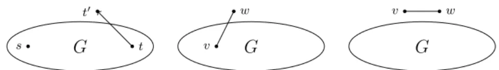
In fact the latter problem is to find a so-called cutting-plane, i.e. a hyper-planeH which cuts off the pointy if it is not contained inK. More precisely we want to find a hyperplane H such that K ⊆H− but y /∈ H− if it is not contained in K.
y c
H
K
Based on the latter two problems a very famous result from [40] can be cited, which states that optimization and separation are polynomially equivalent. In the following for a well-described polyhedronP ⊆Rnwe define thefacet-size
ofP byhPiF =n+ϕ, whereϕis the facet-complexity ofP. This is motivated
by the fact that the algorithms in [40] iteratively call the separation oracle or the optimization oracle respectively a polynomial number of times no matter how many inequalities are given in the description of P. The computations only depend on an upper bound on the size of each inequality on its own. Theorem 2.29 ([40]). Given an oracle for the strong separation (optimiza-tion) problem, the strong optimization (separa(optimiza-tion) problem can be solved in oracle-polynomial time inhPiF for any well-described polyhedron P.
Example 2.30. As we have seen in Example 2.7 the facet-complexity of P := conv (X) with X ⊆ {0,1}n is at most 3n3. An optimization oracle for
the deterministic problem
min
x∈Xc >x
yields an optimization oracle for the equivalent problem min
x∈P c >
x
and hence from Theorem 2.29 follows that we can solve the separation prob-lem over P in time polynomial in 3n3+n.
Given an optimization oracle it is possible to calculate a convex combination for any rational point in a well-described polyhedron in polynomial time. Theorem 2.31([40]).For any well-described polyhedronP given by a strong optimization oracle and for any rational vectory0 ∈P, there exists an
oracle-polynomial time algorithm in hPiF +hy0i, that finds affinely independent
vertices x0, . . . , xk of P and rational λ0, . . . , λk ≥ 0 with
Pk
i=0λi = 1 such
that y0 =
Pk
i=0λixi.
Note that since the vertices calculated by the latter algorithm are affinely in-dependent the algorithm calculates at mostn+1 vertices. The latter theorem especially states that for each rational point x∗ ∈conv (X) we can calculate a convex combination of points in X for x∗ in polynomial time if we can linearly optimize over conv (X) in polynomial time, which is equivalent to linear optimization over X.
For general convex problems the equivalence in Theorem 2.29 is not true. If we are considering arbitrary convex sets K, we even have to take into account
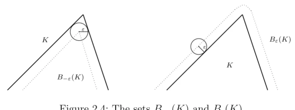
irrational values, which can occur for example if we consider expressions involving a norm. Therefore we need a parameter ε > 0 which determines the accuracy of calculations. We define
Bε(K) :={x∈Rn | kx−yk2 ≤ε for some y∈K}
and
B−ε(K) := {x∈K | Bε(x)⊆K}.
By definition Bε(K) contains all points which have a distance to K of at
mostε. The setB−ε(K) contains all points which have a distance of at leastε
to the boundary ofK(see Figure 2.4). It always holdsB−ε(K)⊂K ⊂Bε(K).
Note that ifK is not full-dimensional then B−ε(K) =∅.
ε B−ε(K) K ε K Bε(K)
Figure 2.4: The sets B−ε(K) and Bε(K)
Using the latter definitions we define the weak version of the so called mem-bership problem.
Problem 2.32 (The Weak Membership Problem). Given a vector y ∈ Qn
and any rational value ε >0, assert thaty∈Bε(K) or that y /∈B−ε(K).
Note that both conditions, y ∈ Bε(K) and y /∈ B−ε(K) can be true at the
same time. If we can solve the strong separation problem it directly follows that we can solve the weak membership problem.
In the following a full-dimensional compact convex setK is called a centered convex body if the following information is explicitly given: the integer n such that K ⊆Rn, a positive rational number R such that K ⊆ B
R(0) and
a rational number r and a vector a0 ∈ Qn such that Br(a0) ⊆ K. We then
write K(n, R, r, a0) and the size of K is
hKi:=hni+hεi+hRi+hri+ha0i .
As mentioned before the equivalence of the strong optimization problem and the strong separation problem is not true if we consider convex problems. But,
as the following theorem states, if we consider convex objective functions, given by an oracle and defined over a centered convex body, then solving the weak membership problem in polynomial time yields a polynomial-time optimization-algorithm in a weak version. More precisely:
Theorem 2.33 ([40]). Let ε > 0 be a rational number, K(n, R, r, a0) a
centered convex body given by a weak membership oracle and f :Rn →
R a
convex function given by an oracle which returns for everyx∈Qnand δ >0
a rational number t such that |f(x)−t| ≤ δ. Then there exists a oracle-polynomial time algorithm in hKi and hδi, that returns a vector y ∈Bε(K)
such that f(y)≤f(x) +ε for all x∈B−ε(K).
In other words the theorem states that we can find a vector almost inKwhich almost maximizes the objective function over all vectors which are deep inK. In Section 4.1.1 the latter theorem will be combined with a rounding proce-dure. The idea is to round the pointywhich is calculated in Theorem 2.33 to a denominator such that it is guaranteed to be contained inK. Under certain assumptions, this can also be done in polynomial time, which is shown by the following lemma.
Lemma 2.34 ([40]). Let P ⊆ Rn be a polyhedron such that for ϕ ∈
N
we have hPiF ≤ ϕ and let v ∈ B2−6nϕ(P). Then we can calculate q ∈ Z
with 0 < q < 24nϕ and a vector w ∈
Zn in polynomial time in hϕi and hvi
such that
kqv−wk<2−3ϕ and such that 1qw is contained inP.
2.4
Combinatorial Optimization
In this section we will define the combinatorial optimization problems which will appear in this thesis. While our results in Section 4 hold for any com-binatorial problem which can be described through a set X ⊆ {0,1}n, the
complexity results in Chapter 5 are proved for the combinatorial problems de-fined in this section. We will not give explicit polyhedral formulations for the feasible sets X ⊆ {0,1}n of these problems. This is due to the fact that our
results in Section 4.1.1 can be applied to an arbitrary optimization routine for the underlying combinatorial problem and therefore we do not need any specific formulation of the feasible setX. A detailed analysis of the following results can be found in [45, 54].
Most of the combinatorial problems we are considering are defined on graphs. An undirected graph G = (V, E) consists of a finite set of nodes V =
{v1, . . . , vm} and a finite set of edges E ={e1, . . . , en}. An edge e = {v, w}
is a set of two nodes v, w∈V. In adirected graph, each edge has a direction i.e. it has ahead v and atail w. In this case we writee= (v, w) as a 2-tuple to clarify that the order of the nodes has to be considered. An undirected graph can be easily transformed into a directed graph by replacing each edge e={v, w} by two directed edges e1 = (v, w) and e2 = (w, v). An undirected
graph is called complete if for any two nodes v, w ∈ V there exists an edge
{v, w} ∈E or in the directed case if both edges (v, w) and (w, v) exist. Two edges are called parallel if they are defined for the same pair of nodes and, in the directed case, have the same direction. In this thesis we are consid-ering only simple graphs i.e. graphs without parallel edges. Furthermore we assume that no edges of the form (v, v) exist. Two edges are calledadjacent
if they have a common node. An undirected graph is called bipartite if V can be partitioned in two disjunctive setsV1 and V2 such that for each edge
{v, w} ∈ E holds v ∈ V1 and w ∈ V2. For any subset of edges X ⊆ E we
define the incidence vector 1X :E → {0,1} of X by
1X(e) =
(
1 e ∈X 0 e /∈X.
2.4.1
The Shortest Path Problem
LetG= (V, E) be a directed graph, c:E →R a cost function on the edges of Gand s, t∈V two nodes. A path from s tot is a sequence of edges
pst := (e1, e2, . . . , el)
where the head of e1 is s, the tail of el is t and the tail of ej is equal to the
head of ej+1 for each j = 1, . . . , l−1 while any node in V is traversed at
most once. The cost of path pst is defined by
c(pst) := l
X
j=1
c(ej).
A graph is called connected if for any pair of vertices s, t∈V a path from s to t exists. A cycle C in G is a sequence of edges (pst,(t, s)) for a path pst.
A graph is conservative if each cycle has non-negative cost. The latter defi-nitions can be applied analogously to undirected graphs. The shortest path problem is defined as follows:
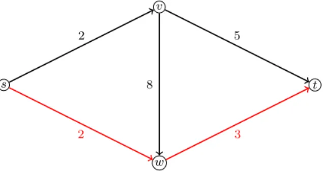
Problem 2.35(Shortest Path Problem). Given a conservative directed graphG together with a cost function c : E → R and two vertices s, t ∈ V, find a path froms to t with minimal cost or decide that no such path exists.
s t v w 2 5 2 3 8
Figure 2.5: Theshortest path with cost 5
The set of all paths in G can be described by a binary set XSP ⊆ {0,1}E
which contains all incidence vectors of paths in G:
XSP ={1P | P ⊆E is a path froms to t in G}.
The following theorem gives two important complexity results on the shortest path problem.
Theorem 2.36 ([54]). The shortest-path problem on conservative graphs can be solved in polynomial time while for arbitrary cost functions it isNP -hard.
Proof. Statement (i) can be verified among others by the by the Moore-Bellmann-Ford Algorithm which has polynomial run-time. For further algo-rithms see [54].
The second statement is proved by reducing the Hamiltonian path problem to the shortest path problem. Given a directed graph G = (V, E) and s, t ∈
V, the Hamiltonian path problem gives an answer to the question if there exists a path from s to t in G which traverses each node in V exactly once. The Hamiltonian path problem is known to be NP-complete [54]. Define the shortest path problem onG by defining cost c(e) =−1 on each edgee ∈E. The shortest path then has cost |V| −1 if and only if a Hamiltonian path exists in G.
2.4.2
The Minimum Cut Problem
LetG= (V, E) be an undirected and connected graph and c:E →R a cost function on the edges of G. A cut in G is a set of edges of the form
δ(S) :=
{v, w} ∈E v ∈S, w ∈V \S
.
for any nonempty set of nodes S ( V. For s, t ∈ V an s-t-cut in G is a cut δ(S) wheres∈S and t ∈V \S. The cost of a cut are defined by
c(δ(S)) := X
e∈δ(S)
c(e).
Problem 2.37 (Minimum Cut Problem). Given an undirected and con-nected graphG= (V, E) and a cost functionc:E →R, find a cut inGwith minimal cost.
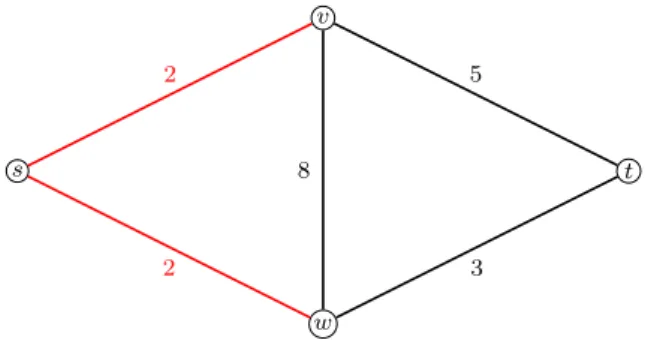
Problem 2.38 (Minimum s-t-Cut Problem). Given an undirected and con-nected graph G= (V, E), two nodes s, t ∈V and a cost functionc:E →R, find as-t-cut in Gwith minimal cost.
s t v w 2 5 2 3 8
Figure 2.6: Theminimum s-t cut with cost 4
The set of all cuts inGcan be described by a binary setXC ⊆ {0,1}E which
contains all incidence vectors of cuts inG:
XC ={1δ(S) | ∅ 6=S (V}.
Theorem 2.39. The minimum cut problem and the minimum s-t-cut prob-lem can be solved in polynomial time.
Proof. By the famous Max-Flow-Min-Cut-Theorem the minimum s-t-cut problem can be solved by the maximum flow problem in polynomial time [54]. On the other hand the minimum cut problem can be solved by calculating the minimum s-t-cut for each pair of nodes s, t ∈ V and return the cut with minimum cost over all pairs. Note that the number of pairs of nodes is
1
2|V|(|V| −1) and is therefore polynomial in the input.
2.4.3
The Minimum Spanning Tree Problem
Let G = (V, E) be an undirected graph and c : E → R a cost function on the edges ofG. Aspanning tree inGis a sub-graphT = (V, E0) with E0 ⊆E such that T contains no cycles and is connected. The cost of a spanning-tree is defined byc(T) :=P
e∈E0c(e).
Problem 2.40(Minimum Spanning Tree Problem). Given a connected undi-rected graph G= (V, E) and a cost functionc:E →R, find a spanning tree inG with minimal cost.
s t v w 2 5 2 3 8
Figure 2.7: Theminimum spanning-tree with cost 7
The set of all possible spanning trees in G can be described by a binary set XST ⊆ {0,1}E which contains all incidence vectors of spanning trees in G:
XST ={1E0 |T = (V, E0) is a spanning tree in G}.
Theorem 2.41 ([45]). The spanning-tree problem can be solved in polyno-mial time.
Proof. The spanning-tree problem can be solved e.g. by the famous algorithm of Kruskal which has polynomial run-time.
2.4.4
The Matching Problem
Let G = (V, E) be an undirected graph and w : E → R a weight function on the edges of G. A matching in G is a set of pairwise non-adjacent edges M ⊆ E. A perfect matching in G is a matching Mp ⊆ E such that for each
nodei ∈V there exists an edge e∈Mp with i∈e. A perfect matching in a
bipartite graph is called assignment. The weight of a matching is defined by w(M) := P
e∈Mw(e). In literature different variants of the matching problem
are studied [45]. In this thesis we will consider the following two variants. Problem 2.42 (Minimum Weight Perfect Matching Problem). Given an undirected graphGand a weight functionw:E →R, find a perfect matching M with minimum weight or decide that Ghas no perfect matching.
Problem 2.43 (Assignment Problem). Given a bipartite graph G, find a perfect matching Mp in G with minimum weight or decide that G has no
perfect matching. s t v w 2 5 2 3 8
Figure 2.8: Theminimum perfect matching with cost 5
The set of all perfect matchings inGcan be described by a binary set XM ⊆ {0,1}E which contains all incidence vectors of perfect matchings inG.
XM ={1M |M ⊆E is a matching inG}.
Theorem 2.44 ([45]). The minimum weight perfect matching problem and the assignment problem can be solved in polynomial time.
Proof. The minimum weight perfect matching problem can be solved in poly-nomial time by the famous algorithm of Edmonds [45]. The assignment prob-lem is a special case of the minimum weight perfect matching probprob-lem which proves the result.
2.4.5
The Knapsack Problem
The Knapsack Problem is defined as follows:Problem 2.45 (Knapsack Problem). Given profits c1, . . . , cn ∈ N, weights
a1, . . . , an ∈ N and a capacity b, find a subset S ⊆ {1, . . . , n} such that
P
j∈Saj ≤b and
P
j∈Scj is maximal.
The set of all feasible subsets S can be described by a binary set XKP ⊆ {0,1}n, which contains all incidence vectors of feasible subsetsS ⊆ {1, . . . , n}:
XKP ={1S | S⊆ {1, . . . , n}:
X
j∈S
aj ≤b}.
Theorem 2.46 ([45]). The Knapsack Problem is weaklyNP-hard.
Proof. To prove that Problem 2.45 is NP-hard we reduce the subset-sum problem to the knapsack problem. For given c1, . . . , cn ∈ Z and K ∈ Z
the subset-sum problem asks if there exists a set S ⊆ {1, . . . , n} such that
P
j∈Scj = K. Define an instance of the knapsack problem by choosing
c1, . . . , cn as profits and setting aj = cj and b = K. Then the knapsack
problem has optimal value K if and only if the answer to the subset sum problem is yes.
A pseudopolynomial algorithm for the knapsack problem which has a run-time ofO(nb) is given by a dynamic programming approach and can be found in [44].
2.4.6
The Unconstrained Binary Problem
In this subsection we introduce the unconstrained binary problem. As we will see the deterministic version of this problem can be solved trivially. But since the robust version (M2) of the problem is NP-hard as we will see later
we will proof complexity results for the min-max-min version as well. The unconstrained binary problem is defined as follows.
Problem 2.47 (Unconstrained Binary Problem). Given profits c1, . . . , cn ∈
Q find a subsetS ⊆ {1, . . . , n}such that Pj∈Scj is minimal.
Since all subsets S ⊆ {1, . . . , n} are feasible, the set of feasible incidence vectors is
Theorem 2.48. The binary unconstrained problem can be solved in linear time.
Proof. Clearly an optimal solution of the binary unconstrained problem is S ={i∈ {1, . . . , n} |ci <0}
which proves the result.
2.5
Multicriteria Optimization
In Section 3.1.1 we derive a relation between robust optimization and multi-criteria optimization which we will extend for Problem (M3) in Section 5.1.
Therefore we give a short introduction to multicriteria optimization in this section. Detailed results about this topic can be found in [30, 31].
We define alinear multicriteria optimization problem by min x∈X c > 1x, . . . , c > mx (2.5) where ci ∈ Rn. Since in this thesis we are interested in combinatorial
opti-mization problems we assume X ⊆ {0,1}n. Obviously in general there does
not exist a point which minimizes all objective functionsci at the same time.
So the main objective in multicriteria optimization is to find efficient solu-tions i.e. solutions for which no other solution exists which is better in every criteria ci. Formally a solution x ∈ X is called efficient if no other solution
y∈ X exists, such that c>i y ≤c>i x for all i= 1. . . , m and c>j y < c>j x for at least one objective functioncj. If such a y exists, then x is calleddominated
byy. One objective in multicriteria optimization can be to find the set of all efficient solutions XE. Note that for X ⊆ {0,1}n the set XE can have
expo-nential size, as it was shown for several combinatorial problems [31]. There are several different methods to find efficient solutions for multicriteria prob-lems. A well-studied method is the weighted-sum method [30]. Here the idea is to solve the deterministic problem
min x∈X m X i=1 λic>i x (2.6) forλi ≥0 and Pm
i=1λi = 1. It can be proved that any optimal solution of the
latter problem is efficient for the related multicriteria problem. Nevertheless in general not for every efficient solution exists a λ like above such that
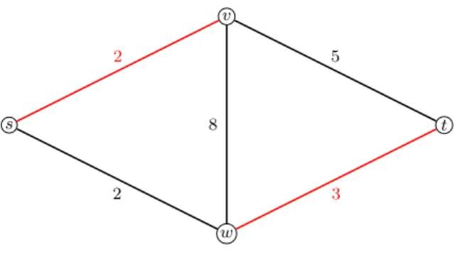
c>1x c>2x
Figure 2.9: Objective function values (c>1x, c>2x) for non-efficient solutions and efficient solutions x∈X.
the solution is obtained as the minimum of Problem (2.6). The number of solutions which can not be obtained by the weighted-sum method can even be of exponential size. In this thesis we are interested in multicriteria problems with an efficient setXE of (pseudo)polynomial size, which can be calculated
in (pseudo)polynomial time. For most of the problems in Section 2.4 the latter requirements are not fulfilled. One exception is the minimum cut problem. Theorem 2.49 ([9]). For a fixed number m of objective functions, the set of efficient solutions XE for the multicriteria minimum cut problem can be
calculated in pseudopolynomial time.
If the set XE has exponential size one may also be interested in
approx-imations of this set, i.e. subsets of XE such that each efficient solution is
approximated by one of the solutions in the subset. Formally the latter ap-proximation concept for multicriteria problems is described as follows. Definition 2.50. For an instance of a multicriteria problem of the form (2.5) with positive objective values c>i x for each feasible solution x ∈ X, we say an algorithm A is anε-approximation algorithm if it calculates a set F ⊆X of solutions such that for each efficient solutionx∈X there exists a solution y∈F with
c>i y≤(1 +ε)c>i x ∀i= 1, . . . , m.
A multicriteria problem has a fully polynomial approximation scheme if for any ε >0 there exists an ε-approximation algorithm whose run-time as well as the maximum size of any number occurring in the computation is bounded by a polynomial inhxi+hεi+1ε. We then say problem (2.5) admits an FPTAS. Note that the polynomial run-time of the algorithm includes that the calcu-lated setF has polynomial size. In literature several approximation methods
have been presented. Two general approaches to obtain approximation algo-rithms are local search methods in the objective space and population based methods ([31]). Furthermore it has been proved that some of the combina-torial problems presented in Section 2.4 admit an FPTAS.
Theorem 2.51([50, 34]). For a fixed numbermof objective functions Prob-lem (2.5) admits an FPTAS for the shortest path probProb-lem, the minimum spanning tree problem and the knapsack problem.
Combinatorial Robust
Optimization
In this section we will give an introduction to the robust optimization frame-work and present a selection of different models which are studied in robust optimization literature.
In many real world applications the input data of an optimization problem can be subject to uncertainty. For example the travel times for the shortest path problem, the traveling salesman problem, or the vehicle routing problem can be uncertain because of unknown traffic situations. Other problems can be influenced by measurement or rounding errors while many financial op-timization problems use information about uncertain demands or uncertain returns of assets.
In the literature there are three main approaches to tackle uncertainty in optimization problems. On the one hand there is the approach of stochastic optimization, which requires a probability distribution on the uncertain data and which aims to optimize the expected value of the objective function [52]. A well known class of stochastical optimization problems are the stochastic two-stage problems where the variables are divided into first-stage variablesx and second-stage variables y. A stochastic two-stage problem is of the form
min
x∈Xf(x) +EP(g(x,˜c))
with feasible set X ⊆ Rn, objective function f : X →
R, a probability
vector ˜c : Ω → Rn with probability distribution
P and EP denoting the
expected value under P. The function g :X×Rn→
R is of the form
g(x, c) = min
y∈Y(x,c)
where c ∈ Rn is any outcome of the probability vector ˜c and Y(x, c) ⊆
Rm is the feasible set which depends on the first-stage solution x and the
outcomec. Hence for each first-stage solution xand each outcomecthe best second-stage solution is selected for a given objective function h and under all feasible solutions Y(x, c). The expected value of this best second-stage value is optimized over all first-stage solutionsx. Often the latter two-stage problem is considered to have uncertainty in the constraints which is modeled by so calledchance-constraints. A chance constraint is of the form
P(f(x,a)˜ > ν)≤α
with f : X ×Rn →
R and given parameters α ∈ (0,1) and ν ∈ R. Here
˜
a : Ω → Rn is another probability vector with probability distribution
P.
If we choose f(x,˜a) := ˜a>x then the chance constraint guarantees that the linear constraint ˜a>x ≤ ν is violated with probability of at most α. One of the main drawbacks of the stochastic optimization approach in practice is to find a probability distribution which models the uncertain data properly. The approach ofdistributional robustnessavoids the latter problem by assum-ing that only the expected value or some other parameters of the unknown probability distribution are given. The objective in this approach is to op-timize the expected value of the worst-case probability distribution under all which have the required parameters [58, 28]. Formally a combinatorial distributionally robust problem is of the form
min
x∈XsupP∈PEP
c>x
(3.1) where P is a set of probability distributions of the probability vector c. Of-ten instead of the linear objective functionc>x other functions are consider e.g. disutility functions (see [42]). The main task in the latter approach is to define theambiguity set P. There are numerous different definitions of ambi-guity sets in literature. Often the set includes only probability distributions which have a given expected value and a given support set. Mostly additional parameters on the probability distribution are required e.g. bounds on given moments, bounds on the probability over given subsets of the support set and many more. A very general definition ofP can be found in [58]. Surprisingly many problems of the form (3.1) for appropriate setsP can be reformulated by using conic optimization duality which yields problems which are often closely related to the robust optimization approach which is mainly studied in this thesis.
The robust optimization approach was first introduced by Soyster [56] in 1973. The idea is to define an uncertainty set U which contains all relevant