University of Wisconsin Milwaukee
UWM Digital Commons
Theses and Dissertations
May 2017
An Integrated Approach for Reliability Evaluation
of Electric Power Systems Considering Natural Gas
Network Reliability
Jiayan Nie
University of Wisconsin-Milwaukee
Follow this and additional works at:https://dc.uwm.edu/etd Part of theElectrical and Electronics Commons
This Thesis is brought to you for free and open access by UWM Digital Commons. It has been accepted for inclusion in Theses and Dissertations by an authorized administrator of UWM Digital Commons. For more information, please [email protected].
Recommended Citation
Nie, Jiayan, "An Integrated Approach for Reliability Evaluation of Electric Power Systems Considering Natural Gas Network Reliability" (2017).Theses and Dissertations. 1518.
AN INTEGRATED APPROACH FOR RELIABILITY EVALUATION OF ELECTRIC POWER SYSTEMS CONSIDERING NATURAL GAS NETWORK RELIABILITY
by Jiayan Nie
A Thesis Submitted in Partial Fulfillment of the Requirements for the Degree of
Master of Science in Engineering
at
The University of Wisconsin-Milwaukee May 2017
ABSTRACT
AN INTEGRATED APPROACH FOR RELIABILITY EVALUATION OF ELECTRIC POWER SYSTEMS CONSIDERING NATURAL GAS NETWORK RELIABILITY
by Jiayan Nie
The University of Wisconsin-Milwaukee, 2017 Under the Supervision of Dr. Lingfeng Wang
With the rapid increase of demand for electric power and the growing complexity of the electric system, the reliable operation of electric systems is facing new challenges. Meanwhile, natural gas has been widely used in transportation, electricity generation, and heating. In addition, gas-fired turbines play a growing vital role in the generation of electricity. However, all the facilities in a natural gas network are subject to failures. The operation of gas-fired turbines will be affected by the status of natural gas network, and the insufficient supply of natural gas may cause the output of gas turbine units to reduce to zero. This power decrease may further influence the operation of power systems. Therefore, it is quite urgent to quantify the influence of natural gas networks on the power system reliability.
A deep understanding of the operation of natural gas network is needed to quantify the impact that natural gas networks will bring to the power system reliability. The main facilities in a natural gas network are natural gas pipelines, compressor stations and natural gas sources. Additionally, the mathematical failure models have been developed for these facilities to build a reliability analysis framework for the gas network. The mass flow of natural gas at different
failure conditions is analyzed by the maximum flow algorithm. Case studies are conducted on a modified Europe Belgium natural gas network to analyze the influences of different failures on the maximum flow of natural gas.
The main problem discussed in this thesis is related to how the natural gas network operation status influences the reliability of power system. The coupling unit is the gas-fired turbine between and electric and gas infrastructures, while the simplified gas-fired turbine model used in this work shows a linear relation among the power generation and the mass flow of natural gas. In this thesis, reliability evaluation is performed based on the hierarchical level II which contains the generation system and the transmission system. The optimal power flow analysis has been conducted for the reliability evaluation. Based on the results of power flow, the status of load shedding can be obtained in a power system. Then, system reliability states can be determined. Failure statuses of both the natural gas network and electric system are simulated by Monte Carlo Simulation. Case studies are conducted on the RTS-79 system and the modified Europe Belgium natural gas network by using MATLAB and IBM CPLEX. The results indicate that the reliability of system decreases.
© Copyright by Jiayan Nie, 2017 All Rights Reserved
TABLE OF CONTENTS
Chapter1 Introduction ... 1
1.1 Research Background ... 1
1.2 Introduction to Power System Evaluation ... 4
1.3 Power System Reliability Analysis Considering Natural Gas Network ... 5
1.4 Research Objective and Thesis Layout ... 6
Chapter2 Natural Gas Network Operation Analysis ... 7
2.1 Introduction ... 7
2.2 Natural Gas Network ... 7
2.3 Natural Gas Network Component Failure Modeling ... 10
2.3.1 Pipeline ... 10
2.3.2 Compressor Station ... 11
2.3.3 Natural Gas Source ... 12
2.4 Methodology of Maximum Flow Algorithm ... 12
2.5 Procedure ... 16
2.6 Numerical Case Study ... 17
2.7 Conclusion ... 23
3. Power System Reliability Evaluation Considering the Influence of Gas Network Failure . 25 3.1 Introduction ... 25
3.2 Gas Turbine Modeling ... 25
3.3 Power System Reliability Evaluation ... 30
3.3.2 Optimal Power Flow ... 33
3.3.3 Methodology of Power System Reliability Evaluation ... 36
3.4 Methodology of Considering the Gas Network into Power System Reliability .... 37
3.4.1 Procedures ... 38
3.5 Case Study ... 41
3.6 Conclusion ... 46
4. Conclusion and Future Work ... 48
4.1 Conclusion ... 48
4.2 Future Work ... 49
LIST OF FIGURES
Figure 1-1 Annual number of incidents………3
Figure 2-1 Natural gas network………9
Figure 2-2 Flow network………..13
Figure 2-3 Flow network with super vertexes………..16
Figure 2-4 Flowchart of natural gas operation analysis………...17
Figure 2-5 Modified Europe Belgium natural gas network……….19
Figure 2-6 Pie chart of maxflow of node 8 in scenario 2……….20
Figure 2-7 Pie chart of maxflow of node 8 in scenario 3……….21
Figure 2-8 Pie chart of maxflow of node 8 in scenario 4……….21
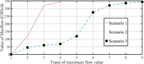
Figure 2-9 Figure 2-9 Types of maximum flow value……….………22
Figure 3-1 Gas-fired turbine model………..27
Figure 3-2 Power system hierarchical levels………...30
Figure 3-3 Two-state model………..32
Figure 3-4 Flowchart of power system reliability evaluation……..………...40
Figure 3-5 Integrated natural gas and power system……….………..42
Figure 3-6 Power generation of bus 22 of scenario 2 (50MW)………...…43
Figure 3-7 Power generation of bus 22 of scenario 3………...43
Figure 3-8 Power generation of bus 7 of scenario 2 (100MW)………..………….……44
LIST OF TABLES
Table 2-1 Basic data of modified Europe Belgium natural gas network………..18
Table 2-2 Network Mass Flow of Scenario 1………20
Table 2-3 Maximum flow value comparison between different scenarios……….22
Table 3-1 Gas-fired turbine parameters………41
ACKNOWLEDGEMENTS
Time flies. It has been eight months since I came to Milwaukee. Life at UWM is truly a challenge, but it is also fantastic. This thesis could not have been completed without the help and guidance of the people around me.
I would first express my gratitude to my advisor Dr. Lingfeng Wang. Dr. Wang led me into this interdisciplinary research field based on his deep understanding of the contemporary power system. He has a unique view and insight toward academic research. It is his encouragement and guidance that helped me break through the obstacles in my research field. His sense of responsibility and passion towards research influenced my greatly. At the same time, I would also like to thank Professor Yu and Professor Zhu for serving on my thesis defense committee and giving me both suggestions and comments about my thesis.
I highly appreciate my advisor of Kaigui Xie in Chongqing University. Without Professor Xie’s help and support, I could not have had the chance to study in the U.S. or to have earned my Master’s degree at UWM.
Special thanks to my classmates: Yingmeng Xiang, Jun Tan, Yanlin Li, Mingzhi Zhang, Zibo Wang, and Qian Wu. In my eight months’ study here, they have provided me a lot of help. I want to especially thank Yingmeng Xiang, a senior student who cooperated with me on my research. His serious attitude towards research, willpower, and wisdom will have a lifelong influence on my attitude towards life.
At last, I want to give my sincere thanks to my family members: Jia Zuo, Jun Nie, my grandmother Yangqin Zhu and my boyfriend Liping Zhou. My family gives me the most powerful support and love. Their selfless love is always my motivation to be a better person. They are always my closet friends and best teachers.
Chapter1
Introduction
1.1
Research BackgroundElectricity is essential to human activities. However, power systems are extremely complex due to factors such as electricity’s inability to be stored effectively in large quantities; the power flow may not follow the path that is wanted by operators but abide physical law; the unpredictable system behavior that may cause domino effects on the entire system; the wide interconnection with other systems; the various physical system size and other reasons. The complexity of the power system brings us a lot of uncertainties, which may cause serious problems to human activities and life. The following are some terrible electricity outages in recent years.
In November 1965, a terrible power outage happened in the U.S. [1]. A 230-kV transmission line tripped and it had a domino effect on the power system which made New York City dark. This blackout impacted 30 million people. Electricity was restored around half of a day.
An even worse blackout happened again in the northeastern United States and northern Canada 38 years later. After one transmission line broke, three other transmission lines switched off, and this further caused a domino effect. 50 million people got a power outage[2]. And this continued for two days. 11 people died and up to 6 billion dollars in damages happened. This incident is the most terrible power outage in North American history[3].
Among Asia, there were also some big electrical outages. On July 31st, 2012, a blackout happened in India. Before the power came on again, almost half of Indians were stuck in the dark for two days. This blackout affected almost 670 million people[4].
As the human society moves forward, the needs for the electricity also increase. The huge increase brings the power system significant challenges. Meanwhile, due to the uncontrolled use of fossil fuel energy, some serious problems emerge such as environment damage, fossil fuel energy shortage, and climate change. At this time, natural gas plays a significant role in meeting the world energy demands [5] due to the following reasons: natural gas is the most clean energy when it is burning; compared to fossil fuel, natural gas is in abundance; natural gas is versatile because it can be used for power generation, heating, vehicle fuel, etc.[6]. After the gas arrives to city gates, it will be delivered to four kinds of loads—residential loads, commercial loads, industrial loads and electric utility[7]. Proven natural gas reserves were around 187.1 trillion cubic meters (tcm) in 2013, which increased 19.5% compare to 2004 levels [8]. Meanwhile, gas-fired turbines started to become popular in power generation for the following reasons: gas-fired turbine-based power plants cost less money compared to other alternatives such as coal fired facilities; the lead time for a gas-fired turbine can be significantly shorter than other alternatives; gas-fired turbines can be extremely efficient and they have less environment impacts.
However, the increasing proportion of gas-fired turbines does not always bring advantages. According to the EGIG ninth report[9], there were 1,309 natural gas pipeline incidents recorded
during 1970-2013 in Europe. From 1994 to 2013, there were 745 serious incidents of natural gas pipelines in the United States, which caused $110,658,083 in property impact.
Figure 1-1 The annual number incidents of Europe during 1970-2013 [9]
The operation status of a natural gas network will have influence on the state of gas-fired turbines because the insufficiency of natural gas supplied to a gas-fired turbine may cause the reduction of generated power, which will further influence the power system’s status, natural gas network’s operation status takes an increasing position in power network reliability evaluation. This threat also caught the North American Electric Reliability Corporation’s attention. From 2011 to 2013, they have been indicating the interconnection of power systems and natural gas networks’ impacts[10]–[12]. All these incidents cause huge physical and economy damage on human society. To reduce these kinds of damages, we need to enhance the power system reliability. Therefore, analyzing power system reliability considering the natural gas network’s influence is quite urgent and significant.
1.2 Introduction to Power System Evaluation
The mechanical failure of power system components is no longer the only factor that will have effects on the power system. Because the fast pace of smart grid, renewable energy, and vehicle technology development, the power system has increased connection with other kinds of systems, components, etc. There are a number of studies that consider new factors in the analysis of power system reliability.
Because the high incorporation of wind energy in the power system, the variable characteristic of wind energy have impacts on the power system reliability. [13] considers this impact that wind turbines will bring to power system. [14],[15], [16] addresses the variability of energy storage(ES) and photovoltaic (PV) in a hierarchical level 1(HL1) power system reliability evaluation. [17],[18] consider adverse weather such as hurricanes that could impact power system reliability significantly. [19],[20] discuss the integration challenges of power system and renewable energy (wind and solar) on power system reliability. [21],[22] consider the availability of natural gas of combined cycle plants that can have influence on power system generation and power system reliability. [23], [24] investigates the impacts of electrical-drive vehicles onto the power system reliability. Because the rapid development of information system among smart grids, [25]–[28] take the higher level cyber security into consideration. [29], [30] consider the wind turbine and information system in an integrated system. [31] considers the influence of controllability and situational awareness on the reliability evaluation.
1.3 Power System Reliability Analysis Considering Natural Gas Network
The most important part to investigate the integrated natural gas and electrical system reliability is how to couple these two systems together. Usually there are two coupling aspects: gas-fired turbine and electric drive compressors. However, there are also other couplings such as energy hubs[32]. Several works are about considering the gas flow in probabilistic power flow. [33] developed an integrated natural gas and electrical networks to operate the power flow. [34] developed a mathematical model to minimize the cost of the integrated network operation. [35] also developed a model for the integrated natural gas and power system considering a distributed slack node and temperature.
As said before, most of the works in this area model a unified power and gas system and does the (optimal) power flow [36]–[39]. Their focus is usually on the gas network reliability. In [40], it discussed a methodology for analyzing natural gas network reliability by following the experience of analyzing the power system. The focus is on the gas network reliability and includes some electric components. However, some works are about investigating the reliability impacts of gas network on power systems in a mathematical way. In [38], it developed a model to analyze the maximum ability of suppling power of the combined-cycle power plants. [41]–[43] analyze the interdependence of electric and gas infrastructure. They analyzed the integrated electrical and gas systems’ reliability.
1.4Research Objective and Thesis Layout
This thesis seeks to consider the influence of the availability of natural gas on the composite power system reliability. Chapter 2 discusses the failure model of natural gas networks and the maximum flow algorithm method that can measure the operation of the network. A case study will be conducted on a modified Belgium natural gas network to indicate the application of the graph theory on flow network. In chapter 3, a gas-fired turbine model will be developed. The methodology of HL II power system reliability evaluation and the detailed procedure of considering the availability of natural gas in the reliability of power system is discussed. A case study will be conducted on the RTS-79 and the modified Belgium natural gas network. Then, chapter 4 will present conclusions and future work.
Chapter2
Natural Gas Network Operation Analysis
2.1IntroductionNatural gas plays a significant role in human activities such as power generation, heating and vehicle fuel. The increasing demand for the natural gas have raised a problem about the reliability of supply.[44]
In the rest of this chapter, section 2.2 introduces the detailed natural gas network; Section 2.3 introduces the failure modeling of gas network, which includes the modeling of natural gas sources, natural gas pipelines, compressor stations. In section 2.4, it discussed the Maximum flow algorithm and its implementation. In section 2.5, Maximum flow algorithm is used to calculate the maximum flow of a real case of modified Belgium gas network in Europe when there were some incidents that occurred inside the network.
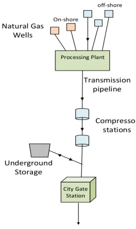
2.2Natural Gas Network
Natural gas networks are somehow similar to power systems in some sense. Both have three parts: production, transmission and distribution. Natural gas comes from wells which are off-shore or on-off-shore. In the well, natural gas tends to flow freely from porous rocks and sandstone. After the natural gas is taken from the well, it needs to be separated from the oil and water to be purified. After the gas goes through a processing plant, it will be compressed and go to the transmission pipeline. Because the long-distance move of the natural gas is accomplished by
pressure, natural gas needs to be pressurized. Next, after arriving at every gas company, the gas will be delivered to every gas loads such as homes, factories, etc.
In our work, we only focus on the operation of natural gas transmission and distribution systems. We did not contain the production system of natural gas. For the natural gas transmission and distribution systems, there are some important components. The natural gas network is as figure 2-1.
1.Natural gas source
Natural gas is in the underground porous rock. Natural gas can be divided into two types in accordance with the existence of the form—associated gas and non-associated gas. Associated gas always coexist with oil, and they can be exploited at the same time from oil fields. Non-associated gas can be directly exploited out in the gas wells. Natural gas wells are always distributed at off-shore or on-shore.
2. Pipelines
Pipelines’ diameters differ from each other in transmission networks and distribution networks. In transmission networks, the diameters’ range is from 15 to 47 inches, while the range for distribution network is from 5 to 15 inches [5]. The main function of these pipelines is transport the natural gas from natural gas wells to deliver companies. Natural gas pipelines are usually buried underground.
3.Compressor stations
Natural gas needs to be highly pressurized when travelling through the long distance transmission network. Due to the friction of the pipelines and natural gas, the pressure of natural gas will reduce over time. Because compressor stations can pressurize the natural gas, compressor stations are placed in gas networks along the pipeline every 40 to 100 mile intervals.
As one can see, natural gas networks are quite complicated because the natural gas can be pressurized and can be stored in pipelines. So, the natural gas flow measurement is also quite complicated. This paper will use a maximum flow algorithm to do the natural gas network mass flow measurement. Processing Plant City Gate Station On-shore off-shore Natural Gas Wells Transmission pipeline Compressor stations Underground Storage
2.3Natural Gas Network Component Failure Modeling
2.3.1 Pipeline
From some industry materials, we can get some real parameters of pipeline like diameter and length. In the GTE report[45], the natural gas pipeline capacity Q has some relationship with pipeline diameter D, which can be described as below:
C~Dη (2-1)
Where:
C is the designed capacity of the natural gas pipeline;
D is the diameter of the natural gas pipeline;
η is a constant conversion coefficient, which is 2.58;
If the parameters of pipeline can be obtained, the designed capacity of natural gas pipeline for a different natural gas pipeline diameter in a gas network can be computed by the formula below [45]: C1 C2 = ( 𝐷1 𝐷2) 𝜂 (2-2) Where:
C1 C2 are natural gas pipelines capacities in comparison;
For the natural gas pipeline failure modeling, if there is an incident happen to a pipeline, there will be a deduction of this pipeline capacity in the model. In this paper, we only consider the total failure to a pipeline which will cause the capacity of this pipeline reduced to zero in this pipeline failure model.
In this paper, the failure probability depends on the length of the pipeline. The European gas transmission pipeline average failure frequency is 3.5×10⁻⁴ per kilometer per year[46]. By knowing the pipeline length, we can obtain the failure probability of these natural gas networks.
2.3.2 Compressor Station
A compressor station is placed in the connection of two natural gas pipelines. For a compressor station, we assume that there is no flow loss or increase under the normal situation inside the compressor station, and it fulfills the flow balance at this compressor station. So, the volume of natural gas of a compressor station is determined by the upper stream, and if there is any incident that occurs in a compressor station, it will have an influence on the volume of both upstream and downstream natural gas. The modeling of compressor station failure is as below.
If any incident occurs in a compressor station, we assumed that this failure of a compressor station will cause a deduction from the pipeline capacity of both upstream and downstream pipelines. More precisely, a failure of a compressor station reduces 20% pipeline capacity of both the inlet pipeline and outlet pipeline. It is assumed that a compressor station annual failure probability is 0.25.[47]
2.3.3 Natural Gas Source
For the natural gas sources, the volume of a source is infinite in a natural gas network, which means the inlet pipeline capacity of a natural gas source is unlimited. For the natural gas sources failure modeling, if there is any failure that happens to a natural gas source, we assumed that this source would not deliver natural gas to this natural gas network anymore, which means the outlet pipeline capacity of a natural gas source will reduce to 0. Here, we assumed the annual failure probability of a gas source is 0.1.
2.4Methodology of Maximum Flow Algorithm
Maximum flow algorithm is one kind of a graph theory. Graph theory can be used as a model to solve some problems for a pipeline network, in which some commodity like gas or water will be transported from one place to another. These networks are usually called flow networks. A gas network is like a flow network. The general problem in such a flow network is to find the maximum flow between two places or the minimum cost of a prescribed flow. These kinds of problems are operation-research problems. Usually, the way to solve them is linear programming. However, the graph theory approach has been found more efficient than linear programming. In this paper, the purpose of analyzing the gas network is to determine the maximum gas flow volume that can afford to gas loads when there is any incident that occurs to natural gas network pipelines, gas sources or compressor stations.
In the graph theory, a flow network is a weighted, connected and simple digraph as Figure 3, described by 𝐺. The line which connects the vertex i and the vertex j is an edge. The numbers
written beside an edge are the edge flow and the edge capacity. An edge capacity Cij can be
thought of the maximum value of the natural gas, which can be transported from vertex i to vertex j along the edge(i,j). The transports happen in a steady state and is measured in units of time. An edge flow fij can be thought of the current static flow amount which fulfills a specific distance edge at one second.
s 1 2 3 4 5 t 8 6 7 5/20 3/8
Figure 2-2 Flow network
In this figure, 𝑠, 𝑡, 𝑣𝑖 are three kinds of vertexes. 𝑠 represents the source vertex, from which these flows inside the network come. 𝑡 is the sink vertex, into which these flows finally go. 𝑣𝑖
is intermediate vertex.
Among the flow network, the flow must satisfy following conditions: 1. For an edge (i, j) in G,
2. For a source vertex s in G, ∑ 𝑓𝑠𝑖 𝑖 − ∑ 𝑓𝑖𝑠 𝑖 = 𝑤 (2-4)
Where w is the value of the flow. 3. For a sink vertex 𝑡 in G,
∑ 𝑓𝑡𝑖 𝑖 − ∑ 𝑓𝑖𝑡 𝑖 = −𝑤 (2-5)
4. For an intermediate vertex 𝑣𝑖𝑗
∑ 𝑓𝑗𝑖 𝑖 − ∑ 𝑓𝑖𝑗 𝑖 = 0 (2-6)
Equation (2-3)indicates that any flow inside an edge cannot exceed its capacity. The rest of the conditions state that an inlet flow of a flow network from a source is 𝑤, an outlet flow of a flow network into a sink is 𝑤, and at every intermediate vertex, the flow is conserved. We can find that 𝑤 also represents the value of the flow from vertex s to vertex 𝑡.
So, the problem can be described in this way: if any incident happens to any edge or any vertex in this network, what is the maximum amount of the natural gas flow which comes from a given vertex s that can be sent to a specified vertex t via the entire flow network?
In a given flow network G, the maximum value of a flow from s to 𝑡 is equal to the minimum value of the capacities of all the cuts in G that separate s from 𝑡. A cut-set is what separates the source s from sink 𝑡. Such a set of edges in flow network is a 𝑐𝑢𝑡
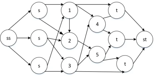
The max-flow min-cut theory is applicable to a flow network with one source node and one sink node. However, in a practical natural gas network, there cannot be only one source node and one gas load, which means in the graph theory, that there are multiple vertices for s and t. In order to apply maximum flow algorithm to these kinds of practical natural gas networks, we can extend the max-flow min-cut theory appropriately.
If there is one flow network with 𝑠1, 𝑠2, 𝑠3, … , 𝑠𝑚 sources and 𝑡1, 𝑡2, 𝑡3, … 𝑡𝑛 sinks, the flow of any source node can be delivered to any sink node among the entire flow network. Then we just need to set a super source node and a super sink node. A super source node connects to all the original source nodes. The capacity of these edges is unlimited. The original sink nodes connect to a super sink vertex, and the capacity of these edges is unlimited. The advanced network looks like figure 4. In this way, the maximum flow problem from which all the original sources to all the sink nodes then can be explained in this way: if there is any incident to any edge or any vertex in this network, find the maximum amount of the natural gas flow that can be sent to a super sink t which comes from a super source s via the entire flow network.
ss s s s 2 3 st t t t 1 4 5
Figure 2-3 Flow network with super vertexes
2.5Procedure
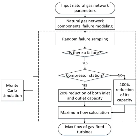
Natural gas network failure simulation and evaluation are based on the software of MATLAB. The procedures are as following:
1) Input a natural gas network information such as node number, diameter, pipeline length, etc.
2) Failure modeling of natural gas sources, natural gas pipelines and compressor stations. Calculate the failure probability of all the components.
3) Random sampling all the natural gas sources, natural gas pipelines and compressor stations by Monte Carlo simulation.
4) If there is any failure happen to a natural gas source and natural gas pipeline, both of their capacity reduce to 0; if there is any failure happen to a compressor station, there is a 20% deduction of both inlet and outlet pipeline capacity of a compressor station. 5) Based on step 4, calculate the max mass flow of all the natural gas loads by using the
Natural gas network components failure modeling
Random failure sampling
Compressor station?
YES
20% reduction of both inlet and outlet capacity
NO 100% reduction of its capacity Is there a failure? YES
Maximum flow calculation
Max flow of gas-fired turbines
Input natural gas network parameters
Monte Carlo simulation
Figure 2-4 Flowchart of natural gas operation analysis
2.6Numerical Case Study
This section is about the natural gas network failure simulation study. For this section and the case study in chapter 4, the natural gas networks are all modified Europe Belgium natural gas network[48]. In the following, we will use ‘system M’ to represent this modified Europe Belgium natural gas network.
As discussed before, the failure of a natural gas network can occur among three components—
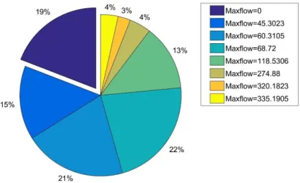
all the probable fail components in different scenarios. We assume that node 8 connects a gas-fired turbine. We want to figure out that if any failure happens, what is the maximum value of the natural gas that this network can supply to this node. Based on the different failure scenarios, we can indicate the influences of these failure scenarios on the gas-fired turbines by calculating the value of the maximum flow. The case study is conducted on the software MATLAB, using Monte Carlo simulation, which be discussed in chapter 3, for the random failure of three components. Theiteration sets to 100,000 times.
Table 2-1 shows the modified Europe Belgium natural gas network basic data. The network is as figure 2-5.
Table 2-1 Basic data of modified Europe Belgium natural gas network
From To Diameter(mm) Length(km) Technical physical capacity(GWh/d) 1 2 890 4 343.6 2 3 890 6 343.6 3 4 890 26 343.6 5 6 590.1 43 118.5306 6 7 590.1 29 118.5306 7 4 590.1 19 118.5306 4 8 890 55 343.6 9 10 890 5 343.6 10 11 890 20 343.6 11 12 890 25 343.6 12 13 890 42 343.6 13 14 890 40 343.6 14 8 890 5 343.6 8 15 890 10 343.6 15 16 890 25 343.6 12 17 395.5 10.5 42.04772 17 18 315.5 26 23.41755 18 19 315.5 98 23.41755 19 20 315.5 6 23.41755
01 02 03 04 07 05 06 08 16 15 14 13 12 11 10 09 17 18 19 20
Figure 2-5 Modified Europe Belgium natural gas network
For the case study, there are four scenarios as below: Scenario 1 Normal operation situation without failure Scenario 2 Natural gas pipelines’ failure
Scenario 3 Natural gas pipelines and compressor stations’ failure Scenario 4 All the components’ failure
Table2-2 Network Mass Flow of Scenario 1
End Nodes Flow End Nodes Flow
1 2 2 3 3 4 4 8 4 22 5 6 6 7 7 22 8 15 9 10 10 11 11 12 12 13 343.6 343.6 343.6 225.07 118.53 118.53 118.53 118.53 343.6 141.95 141.95 141.95 118.53 12 17 13 14 14 8 15 16 16 22 17 18 18 19 19 20 20 22 21 1 21 5 21 9 23.418 118.53 118.53 343.6 343.6 23.418 23.418 23.418 23.418 343.6 118.53 141.95
Figure 2-7 Pie chart of maxflow of node 8 in scenario 3
Figure 2-8 Pie chart of maxflow of node 8 in scenario 4
From the pie charts of three different scenarios, we can find that different scenarios have different categories of maximum flow value. If we only consider the failure of the natural gas pipeline, there are only three kinds of results. For the scenario 2 and scenario 3, there are eight kinds of maximum value results, which be showed in figure 2-6. The increase of the categories of the maximum flow value mostly caused by the consideration of the compressor station. The failure of the natural gas source and pipelines deduce the capacity to 0. However, the failure of
a compressor station only cause 20% decrease on capacity which increases the variability of the flow value.
Figure 2-9 Types of maximum flow value
The differences of the maximum and minimum value between the basic value of different scenarios are showing in the table below:
Table2-3 Maximum flow value comparison between different scenarios
Basic Minimum Maximum Difference (%)
Pipeline 118.53 0 320.1823 100~170
Pipeline and compressor
118.53 0 335.1905 100~180
All the components 118.53 0 335.1905 100~180
2.7Conclusion
In this chapter, we have introduced the main components of natural gas network—natural gas sources, transmission pipelines, compressor stations, metering stations, etc. From the source to the demand, natural gas network can be divided to generation, transmission and distribution, which are very similar to power systems.
We also discussed the natural gas network failure modeling for the three main components— natural gas pipelines, compressor stations and natural gas sources. According to some industry reports, we can obtain the relationship of pipeline diameter and pipeline capacity. For the failure modeling of pipelines, we assume that the failure of any pipeline will cause the pipeline capacity to decrease to 0. For the compressor failure modeling, we assume that the failure of any compressor station will have a 20% reduction on both inlet and outlet pipeline capacity. For the failure modeling of gas sources, it is assumed that a failure of a source would not deliver natural gas anymore. The annual failure probability or frequency of these three components can be obtained from some industry reports.
Then, we have discussed the theory of maximum flow algorithm. Maximum flow algorithm is used to find the maxflow from source node s and sink node t via the entire flow network. For a natural gas network that has multiple sources and sink nodes, like a natural gas network, we can use a super source and a super sink node to adjust the original algorithm for appropriate use.
Next, we introduce the procedures of the natural gas network failure evaluation, and give the flow chart. At first, we need the network parameters to build the components failure model. By using Monte Carlo simulation on MATLAB, we can obtain the maximum flow of all the gas loads.
Finally, we performed a failure case study in a modified Europe Belgium natural gas network by using a maximum flow algorithm. The Monte Carlo simulation runs 100,000 times. All the results of maximum flow of node 13 have been divided into 9 areas showing the frequency of different period maxflow intervals.
3.Power System Reliability Evaluation Considering the Influence
of Gas Network Failure
3.1Introduction
In recent years, there has been a concentration on the power system reliability. As discussed in chapter 1, very few people focus on the influence of a gas network failure that will bring to the power system.
In the rest of this chapter, section 3.2 introduces the modeling of a gas-fired turbine; Section 3.3 introduces the evaluation of the power system reliability, in which, section 3.3.1 introduces the methodology of power system reliability evaluation, and section 3.3.2 introduces a consideration of the influence of a natural gas network into the power system reliability evaluation. Section 3.4 shows the procedure of section 3.3.2. Section 3.5 is the conclusion of this chapter.
3.2Gas Turbine Modeling
Gas turbines act as the couplings of a natural gas network and the power system. In the natural gas network, gas turbines need natural gas to operate regularly. They are gas demand nodes. At the same time, in the power system generation, gas turbines can use natural gas to generate power. In this work, we only focus on the gas turbine while there are also other couplings like electrical-driven compressors or energy hub which can connect gas networks and the power system together. We only focus on how a natural gas network will influence the power system.
Various kinds of gas turbines have been used in industry and air aspects for many years. The most used gas turbines for power generation are single shaft gas turbines. This kind of gas-fired turbine is composed of three main parts, as figure 8 shows: an air compressor, a combustion chamber, and a turbine. For a single shaft gas turbine, the air compressor and the turbine are on one shaft. The turbine provides the power for both the load and the air compressor. First, the air around a gas turbine is absorbed into the air compressor. At the compressor section, all of the air molecules are squeezed together. As the air is squeezed, it gets hotter and the pressure increases. Next, natural gas which comes from a natural gas network is injected into the combustion chamber, where it is mixed with the hot air which comes from the air compressor and is burned at a (ideally) constant pressure. Next, the hot gas goes into a turbine, where it expands. The turbine then captures the energy from the expanding gas and provides the necessary energy for the operating of an air compressor. The chemical energy is converted to mechanical energy. The leftover energy drives the shaft which connects to a generator to rotate. The fast rotating shaft can generate power. In this way, the mechanical energy is converted to electrical energy.
From the brief introduction, we can find that the power generation is related to many factors, such as the air temperature, pressure, the compression ratio, etc. And the modeling of a gas turbine also can be divided into three parts, which are air compressor modeling, combustion chamber modeling and turbine modeling.
Air compressor Combustion chamber Turbine Air Natural gas Exhaust Generation Electricity
Figure 3-1 Gas-fired turbine model
In our work, we only focus on the relationship between a natural gas network and power system because we want to analyze how the natural gas mass flow will influence the power generation in a gas-fired turbine. The accurate model is too complicated for this work and cannot indicate the relationship clearly. So, we simplified the gas-fired turbine modeling. About the gas-fired turbine, there are a lot of ways to build the model[49]–[51]. However, they are way too far from this thesis’s purpose. We do not consider the environmental changes and we assumed the cycle inside a gas-fired turbine is ideal, which means the pressure and the temperature would not change separately in the three main parts. Base on the above simplification, we can obtain the direct relationship between the mass flow of the natural gas and the power generation.
−𝑊 ∗ 𝐶𝑝𝑎(𝑇2− 𝑇1) + 𝑊 ∗ 𝐶𝑝𝑒(𝑇3− 𝑇4) = 𝑃 (3-1)
Where 𝑊 is the sum of mass flow rate of natural gas 𝑊𝑓 and air 𝑊𝑎, 𝑊 = 𝑊𝑓+ 𝑊𝑎; 𝐶𝑝𝑎, 𝐶𝑝𝑒
is the heat capacity of air and natural gas separately; 𝑇𝑖 is the temperature at different points inside a gas turbine. ‘1’ is at the inlet of the air compressor, ‘2’ is at the outlet of the air compressor and the inlet of the combustion chamber. ‘3’ is at the inlet of the turbine and the outlet of combustion chamber. ‘4’ is at the outlet of the turbine. 𝐻𝑢 is the lower heating value
of the natural gas. 𝑃 is the power generation of the gas turbine.
This formula describes the energy conversion inside a gas turbine. At the air compressor, the compression of air supplies the energy to increase the air pressure and temperature. In the combustion chamber, the burning of mixed air and natural gas will release a lot of thermal energy, which will make the turbine shaft rotate in the turbine. That thermal energy is described by the temperature decrease in the turbine. Natural gas will directly be delivered to the combustion chamber, which is the most important part in our modeling. If an incident happens in a natural gas network, it will cause a natural gas flow deduction to a gas turbine. From formula (3-2) we can know that the deduction of the natural gas mass flow will influence the temperature. It will further influence the power generation.
The relationships between temperature and other parameters are described below [52]:
𝐶𝑝𝑒(𝑇3− 𝑇2) = 𝐻𝑢 ∗
𝑊𝑓
Where 𝑝i is the pressure at different points inside the gas turbine; 𝜂𝑐, 𝜂𝑡 is the efficiency of the
compressor and turbine separately; and σ is a constant 1.4.
In this thesis, we assume that the pressure at each point remains a constant value, therefore, (3-3) and (3-4) can be written as:
𝑇
2− 𝑇
1=
𝑇
1𝜂
𝑐∗ 𝐾
1 (3-5)𝑇
3− 𝑇
4= 𝑇
3∗ 𝜂
𝑡∗ 𝐾
2 (3-6)From formula 3-1 to 3-4, we can obtain the relationship of power generation and natural gas mass flow: 𝑃 𝑊 = − 𝐶𝑝𝑎𝑇1 𝜂𝑐 𝐾1+ 𝐶𝑝𝑒𝜂𝑡(𝐻𝑢𝑊𝑓 𝑊𝐶𝑝𝑒 + 𝑇1+𝑇1 𝜂𝑐 𝐾1) 𝐾2 ( 3-7)
Because we simplified the gas turbine modeling, the relationship is linear. In fact, the operation of a gas-fired turbine will be influenced by a lot of other variables such as the temperature or ambient environments. In this paper, we only focus on the direct influence of a natural gas network on the power system, which can be described by the relationship of natural gas mass flow 𝑊𝑓 and power generation 𝑃.
𝑇
2− 𝑇
1=
𝑇
1𝜂
𝑐[(
𝑝
2𝑝
1)
𝜎−1 𝜎− 1]
(3-3)𝑇
3− 𝑇
4= 𝑇
3∗ 𝜂
𝑡∗ [1 − (
𝑝
4𝑝
3)
𝜎−1 𝜎]
(3-4)3.3Power System Reliability Evaluation
As discussed in chapter 1, power system is complicated. The system status can be changed by many factors. Therefore, to maintain a reliable power system, it is useful to discuss the system status.
From the function of a power system, it can be divide into three parts, which are generation system, transmission system and distribution system. For the power system reliability study, a power system usually be divided to three parts—hierarchical level I (generation system), hierarchical level II (composite generation and transmission systems), and hierarchical level III (complete system including distribution systems) as the figure 3-2 below. These three hierarchical levels also indicate the ability to satisfy these subsystems’ function. HL I need to satisfy the pooled system demand; HL II needs to deliver energy to the transmission system supply points and the HL III needs to fulfill the individual consumers’ capacity and energy demands. Generation facilities Transmission facilities Distribution facilities Hierarchical level I Hierarchical level II Hierarchical level III
When we talk about the power system reliability, we always consider the secure, adequate of a system and focus on the system status. Therefore, power system reliability includes system adequacy and system security. System adequacy indicates the ability of the system facilities to fulfill the consumer demand among the system. These facilities always considered as the facilities that can generate energy and transport the energy to load demand points. System adequacy is in static conditions while system security is just opposite. Whenever there is any disturbance occurring within a system, the ability to respond to that disturbance is called system security. Therefore, system security is no longer in static conditions, it needs to response to any disturbance. In this thesis, we only consider the system adequacy among HL II systems.
3.3.1 Monte Carlo Simulation
There are two different approaches to evaluate power system reliability and natural gas network: simulation methods and analytical methods. In this thesis, a simulation method Monte Carlo simulation(MCS) is used to assess the power system reliability and natural gas network failure operation[53]. Due to the similarity of the natural gas network and the power system, basic concepts, principles and procedures of MCS utilized on both systems are almost the same. Therefore, in this section, we mainly introduce the application of MCS on power system.
Simulation methods are totally using random numbers which are generated by computer software. Every component in a system will follow a random nature of the processes. So, even the same systems will have different behavior patterns after a period of operation. A specific
system could behave as any of these behavior patterns. Simulation methods are aiming to inspect and predict these behavior patterns during a simulation time. Based on these patterns, we can obtain a large number of reliability parameters, then we can obtain the reliability indices distribution such as LOLE, LOEE, LOLD, etc.
In this thesis, we mainly focus on the HLII power systems which include generation and transmission systems. For the units in these two systems, a two-state representation is used. These two states are up and down. ‘Up’ means this unit operates in normal condition. ‘Down’ indicates that this unit cannot operate as usual and it is in a failure condition. In the reliability study, we use 0 to represent ‘Up’ state, and use 1 to represent ‘Down’ state. Being in ‘UP’ state and ‘DOWN’ state have the identical probability just as unavailability and availability. Modeling a two-state unit state is quite simple for MCS. It only needs to generate a random number k between 0 and 1, then compare the number k with the unit’s failure probability P. If k < P, then the unit is in ‘DOWN’ state; if k>= P, then the unit is in ‘UP’ state.
Unit up 0 Unit down 1 λ μ
3.3.2 Optimal Power Flow
3.3.2.1Optimal Power Flow Overview
The reliability evaluation of the composite power system must base on the power flow analysis. We want to make the most economic investment to increase the reliability of power system. However, the most economic dispatch may exceed the limitation of flows or voltages. Optimal power flow is to find the optimal solution of an objective function considering some constraints of power system[54]. The most common objective function is to minimize the cost of generation. Meanwhile, there are also other objective functions such as minimize system losses or minimize changes in controls. In this research, the objective function is to minimize the load curtailment. The power system constraints include equality constraints and inequality constraints. Equality constraints are the power balance at each node, while inequality constraints are network operation limits and some other control variables’ limits. Control variables usually are active power output of the generating units, voltage at the generating units, position of the transformer taps, etc. These variables are represented by vector 𝑢. Responses of the system to the changes of the control variables are described by state variables. State variables are magnitude of voltage at each bus except generator busses and angle of voltage at each bus except slack bus. These variables are represented by vector 𝑥.
3.3.2.2Mathematical Formulation of the OPF
All the variables, constrains and objective function can be described by mathematical formulations as below:
Objective function: 𝑓 = min u ∑(𝑃𝐶𝑗) 𝑁𝐷 𝑗=1 (3-8) Equality constraints: 𝑃𝑗𝐺 − 𝑃𝑗𝐿 = ∑ 𝑉𝑗𝑉𝑖[𝐺𝑗𝑖cos(𝜃𝑗− 𝜃𝑖) + 𝐵𝑗𝑖sin(𝜃𝑗 − 𝜃𝑖)] 𝑁 𝑖=1 (3-9) 𝑄𝑗𝐺− 𝑄𝑗𝐿 = ∑ 𝑉𝑗𝑉𝑖[𝐺𝑗𝑖sin(𝜃𝑗 − 𝜃𝑖) + 𝐵𝑗𝑖cos(𝜃𝑗 − 𝜃𝑖)] 𝑁 𝑖=1 (3-10) 𝑗 = 1, … , 𝑁
These equality constraints can be represented by:
𝑔(𝑢, 𝑥) = 0 (3-11)
Inequality constraints:
Voltages operating limits
𝑉𝑗𝑚𝑖𝑛 ≤ 𝑉𝑗 ≤ 𝑉𝑗𝑚𝑎𝑥 (3-12)
Power flow operating limits
|Fij| ≤ 𝐹𝑖𝑗𝑚𝑎𝑥 (3-13)
Control variables limits
𝑢𝑗𝑚𝑖𝑛 ≤ 𝑢𝑗 ≤ 𝑢𝑗𝑚𝑎𝑥 (3-14)
These inequality constraints can be represented by:
In this thesis, we will linear these equations by DC power flow approximation for a fast analysis. We will do a number of approximations. For the power flow equations, if we only consider the DC power flow, there is no reactive power. So, the equality constraints can be described as:
𝑃𝑗𝐺 − 𝑃𝑗𝐿 = ∑ 𝑉𝑗𝑉𝑖[𝐺𝑗𝑖cos(𝜃𝑗− 𝜃𝑖) + 𝐵𝑗𝑖sin(𝜃𝑗 − 𝜃𝑖)] 𝑁
𝑖=1 (3-16)
For DC power flow, the resistance of the branches can be neglect, formula 3-16 can be adjusted to:
𝑃𝑖𝑗 = ∑ 𝑉𝑗𝑉𝑖𝐵𝑗𝑖sin(𝜃𝑗 − 𝜃𝑖)
𝑁
𝑖=1 (3-17)
Assume that the voltage magnitudes are 1 p.u., then the formula change to:
𝑃𝑖𝑗 = ∑ 𝐵𝑗𝑖sin(𝜃𝑗− 𝜃𝑖)
𝑁
𝑖=1 (3-18)
Assume that all angles are very small, the formula can be simplified as:
𝑃𝑖𝑗 = ∑ 𝐵𝑗𝑖(𝜃𝑗− 𝜃𝑖) = ∑ 𝜃𝑗− 𝜃𝑖 𝑥𝑗𝑖 𝑁 𝑖=1 𝑁 𝑖=1 (3-19)
Therefore, the optimal power flow can be described as:
min
u 𝑓(𝑢, 𝑥)
𝑠. 𝑡. 𝑔(𝑢, 𝑥) = 0 ℎ(𝑢, 𝑥) ≤ 0
(3-20)
By doing the optimal power flow, we can know the real power supplying status at each load bus among the whole power system, which can be used to analyze the system reliability furthermore.
3.3.3 Methodology of Power System Reliability Evaluation
For the generation systems reliability evaluation, the most used parameter is unavailability. Unavailability is a probability that can figure out the component on forced outage during a period of time in the future. It is also known as forced outage rate (FOR).
Unavailability = U = λ λ + μ= 𝑟 𝑚 + 𝑟 = 𝑀𝑇𝑇𝑅 𝑀𝑇𝑇𝐹 + 𝑀𝑇𝑇𝑅 = ∑[𝑢𝑝 𝑡𝑖𝑚𝑒] ∑[𝑑𝑜𝑤𝑛 𝑡𝑖𝑚𝑒] + ∑[𝑢𝑝 𝑡𝑖𝑚𝑒] (3-21) Availability = A = μ λ + μ= m m + r= 𝑀𝑇𝑇𝐹 𝑀𝑇𝑇𝐹 + 𝑀𝑇𝑇𝑅 = ∑[𝑢𝑝 𝑡𝑖𝑚𝑒] ∑[𝑑𝑜𝑤𝑛 𝑡𝑖𝑚𝑒] + ∑[𝑢𝑝 𝑡𝑖𝑚𝑒] (3-22)
Where λ is the expected failure rate; μ is the expected repair rate; m is the mean time to failure. It also known as MTTF, which equals to1/λ; r is the mean time to repair. It is also known as MTTR, which equals to 1/μ; m + r is the mean time between failures.
In our thesis, the probability of transmission facilities that on forced outage during one year is similar to the generation:
𝑃 =𝑜𝑢𝑡𝑎𝑔𝑒 𝑑𝑢𝑟𝑎𝑡𝑖𝑜𝑛
8760 ∗ 𝜆 (3-23)
These equations are applicable to a unit of a two-state model. Assume that there are N components in a power system, every component has two states. Then there are 2N states
load indices and loss of energy indices are developed. In this thesis, we use the Loss of Load Probability (LOLP) and Expected Energy Not Supply (EENS) to indicates the system reliability status. LOLP is the probability that a system available capacity cannot suffice the customer demands in a period of time. And EENS is the expected energy that a system available capacity cannot suffice the customer demands in a period of time.
3.4Methodology of Considering the Gas Network into Power System Reliability
As discussed in 3.2, the coupling of a natural gas network and a power system is a gas-fired turbine. We have already talked about the failure modeling of the natural gas network. Maximum flow algorithm is used to calculate the maximum mass flow that can be delivered to a gas-fired turbine when there is any incident that occurs inside a natural gas network. For a gas-fired turbine, there are two ways to fail, one is the mechanical problem, which means this is a self-dependent reason. Another way to fail is that there is not enough natural gas supply to a gas-fired turbine. Here, we roughly say this is caused by the natural gas network. So, when we do the Monte Carlo simulation of power system generators, samplings of gas-fired turbines can be divided into two parts.
The first part is a two-state sampling. There are only ‘0’ and ‘1’ states of a gas-fired turbine.’0’ means this turbine is operating as usual and ‘1’ means a failure occurred and it does not generator any power, it is down. This part is sampling the mechanical reason of gas-fired turbine itself.
The second one is multiple states sampling. The state of a gas-fired turbine is not only a two-state anymore. By randomly sampling a failure(s) of a natural gas network, we can obtain the value of natural gas mass flow of gas-fired turbines by Maximum flow algorithm. Referring to the gas-fired turbine model, there is a linear relationship between natural gas mass flow and power generation, which means, by different values of natural gas mass flow, we can obtain different value of power generation. So, the sampling of this part will follow this linear relationship. By the different value of natural gas mass flow, we adjust the power generation to the corresponding value.
Because those two failure reasons are independent from each other, the two sampling parts will be done at the same time and separately. In this chapter, Monte Carlo simulation of a natural gas network failure sampling and a power system failure sampling will be taken at the same time inside an integrated system.
3.4.1 Procedures
The procedures are described as follows:
1) Model all the generators, branches and buses in a power system.
2) Model all the pipelines, natural gas sources and compressor stations of a natural gas network. This model was discussed in section 2.3 of chapter 2.
3) Calculate reliability parameters such as failure probability of generators and transmission lines in a power system by using calculation equations of (3-21)-(3-23).
4) Do the optimal power flow of this power system. Optimal power flow equations refer to (3-8)-(3-20)
5) Randomly sample the failure of all the branches and generators including the gas-fired turbine. If they are down, their status will be adjusted to ‘1’.
6) Randomly sample the failure of a natural gas network. Any failure that occurs in a natural gas network will influence the value of natural gas mass flow.
7) Calculate the maxflow of gas-fired turbines which are also power generators in a power
system by using the Maximum flow algorithm
8) Calculate gas-fired turbines’ power generation refer to the gas-fired turbine model by using the max mass flow obtained in step 7.
9) Check the value of power generation. If it is under 20% of its max generation, this gas-fired turbine is down, the status will be adjusted to 1 and the generation output is 0; if the value is over 20% of its max generation, adjust the original generation output to this value, this gas-fired turbine status remaining ‘0’.
10)Calculate the optimal power flow again by using the newest power system parameters. 11)Calculate the reliability indices of LOLP and EENS
Step 1 Power system modeling
Step 2 Gas network modeling
Step 3 Reliability parameter calculating
Step 4 Optimal power flow
Step 5 Random sampling the failure of power system
Step 6 Random sampling the failure of natural gas network
Step 7 Calculate the maxflow of gas-fired turbines
Step 8 Calculate the power generation of gas-fired turbines
Step 9 Status of Generators check and adjust
Step 10 Optimal power flow
Step 11 Calculate Reliability indices LOLP EENS
Monte Carlo simulation
3.5Case Study
For the case study, we conduct it on the same modified Europe Belgium natural gas network as chapter 2 and the RTS-79 system for power system[55]. Here, we assume that node 8 and node 13 in the natural gas system M is a gas-fired turbine respectively. These two gas-fired turbines also are generators in power system. Node 8 connected to Bus 22. Node 13 connected to Bus 7. The maximum power generation of bus 22 and bus 7 is 50MW and 100MW respectively. The parameters of gas-fired turbine are as table 3-1. The integrated network is as figure 3-5.
Table 3-1 Gas-fired turbine parameters
Parameter Meaning Value
Hu Low heat value 47451
Cpa Heat capacity of air 1.005
Cpe Heat capacity of natural gas 2.4906
T1 Temperature 288.15
eff_c Efficiency of air compressor 0.85
eff_t Efficiency of turbine 0.89
Wa Mass flow rate of air 5000
K1 Constant parameter 2.02419
K2 Constant parameter 0.505976057
For this case study, we consider three different scenarios: Scenario 1 Basic power system
Scenario 2 Consider the natural gas transmission system and distribution system Scenario 3 Consider the whole natural gas system including natural gas sources
Figure 3-6 Power generation of bus 22 of scenario 2 (50MW)
Figure 3-8 Power generation of bus 7 of scenario 2 (100MW)
Table 3-2 Reliability indices
LOLP Difference EENS Difference
Basic power system 0.0904977168949 77 1.296723118395446e+05 Integrated system without natural gas source 0.1087945205479 45 +20.2179% 1.580310437448405e+05 +21.8695% Integrated system with natural gas source
0.1152420091324 20
+27.342% 1.678123731976062e+05 +29.4126%
From figure 3-6 to figure 3-9, these figures show the output generation distribution of bus 22 and bus 7. In figure 3-6 there are only 4 kinds of power output value, but the value increase to 5 if consider the natural gas source failures as figure 3-7. The multiple states of power output are due to the multiple status of compressor stations’ capacity and the liner relationship of natural gas mass flow and the output of gas-fired turbines.
From the power generation of different scenarios among these two buses, it can be indicated that although the influence of consider the natural gas sources on the mass flow in chapter 2 case study seems very tiny, it makes a large difference in power generation output. From the table 3-3, we can indicate that the failure of natural gas network will decrease the reliability of power system. If we consider the influence of natural gas network failures except the natural gas sources, the power system loss of load probability will increase 20.22%, and expected energy not supply will increase 21.87%. If we consider the influence of natural gas network
failures include natural gas sources, the power system loss of load probability will increase 27.34%, and expected energy not supply will increase 29.41%.
3.6Conclusion
In this chapter, first, we introduced the gas turbine modeling. A gas turbine is composed of an air compressor, a combustion chamber and a turbine. Gas turbine modeling is based on the entire gas turbine energy transformation. Air compressor will pressurize the air and then send it to the combustion chamber. There, mixed air and natural gas will be fired and the increased temperature will make the turbine shaft rotate. The chemical energy changes to mechanical energy. From the model, we can obtain the clear relationship between the mass flow of natural gas and power generation. We also discussed how to obtain the basic parameters in this model.
Then, we introduced the basic reliability evaluation theory. We introduced some reliability concepts such as unavailability and failure probability. Some reliability indices such as loss of load indices LOLP and loss of energy indices EENS that are used in this paper are introduced. The reliability model in this paper is based on the two-state model. Components only have two states: ‘Up’ or ‘Down’.
After introducing the background of reliability evaluation, we consider the natural gas network in the power system reliability evaluation. The coupling is the gas fired turbine. By using the natural gas network failure model and maximum flow algorithm, we can simulate the failure of a natural gas network and obtain the maximum mass flow of gas-fired turbines. A failure of
a gas fired turbine has two independent causes—mechanical failures and natural gas network failures. So, the sampling for gas fired turbines is divided into two separate parts. Then, random sample the power system including all the generators and branches, run the Monte Carlo simulation, calculate the optimal power flow and load cut. Finally, we can obtain the reliability indices such as LOLP and EENS.
4.Conclusion and Future Work
4.1ConclusionThis thesis is mainly about indicating the influence of failures of natural gas networks on the power system reliability evaluation.
As the usage of gas-fired turbines in the power system increases, the supply of natural gas to gas-fired turbines will affect the power generation. This result means that the natural gas network status has some negative effects on the power system. If any failure occurs in a natural gas network, it may cause power system outages. However, this influence is still considered less in power system reliability evaluations. Therefore, consideration of the natural gas network status in power system reliability evaluations is urgent and significant.
Next, the main components of the natural gas network have been introduced. Natural gas networks are very similar to power systems because both of them can be divided into
generation, transmission and distribution. Failure modeling of natural gas sources, natural gas pipelines and compressor stations were made for the evaluation of natural gas network
operation. Maximum flow algorithm of graph theory was used to measure the mass flow of natural gas whenever there was any failure in a natural gas network. A modified Belgium natural gas network was used in a numeric case study. Monte Carlo simulation was used to simulate the failure of the natural gas network based on the software MATLAB. Numbers of maxflow were obtained in variable network status.
The coupling of the power system and natural gas network we discussed in the thesis was gas-fired turbine. A gas turbine is composed of an air compressor, a combustion chamber and a turbine. Gas turbine modeling is based on the entire gas turbine energy conversion, where chemical energy is converted to mechanical energy by air compression and burning. Mechanical energy is converted to electrical energy by the rotating of the turbine shaft. Based on the simplified gas-fired turbine, we can obtain a linear relationship between the natural gas mass flow and the power generation. Here, we already have the failure model of natural gas networks. We can use the maximum flow algorithm to calculate the mass flow of natural gas. By knowing the relationship between natural gas mass flow and power generation, the failure of natural gas networks is considered in power system reliability evaluation. Some reliability indices such as loss of load indices LOLP and loss of energy indices EENS are used to indicate the system reliability status. Results indicate that the consideration of natural gas network failure will decrease the reliability of power system to some degree.
4.2Future Work
In this research, the focus is mainly on the power system reliability. However, the interconnection of power system and natural gas network means that electric grid also has an influence on the natural gas network. Focus can be put on the integrated system analysis, and we can do the optimal power flow in the integrated system. Additionally, there is still room for further extending the proposed models and algorithms. The modeling for the natural gas network can be more accurate by using hydraulic gas turbine models. The model of gas-fired
turbines used in this work was simplified. In fact, gas-fired turbines’ performance will be influenced by environment parameters such as inlet gas temperature and inlet gas pressure. In order to obtain a more accurate relationship between natural gas mass flow and power generation, an accurate gas-fired model should be developed.
References
[1] G. D. Friedlander, “What went wrong VIII: The Great Blackout of ’65: Could the long
night happen again? What was learned from the dramatic six-state (plus Ontario) outage of November 10, 1965?,” IEEE Spectr., vol. 13, no. 10, pp. 83–88, 1976. [2] B. Liscouski and W. Elliot, “Final report on the august 14, 2003 blackout in the united
states and canada: Causes and recommendations,” A Rep. to US Dep. Energy, vol. 40, no. 4, 2004.
[3] B. F. Wollenberg, “In my view - from blackout to blackout - 1965 to 2003: how far
have we come with reliability?,” IEEE Power Energy Mag., vol. 2, no. 1, pp. 88–86, 2004.
[4] S. Liu, H. Deng, and S. Guo, “Analyses and Discussions of the Blackout in Indian
Power Grid,” Energy Sci. Technol., vol. 6, no. 1, pp. 61–66, 2013.
[5] X. Wang and M. Economides, “Advanced Natural Gas Engineering,” Gulf Publ. Co.
Houston, Texas, pp. 351–368, 2009.
[6] S. R. Connors, J. S. Hezir, G. . Mcrae, H. Michalels, and C. Ruppel, “The future of natural gas (interim report),” MIT energy intiative, no. FEB, 2013.
[7] J. S. Foster Jr et al., “Report of the Commission to Assess the Threat to the United States from Electromagnetic Pulse (EMP) Attack. Volume 1: Executive Report,” DTIC Document, 2004.
[8] World Energy Council, “World Energy Resources: 2013 survey,” World Energy
![Figure 1-1 The annual number incidents of Europe during 1970-2013 [9]](https://thumb-us.123doks.com/thumbv2/123dok_us/10229535.2926822/14.892.152.735.246.564/figure-annual-number-incidents-europe.webp)