DOI 10.1007/s10878-007-9123-z
On threshold BDDs and the optimal variable ordering
problem
Markus Behle
Published online: 5 December 2007
© Springer Science+Business Media, LLC 2007
Abstract Many combinatorial optimization problems can be formulated as 0/1 integer programs (0/1 IPs). The investigation of the structure of these prob-lems raises the following tasks: count or enumerate the feasible solutions and find an optimal solution according to a given linear objective function. All these tasks can be accomplished using binary decision diagrams (BDDs), a very pop-ular and effective datastructure in computational logics and hardware verifica-tion.
We present a novel approach for these tasks which consists of an output-sensitive algorithm for building a BDD for a linear constraint (a so-called threshold BDD) and a parallel AND operation on threshold BDDs. In particular our algorithm is capable of solving knapsack problems, subset sum problems and multidimensional knapsack problems.
BDDs are represented as a directed acyclic graph. The size of a BDD is the number of nodes of its graph. It heavily depends on the chosen variable ordering. Finding the optimal variable ordering is an NP-hard problem. We derive a 0/1 IP for finding an optimal variable ordering of a threshold BDD. This 0/1 IP formulation provides the basis for the computation of the variable ordering spectrum of a threshold function.
We introduce our new tool azove 2.0 as an enhancement to azove 1.1 which is a tool for counting and enumerating 0/1 points. Computational results on benchmarks from the literature show the strength of our new method.
Keywords Binary decision diagram·Threshold BDD·Knapsack·0/1 integer programming·Optimal variable ordering·Variable ordering spectrum
M. Behle (
)Max-Planck-Institut für Informatik, Stuhlsatzenhausweg 85, 66123 Saarbrücken, Germany e-mail:[email protected]
1 Introduction
For many problems in combinatorial optimization the underlying polytope is a 0/1 polytope, i.e. all feasible solutions are 0/1 points. These problems can be for-mulated as 0/1 integer programs. The investigation of the polyhedral structure often raises the following problem:
Given a set of inequalities Ax≤b,A∈Zm×d,b∈Zm, compute a list of all 0/1 points satisfying the system.
Binary decision diagrams (BDDs) are perfectly suited to compactly represent all 0/1 solutions. Once the BDD for a set of inequalities is built, counting the solutions and optimizing according to a linear objective function can be done in time linear in the size of the BDD, see e.g. (Becker et al. 2005; Behle and Eisenbrand 2007). Enumerating all solutions can be done by a traversal of the graph representing the BDD.
In Sect.2of this paper we develop a new output-sensitive algorithm for building a QOBDD for a linear constraint (a so-called threshold BDD). More precisely, our algorithm constructs exactly as many nodes as the final QOBDD consists of and does not need any extra memory. In Sect.3 the synthesis of these QOBDDs is done by an AND operation on all QOBDDs in parallel which is also a novelty. Constructing the final BDD by sequential AND operations on pairs of BDDs (see e.g. Behle and Eisenbrand2007) may lead to explosion in size during computation even if the size of the final BDD is small. We overcome this problem by our parallel AND operation. The size of a BDD heavily depends on the variable ordering. Finding a variable ordering for which the size of a BDD is minimal is a difficult task. Bollig and Wegener (1996) showed that improving a given variable ordering of a general BDD is NP-complete. For the optimal variable ordering problem for a threshold BDD we present for the first time a 0/1 IP formulation in Sect.4. Its solution gives the optimal variable ordering and the number of minimal nodes needed. In contrast to all other exact BDD minimization techniques (see Ebendt et al.2003for an overview) which are based on the classic method by Friedman and Supowit (1987), our approach does not need to build a BDD explicitly. With the help of this 0/1 IP formulation and the techniques for counting 0/1 vertices described in (Behle and Eisenbrand2007) we are able to compute the variable ordering spectrum of a threshold function.
We present our new toolazove 2.0(Behle2007) which is based on the algo-rithms developed in Sects.2and3. Our toolazoveis able to count and enumerate all 0/1 solutions of a given set of linear constraints, i.e. it is capable of constructing all solutions of the knapsack, the subset sum and the multidimensional knapsack prob-lem. In Sect.5we present computational results for counting the satisfiable solutions of SAT instances, matchings in graphs and 0/1 points of general 0/1 polytopes. BDDs
Binary Decision Diagrams (BDDs) were first proposed by Lee in 1959 (Lee1959). Bryant (1986) presented efficient algorithms for the synthesis of BDDs. After that, BDDs became very popular in the area of hardware verification and computational logics, see e.g. (Meinel and Theobald1998; Wegener2000).
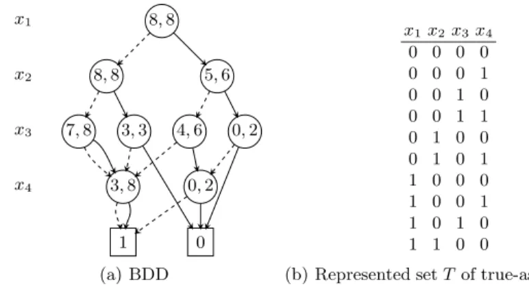
Fig. 1 A threshold BDD representing the linear constraint 2x1+5x2+4x3+3x4≤8. Edges with parity 0
are dashed
We provide a short definition of BDDs as they are used in this paper. A BDD for a set of variablesx1, . . . , xd is a directed acyclic graphG=(V , A), see Fig.1a. All nodes associated with the variablexi lie on the same level labeled withxi, which means, we have an ordered BDD (OBDD). In this paper all BDDs are ordered. For the edges there is a parity function par:A→ {0,1}. The graph has one node with in-degree zero, called the root and two nodes with out-degree zero, called leaf 0 resp. leaf 1. Apart from the leaves all nodes have two outgoing edges with different parity. A pathe1, . . . , edfrom the root to one of the leaves represents a variable assignment, where the level labelxi of the starting node ofej is assigned to the value par(ej). An edge crossing a level with nodes labeledxi is called a long edge. In that case the assignment forxiis free. All paths from the root to leaf 1 represent the setT ⊆ {0,1}d of true-assignments. The size of a BDD is defined as the number of nodes|V|. Letwl be the number of nodes in levell. The width of a BDD is the maximum of all number of nodes in a levelw=max{wl|l∈1, . . . , d}.
Verticesu, v∈V with the same label are equivalent if both of their edges with the same parity point to the same node respectively. If each path from root to leaf 1 contains exactlyd edges the BDD is called complete. A complete and ordered BDD with no equivalent vertices is called a quasi-reduced ordered BDD (QOBDD). A ver-texv∈V is redundant if both outgoing edges point to the same node. If an ordered BDD does neither contain redundant nor equivalent vertices it is called reduced or-dered BDD (ROBDD). For a fixed variable ordering both QOBDD and ROBDD are canonical representations.
A BDD representing the setT = {x∈ {0,1}d: aTx≤b}of 0/1 solutions to the linear constraintaTx≤bis called a threshold BDD. For each variable ordering the size of a threshold BDD is bounded by O(d(|a1| + · · · + |ad|)), i.e. if the weights a1, . . . , adare polynomial bounded ind, the size of the BDD is polynomial bounded ind (see Wegener 2000). Hosaka et al. (1997) provided an example of an explic-itly defined threshold function for which the size of the BDD is exponential for all variable orderings.
2 Output-sensitive building of a threshold BDD
In this section we give a new output-sensitive algorithm for building a threshold QOBDD of a linear constraint aTx ≤b in dimensiond. This problem is closely related to the knapsack problem. Our algorithm can easily be transformed to work for a given equality, i.e. it can also solve the subset sum problem.
A crucial point of BDD construction algorithms is the in advance detection of equivalent nodes (Meinel and Theobald1998). If equivalent nodes are not fully de-tected this leads to isomorphic subgraphs. As the representation of QOBDDs and ROBDDs is canonical these isomorphic subgraphs will be detected and merged at a later stage which is a considerable overhead.
We now describe an algorithm that overcomes this drawback. Our detection of equivalent nodes is exact and complete so that only as many nodes will be built as the final QOBDD consists of. No nodes have to be merged later on. Letwbe the width of the BDD. The runtime of our algorithm is O(dwlog(w))
W.l.o.g. we assume∀i∈ {1, . . . , d}ai≥0 (in caseai<0 substitutexiwith 1− ¯xi). In order to exclude trivial cases letb≥0 anddi=1ai> b. For the sake of simplicity be the given variable ordering the canonical variable orderingx1, . . . , xd. We assign weights to the edges depending on their parity and level. Edges with parity 1 in levell costaland edges with parity 0 cost 0. The key to exact detection of equivalent nodes are two bounds that we introduce for each node, a lower boundlband an upper bound ub. They describe the interval[lb, ub]. Letcube the costs of the path from the root to the node u. All nodesuin levell for which the valueb−cu lies in the interval [lbv, ubv]of a nodevin levellare guaranteed to be equivalent with the nodev. We call the value b−cu the slack. Figure1a illustrates a threshold QOBDD with the interval bounds set in each node.
Algorithm 1 Build QOBDD for the constraintaTx≤b BUILDQOBDD(slack, level)
1: if slack<0 then 2: return leaf 0
3: if slack≥di=levelaithen 4: return leaf 1
5: if exists nodevin level withlbv≤slack≤ubvthen 6: returnv
7: build new nodeuin level 8: l=level of node
9: 0-edge son=BUILDQOBDD(slack,l+1) 10: 1-edge son=BUILDQOBDD(slack-al,l+1) 11: set lb to max(lb of 0-edge son,lb of 1-edge son+al) 12: set ub to min(ub of 0-edge son,ub of 1-edge son+al) 13: returnu
Algorithm1constructs the QOBDD top-down from a given node in a depth-first-search manner. We set the bounds for the leaves as follows:lbleaf 0= −∞,ubleaf 0=
−1,lbleaf 1=0 andubleaf 1= ∞. We start at the root with its slack set tob. While traversing downwards along an edge in step 9 and 10 we substract its costs. The sons of a node are built recursively. The slack always reflects the value of the right hand sideb minus the costscof the path from the root to the node. In step 5 a node is detected to be equivalent with an already built node vin that level if there exists a nodevwith slack∈ [lbv, ubv].
If both sons of a node have been built recursively at step 11 the lower bound is set to the costs of the longest path from the node to leaf 1. In case one of the sons is a long edge pointing from this levellto leaf 1 the valuelbleaf 1 has to be temporarly increased bydi=l+1ai before. In step 12 the upper bound is set to the costs of the shortest path from the node to leaf 0 minus 1. For this reason the interval [lb, ub] reflects the widest possible interval for equivalent nodes.
Lemma 1 The detection of equivalent nodes in Algorithm1is exact and complete. Proof Assume to the contrary that in step 7 a new nodeuis built which is equivalent to an existing nodevin the level. Again letcu be the costs of the path from the root to the nodeu. Because of step 5 we haveb−cu ∈ [lbv, ubv].
Caseb−cu< lbv: In step 11 lbv has been computed as the costs of the longest path from the node v to leaf 1. Let lbu be the costs of the longest path from nodeuto leaf 1. Then there is a path from root to leaf 1 using nodeuwith costs cu+lbu≤b, so we havelbu< lbv. As the nodesuandvare equivalent they are the root of isomorphic subtrees, and thuslbu=lbvholds.
Caseb−cu> ubv: With step 12ubvis the costs of the shortest path fromvto leaf 0 minus 1. Letubube the costs of the shortest path fromuto leaf 0 minus 1. Again the nodesuandvare equivalent so for both costs we haveubu=ubv. Thus there is a path from root to leaf 0 using nodeuwith costscu+ubu< b which is a
contradiction.
Algorithm1can be modified to work for a given equality, i.e. it can also be used to solve the subset sum problem. The following replacements have to be made: 1: replace slack<0 with slack<0∨slack>di=levelai,
3: replace slack≥di=levelai with slack=0∧slack=
d i=levelai.
3 Parallel AND operation on threshold BDDs
Given a set of inequalitiesAx≤b,A∈Zm×d,b∈Zm, we want to build the ROBDD representing all 0/1 points satisfying the system. This problem is closely related to the multidimensional knapsack problem. Our approach is the following. For each of themlinear constraintsaTi x≤bi we build the QOBDD with the method described in Sect.2. Then we build the final ROBDD by performing an AND operation on all QOBDDs in parallel. The space consumption for saving the nodes is exactly the num-ber of nodes that the final ROBDD consists of plusdtemporary nodes. Algorithm2 describes our parallel and-synthesis ofmQOBDDs.
Algorithm 2 Parallel conjunction of the QOBDDsG1, . . . , Gm PARALLELANDBDDS(G1, . . . , Gm) 1: if∀i∈ {1, . . . , m} :i=leaf 1 then 2: return leaf 1 3: if∃i∈ {1, . . . , m} : i=leaf 0 then 4: return leaf 0
5: if signature(G1, . . . , Gm)∈ComputedTable then 6: return ComputedTable[signature(G1, . . . , Gm)] 7: xi=NEXTVARIABLE(G1, . . . , Gm)
8: 0-edge son=PARALLELANDBDDS(G1|xi=0, . . . , Gm|xi=0)
9: 1-edge son=PARALLELANDBDDS(G1|xi=1, . . . , Gm|xi=1)
10: if 0-edge son=1-edge son then 11: return 0-edge son
12: if∃nodevin this level with same sons then 13: returnv
14: build nodeuwith 0-edge and 1-edge son 15: ComputedTable[signature(G1, . . . , Gm)] =u 16: returnu
We start at the root of all QOBDDs and construct the ROBDD from its root top-down in a depth-first-search manner. In steps 1 and 3 we check in parallel for trivial cases. Next we generate a signature for this temporary node of the ROBDD in step 5. This signature is a 1+mdimensional vector consisting of the current level and the upper bounds saved in all current nodes of the QOBDDs. If there already exists a node in the ROBDD with the same signature we have found an equivalent node and return it. Otherwise we start building boths sons recursively from this temporary node in steps 8 and 9. From all starting nodes in the QOBDDs we traverse the edges with the same parity in parallel.
When both sons of a temporary node in the ROBDD were built we check its re-dundancy in step 10. In step 12 we search for an already existing node in the current level which is equivalent to the temporary node. If neither is the case we build this node in the ROBDD and save its signature.
In practice the main problem of the parallel and-operation is the low hitrate of the ComputedTable. This is because equivalent nodes of the ROBDD can have different signatures and thus are not detected in step 5. In addition the space consumption for the ComputedTable is enormous and one is usually interested in restricting it. The space available for saving the signatures in the ComputedTable can be changed dy-namically. This controls the runtime in the following way. The more space is granted for the ComputedTable the more likely equivalent nodes will be detected in advance which decreases the runtime. Note that because of the check for equivalence in step 12 the correctness of the algorithm does not depend on the use of the ComputedTable. If the use of the ComputedTable is little the algorithm naturally tends to exponential runtime.
Fig. 2 Dynamic programming
table for the linear constraint 2x1+5x2+4x3+3x4≤8.
VariablesUln, Dlnare shown as •,resp. The light grey blocks represent the nodes in the ROBDD and the dark grey
blocks represent the redundant
nodes in the QOBDD
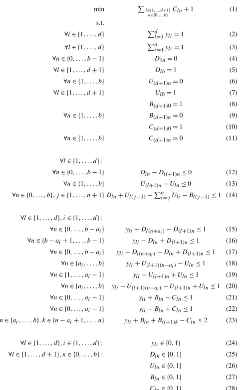
4 Optimal variable ordering of a threshold BDD via 0/1 IP formulation
Given a linear constraintaTx≤bin dimensiondwe want to find an optimal variable ordering for building the threshold ROBDD. A variable ordering is called optimal if it belongs to those variable orderings for which the size of the ROBDD is minimal. In the following we will derive a 0/1 integer program whose solution gives the optimal variable ordering and the number of minimal nodes needed.
Building a threshold BDD is closely related to solving a knapsack problem. A knapsack problem can be solved with dynamic programming (Schrijver1986) us-ing a table. We mimic this approach on a virtual table of size(d+1)×(b+1)which we fill with variables. Figure2shows an example of such a table for a fixed variable ordering. The corresponding BDD is shown in Fig.1a.
W.l.o.g. we assume∀i∈ {1, . . . , d}ai≥0, and to exclude trivial cases,b≥0 and
d
i=1ai> b. Now we start setting up the 0/1 IP shown in Fig.3. The 0/1 variables yli (24) encode a variable ordering in the way thatyli=1 iff the variablexi lies on levell. To ensure a correct encoding of a variable ordering we need that each index is on exactly one level (2) and that on each level there is exactly one index (3).
We simulate a down operation in the dynamic programming table with the 0/1 variables Dln (25). The variable Dln is 1 iff there exists a path from the root to the levell such thatb minus the costs of the path equalsn. The variables in the first row (4) and the right column (5) are fixed. We have to set variableD(l+1)nto 1 if we followed the 0-edge starting fromDln=1
Dln=1→D(l+1)n=1 (12)
or according to the variable ordering given by theyli variables, if we followed the 1-edge starting fromDl(n+ai)=1
yli=1∧Dl(n+ai)=1→D(l+1)n=1 (15)
In all other cases we have to preventD(l+1)nfrom being set to 1 yli=1∧Dln=0→D(l+1)n=0 (16) yli=1∧Dl(n+ai)=0∧Dln=0→D(l+1)n=0 (17)
In the same way, the up operation is represented by the 0/1 variablesUln (26). The variableUlnis 1 iff there exists a path upwards from the leaf 1 to the levellwith
min l∈{1,...,d+1} n∈{0,...,b} Cln+1 (1) s.t. ∀i∈ {1, . . . , d} dl=1yli=1 (2) ∀l∈ {1, . . . , d} di=1yli=1 (3) ∀n∈ {0, . . . , b−1} D1n=0 (4) ∀l∈ {1, . . . , d+1} Dlb=1 (5) ∀n∈ {1, . . . , b} U(d+1)n=0 (6) ∀l∈ {1, . . . , d+1} Ul0=1 (7) B(d+1)0=1 (8) ∀n∈ {1, . . . , b} B(d+1)n=0 (9) C(d+1)0=1 (10) ∀n∈ {1, . . . , b} C(d+1)n=0 (11) ∀l∈ {1, . . . , d}: ∀n∈ {0, . . . , b−1} Dln−D(l+1)n≤0 (12) ∀n∈ {1, . . . , b} U(l+1)n−Uln≤0 (13) ∀n∈ {0, . . . , b}, j∈ {1, . . . , n+1}Dln+Ul(j−1)− n i=jUli−Bl(j−1)≤1 (14) ∀l∈ {1, . . . , d}, i∈ {1, . . . , d}: ∀n∈ {0, . . . , b−ai} yli+Dl(n+ai)−D(l+1)n≤1 (15) ∀n∈ {b−ai+1, . . . , b−1} yli−Dln+D(l+1)n≤1 (16) ∀n∈ {0, . . . , b−ai} yli−Dl(n+ai)−Dln+D(l+1)n≤1 (17) ∀n∈ {ai, . . . , b} yli+U(l+1)(n−ai)−Uln≤1 (18) ∀n∈ {1, . . . , ai−1} yli−U(l+1)n+Uln≤1 (19) ∀n∈ {ai, . . . , b} yli−U(l+1)(n−ai)−U(l+1)n+Uln≤1 (20) ∀n∈ {0, . . . , ai−1} yli+Bln−Cln≤1 (21) ∀n∈ {0, . . . , ai−1} yli−Bln+Cln≤1 (22) ∀n∈ {ai, . . . , b}, k∈ {n−ai+1, . . . , n} yli+Bln+B(l+1)k−Cln≤2 (23) ∀l∈ {1, . . . , d}, i∈ {1, . . . , d}: yli∈ {0,1} (24) ∀l∈ {1, . . . , d+1}, n∈ {0, . . . , b}: Dln∈ {0,1} (25) Uln∈ {0,1} (26) Bln∈ {0,1} (27) Cln∈ {0,1} (28)
Fig. 3 0/1 integer program for finding the optimal variable ordering of a threshold BDD for a linear
costsn. The variables in the last row (6) and the left column (7) are fixed. We have to setUln=1 if there is a 0-edge ending inU(l+1)n=1
U(l+1)n=1→Uln=1 (13)
or according to the variable ordering given by theyli variables, if there is a 1-edge ending inU(l+1)(n−ai)=1
yli=1∧U(l+1)(n−ai)=1→Uln=1 (18)
In all other cases we have to preventUlnfrom being set to 1
yli=1∧U(l+1)n=0→Uln=0 (19) yli=1∧U(l+1)(n−ai)=0∧U(l+1)n=0→Uln=0 (20)
Next we introduce the 0/1 variables Bln (27) which mark the beginning of the blocks in the dynamic programming table that correspond to the nodes in the QOBDD. These blocks can be identified as follows: start from a variableDlnset to 1 and look to the left until a variableUlnset to 1 is found
Dln=1∧Ul(j−1)=1∧ n
i=j
Uli=0→Bl(j−1)=1 (14)
We set the last row explicitly (8,9).
At last we introduce the 0/1 variablesCln(28) which indicate the beginning of the blocks that correspond to the nodes in the ROBDD. The variablesClnonly depend on theBlnvariables and exclude redundant nodes. The first blocks are never redundant
yli=1→Bln=Cln (21,22)
If the 0-edge leads to a different block than the 1-edge, the block is not redundant
yli=1∧Bln=1∧ ⎛ ⎝ n k=n−ai+1 B(l+1)k=1 ⎞ ⎠→Cln=1 (23) We set the last row explicitly (10,11).
The objective function (1) is to minimize the number of variablesClnset to 1 plus an offset of 1 for counting the leaf 0. An optimal solution to the IP then gives the minimal number of nodes needed for the ROBDD while theylivariables encode the best variable ordering.
In practice solving this 0/1 IP is not faster than exact BDD minimization algo-rithms which are based on Friedman and Supowit’s method (Friedman and Supowit 1987) in combination with branch & bound (see Ebendt et al.2003for an overview). Nevertheless it is of theoretical interest as the presented 0/1 IP formulation can be used for the computation of the variable ordering spectrum of a threshold func-tion. The variable ordering spectrum of a linear constraintaTx≤b is the function
spaTx≤b: N→N, where spaTx≤b(k) is the number of variable orderings leading
to a ROBDD for the threshold function aTx≤b of size k. In order to compute spaTx≤b(k)we equate the objective function (1) withkand add it as the constraint
l∈{1,...,d+1} n∈{0,...,b}
Cln+1=kto the formulation given in Fig.3. The number of 0/1 vertices of the polytope corresponding to this formulation then equalsspaTx≤b(k). In (Behle
and Eisenbrand2007) we provide a method for counting these 0/1 vertices.
5 Computational results
We developed the toolazove 2.0which implements the output-sensitive build-ing of QOBDDs and the parallel AND synthesis as described in Sects. 2 and 3. It can be downloaded from (Behle 2007). In contrast to version 1.1 which uses
CUDD 2.4.1 (Somenzi 2005) as BDD manager, the new version 2.0 does not
need an external library for managing BDDs.
In the following we compareazove 2.0toazove 1.1which sequentially uses a pairwise AND operation (Behle and Eisenbrand2007). We restrict our com-parison to these two tools since we are not aware of another software tool specialized in counting 0/1 solutions for general type of problems. The main space consumption ofazove 2.0is due to the storage of the signatures of the ROBDD nodes. We re-strict the number of stored signatures to a fixed number. In case more signatures need to be stored we start overwriting them from the beginning.
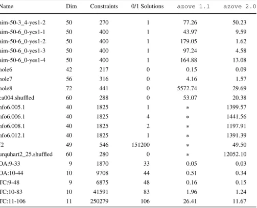
Our benchmark set contains different classes of combinatorial optimization prob-lems. All tests were run on a Linux system with kernel 2.6.15 and gcc 3.3.5 on a 64 bit AMD Opteron CPU with 2.4 GHz and 4 GB memory. Table1shows the com-parison of the runtimes in seconds. We set a time limit of 4 hours. An asterisk marks the exceedance of the time limit.
In fields like verification and real-time systems specification counting the solutions of SAT instances has many applications. From several SAT competitions (Buro and Büning1993; Hoos and Stützle 2000) we took the instances aim, hole, ca004 and hfo6, converted them to linear constraint sets and counted their satisfying solutions. The aim instances are 3-SAT instances and the hole instances encode the pigeonhole principle. There are 20 satisfiable hfo6 instances for which the results are similar. For convenience we only show the first 4 of them.
Counting the number of matchings in a graph is one of the most prominent count-ing problems with applications in physics in the field of statistical mechanics. We counted the number of matchings for the urquhart instance, which comes from a par-ticular family of bipartite graphs (Urquhart 1987), and for f2, which is a bipartite graph encoding a projective plane known as the Fano plane.
The two instance classes OA and TC were taken from a collection of 0/1 polytopes that has been compiled in connection with (Ziegler1995). Starting from the convex hull of these polytopes as input we counted their 0/1 vertices.
For instances with a large number of constraintsazove 2.0clearly outperforms version 1.1. Due to the explosion in size during the sequential AND operation azove 1.1is not able to solve some instances within the given time limit. The parallel AND operation inazove 2.0successfully overcomes this problem.
Table 1 Comparison of the toolsazove 1.1andazove 2.0
Name Dim Constraints 0/1 Solutions azove 1.1 azove 2.0
aim-50-3_4-yes1-2 50 270 1 77.26 50.23 aim-50-6_0-yes1-1 50 400 1 43.97 9.59 aim-50-6_0-yes1-2 50 400 1 179.05 1.62 aim-50-6_0-yes1-3 50 400 1 97.24 4.58 aim-50-6_0-yes1-4 50 400 1 164.88 13.08 hole6 42 217 0 0.15 0.09 hole7 56 316 0 4.16 1.57 hole8 72 441 0 5572.74 29.69 ca004.shuffled 60 288 0 53.07 20.38 hfo6.005.1 40 1825 1 ∗ 1399.57 hfo6.006.1 40 1825 4 ∗ 1441.56 hfo6.008.1 40 1825 2 ∗ 1197.91 hfo6.012.1 40 1825 1 ∗ 1391.39 f2 49 546 151200 ∗ 49.50 urquhart2_25.shuffled 60 280 0 ∗ 12052.10 OA:9-33 9 1870 33 0.05 0.03 OA:10-44 10 9708 44 0.51 0.34 TC:9-48 9 6875 48 0.16 0.15 TC:10-83 10 41591 83 1.96 1.24 TC:11-106 11 250279 106 26.41 11.67 References
Becker B, Behle M, Eisenbrand F, Wimmer R (2005) BDDs in a branch and cut framework. In: Nikolet-seas S (ed) Proceedings of the 4th international workshop on efficient and experimental algorithms (WEA’05). Lecture notes in computer science, vol 3503. Springer, Berlin, pp 452–463
Behle M (2007) Another zero one vertex enumeration tool homepage.http://www.mpi-inf.mpg.de/~behle/ azove.html
Behle M, Eisenbrand F (2007) 0/1 vertex and facet enumeration with BDDs. In: Applegate D, Brodal GS, Panario D, Sedgewick R (eds) Proceedings of the 9th workshop on algorithm engineering and experiments (ALENEX’07). SIAM, Philadelphia, pp 158–165
Bollig B, Wegener I (1996) Improving the variable ordering of OBDDs is NP-complete. IEEE Trans Com-put 45(9):993–1002
Bryant RE (1986) Graph-based algorithms for Boolean function manipulation. IEEE Trans Comput 35:677–691
Buro M, Büning HK (1993) Report on a SAT competition. Bull Eur Assoc Theor Comput Sci 49:143–151 Ebendt R, Günther W, Drechsler R (2003) An improved branch and bound algorithm for exact BDD
minimization. IEEE Trans Comput-Aided Des Integr Circuits Syst 22(12):1657–1663
Friedman S, Supowit K (1987) Finding the optimal variable ordering for binary decision diagrams. In: Pro-ceedings of the 24th ACM/IEEE design automation conference. IEEE Computer Society Press/ACM, Los Alamitos/New York, pp 348–356
Hoos HH, Stützle T (2000) SATLIB: An online resource for research on SAT. In: Gent IP, Walsh T (eds) Satisfiability in the year 2000. IOS Press, Amsterdam, pp 283–292
Hosaka K, Takenaga Y, Kaneda T, Yajima S (1997) Size of ordered binary decision diagrams representing threshold functions. Theor Comput Sci 180:47–60
Lee CY (1959) Representation of switching circuits by binary-decision programs. Bell Syst Tech J 38:985–999
Meinel C, Theobald T (1998) Algorithms and data structures in VLSI design. Springer, New York Schrijver A (1986) Theory of linear and integer programming. Wiley, New York
Somenzi F (2005). CU decision diagram package release 2.4.1 homepage. Department of Electrical and Computer Engineering, University of Colorado at Boulder.http://vlsi.colorado.edu/~fabio/CUDD
May 2005
Urquhart A (1987) Hard examples for resolution. J ACM 34(1):209–219
Wegener I (2000) Branching programs and binary decision diagrams. SIAM monographs on discrete math-ematics and applications. SIAM, Philadelphia