Identifying residential water end-uses underpinning peak day and peak
hour demand
Authors:
Cara D. Beal1 (corresponding author)
1
Research Fellow, Smart Water Research Centre, Griffith University, Gold Coast Campus, 4222 Australia, E-mail: c.beal@griffith.edu.au
Rodney A. Stewart2
3
Director, Centre for Infrastructure Engineering & Management, Griffith University, Gold Coast Campus, 4222, Australia, E-mail: r.stewart@griffith.edu.au
Citation: Beal, C.D., Stewart, R.A., (2013). "Identifying Residential Water End-Uses Underpinning Peak Day and Peak Hour Demand." J. Water Resour. Plann. Manage., doi: 10.1061/(ASCE)WR.1943-5452.000035.
Abstract
Accurate and up-to-date peak demand data is essential to ensure that future mains water supply networks reflect current usage patterns and are designed efficiently from an engineering, environmental and economic perspective. The aim of this paper was to identify the water end-uses which drive peak day demand and to examine their associated hourly diurnal demand patterns based on over 18 months of water consumption data obtained from high resolution smart meters installed in 230 residential properties across south east Queensland, Australia. Peak Day (PD) to Average Day (AD) ratios between 1-1.5 were driven by both external and internal end-uses. However, as the PD:AD ratio increased above 1.5, demand was driven largely by external water usage (i.e. lawn and garden irrigation).. Peak hour ratios (i.e. PHPD:PHAD) ranged from 1.3 to 3.0 for the four peak demand days. At the end-use level, the individual end-use category PHPD:PHAD ratios were in the range of 0.7 – 3.3 for all end-uses, with the exception of external or irrigation. The ratio for this latter end-use category was typically very high, at over 10 times the average irrigation demand. Comparisons with historically-based, but currently used, peaking factors used for network distribution modelling suggests that the degree and frequency of high peaking factors are lower now, due to the high penetration of water-efficient technology and growing water conservation awareness by consumers.
Keywords: water end-use consumption, water micro-components, water demand management, peak demand, urban water supply design
Introduction
Urban water planning and design
A reticulated water supply is considered one of the most significant infrastructure assets in a community (Savic and Walters 1997), and as such, the optimal planning and design of this infrastructure is critical. It has been recognised that urban network planning needs to be more optimised (Lucas et al. 2010), and in this regard, understanding the patterns of residential water demand is paramount. Residential water consumption patterns typically vary on both a daily basis, where an average day peak hour demand will occur, and on an annual basis, where a peak day demand will occur. Moreover, there is an annual peak hour demand that can be many multiples of the average day peak hour consumption. Previous research demonstrates that variations in consumption are mainly driven by climate (rainfall and temperature), household demand, consumer behaviour, household stock water efficiency and consumer socio-demographics (Beal and Stewart 2011, Willis et al. 2011a, Arbues et al. 2010). Key water design planning parameters for construction of water delivery infrastructure are the average day, peak day and peak hour demand (Swamee and Sharma 2008, Lucas et al. 2010). Peaking factors are calculated from the average and peak day demand values including the peak day factor which is the ratio of peak day demand/average day demand (PD/AD). A range of peaking factors reported in the literature, is presented in Table 1.
Understanding peaking factors are critical in determining the pipe infrastructure that is sufficient to deliver water during peak water demand periods. Numerous models and algorithms have been developed over several decades which have required the fundamental input parameter of peak hour demand (Goulter and Morgan 1985, Savic and Walters 1997, Jacobs 2007, Adamowski and Karapataki 2010, Alcocer-Yamanaka et al. 2012); these are typically based on top-down estimations rather than bottom-up actual measurement. Also,
beyond the strict engineering focus, AD and PD data and diurnal demand patterns are vital empirical input parameters for other decision support tools for integrated urban water planning such as those proposed by Lim et al. (2010) and Makropoulos et al. (2008).
Table 1. Peaking factor ranges reported in the literature
Peaking factor range Location Source
Peak day
1.0 to 1.5 Data used from various cities in
South Africa, France, USA
Van Zyl et al. (2008, 2011)
1.1 to 1.7 North West England, UK Surendran et al. (2005)
1.4 to 2.0 Ireland Twort et al. (1994)
1.5 to 2.0 Victoria, Australia WSAA (2002)
1.5 to 2.3 Queensland, Australia DERM (2010)
1.8 to 2.9 Various cities, UK Twort et al. (1994)
Peak hour
1.0 to 1.5 Data used from various cities in
South Africa, France, USA
Van Zyl et al (2008, 2011)
1.2 to 1.8 Boston, USA Shvartser et al. (1993)
2 to 5 Various cities, Australia WSAA (2002)
3.6 to 5.0 Queensland, Australia DERM (2010)
In recent times, through either a mandatory or voluntary basis, new developments have incorporated a much higher degree of water-efficient stock than previously (e.g. low water use clothes washers, toilets and shower fittings) (Beal et al. 2011, Polebitski et al. 2011). Additionally, these new developments commonly adopt alternative water sources such as rainwater tanks (Lucas et al. 2010, Willis et al. 2011a). Therefore, on balance, water
consumption parameters (volume and frequency of use) today are likely to be considerably different to 20, 10 or even 5 years ago due to the presence of technology designed to reduce mains water flow. Accurate and up-to-date peak demand data is therefore essential to ensure that future mains water supply (and sewerage) networks reflect current usage patterns and are designed efficiently from an engineering, environmental and economic perspective.
Using disaggregated water consumption data to identify peak demand
Water end-use studies (also known as water micro-component studies) provide a fundamental basis for evaluating the effectiveness of a range of water demand management strategies. End-use studies also inform water demand modelling forecasts which underpin all water service infrastructure modelling and reticulation plans (Jacobs, 2007; Blokker et al. 2010). Knowledge of the average and peak end-use water consumption volumes (e.g. toilet, tap, shower, clothes washer, external [e.g. irrigation] and leaks) at hourly, daily and monthly levels of resolution, can strongly inform the planning process (Mayer et al. 2006; Beal et al. 2011; Willis et al. 2011b).
Diurnal water end usage patterns can also be generated from high resolution micro-component data. Diurnal usage patterns have been used to identify trends and peaks in water (e.g. Willis et al. 2011a) and energy (e.g. Firth et al. 2008) consumption over time Stewart et al. (2010) also noted that this type of peak demand analysis can provide valuable information to water utilities to address issues such as planning, asset management and hydraulic engineering based problems.
These patterns have aided in the characterisation of daily water consumption trends across different socio-demographic groups and varying climatic regions (Beal et al. 2011; Willis et al. 2011b). Diurnal patterns provide valuable information on demand (per capita) and end-use
consumption at an hourly level for AD demand in a study period. Other benefits of such data include the real-time observation of AD peaks and troughs, understanding daily demand quantities and reservoir storage needs as well as creating demand parameters for optimisation of the supply infrastructure through offsets to network upgrades (Beal et al. 2010; Basupi et al. 2011; Stewart et al. 2010). Diurnal water end-use patterns can also be examined for peak day demand, allowing a greater understanding of the types of household practices that drive peak usage.
Drawing from the identified research gaps and the clear need for a greater understanding of peak flows in new developments, the objectives of this study are to:
1. identify the water end-uses which drive peak demand using measured water end-use data;.
2. determine the peak day diurnal demand patterns at an end-use level of resolution; 3. determine the relative frequency of peaking factors over the study period of
measurement;
4. determine ratios of peak to average day demand, and average day peak hour with peak day peak hour demand and compare with ratios reported in the literature; and
5. provide recommendations on how high resolution smart water metering and end-use studies can enable improved future urban water infrastructure planning.
Methodology
The data for the current study was generated from the South East Queensland Residential End-use Study (SEQREUS) located in the south eastern corner of Queensland, Australia (Beal and Stewart 2011). The methodological approach used to obtain the data for this paper is shown in Fig. 1.
Fig. 1. Process used for obtaining water end-use data on selected peak demand days.
Study sample characteristics
A total of 230 households were used in this study, providing a good representation of SEQ households with a varying range of household occupancies, family composition and household income categories (Table 2). The rainfall and temperature data for the three periods of measurement are provided in Table 3. Of note, the summer 2010-11 recorded above average rainfall with widespread flooding throughout SEQ. This substantially reduced the need for irrigation over the summer period, and also resulted in a considerable number of the data loggers malfunctioning, due to water ingress.
Table 2. Selected characteristics of households in the SEQREUS sample
Sample Characteristics1 Gold
Coast Brisbane Ipswich
Sunshine Coast SEQ combined Household occupancy 2.6 2.6 2.7 2.5 2.6 No of people 230 164 96 171 661 No. homes 65 61 37 67 230
% Households with ≤ 2 people 58 41 51 69 55
% Households
pensioners/retired 36 16 32 45 32
% Households with children
(aged ≤ 17) 34 30 21 25 28
Average age of children
(years) 8.8 2.7 4.4 10 6.5
Average household income
($AUD)2 73,290 81,630 87,900 60,070 75,722
Notes: 1data presented are averages; 2Estimated from taking the average of the household income category that each respondents selected (Gregory and Di Leo 2003), where categories were: 1 = <$30,000, 2 = $30,000 – $59,000, 3 = $60,000 – $89,999, 4 = $90,000 - $119,999, 5 = $120,000 - $149,999, 6 ≥ $150,000.
Table 3. Climate data for four regions during the specific periods of flow trace analysis1 Study
region
Average Maximum (°C) Total rainfall (mm) No. of wet days2
Winter 2010 Summer 10-11 Winter 2011 Winter 2010 Summer 10-11 Winter 2011 Winter 2010 Summer 10-11 Winter 2011 Gold Coast3 21.3 (±0.8) 27.9 (±1.7) 20.5 (±2.9) 21.5 567.2 20.4 4 25 4 Brisbane4 21.4 (±0.9) 27.9 (±1.7) 20.1 (±3.5) 9.6 488.7 6.5 2 29 2 Ipswich5 21.8 (±1.2) 28.7 (±2.9) 20.3 (±3.7) 8.8 342.2 9.2 1 22 2 Sunshine Coast6 21.4 (±0.9) 27.6 (±1.6) 21.3 (±3) 47.1 543.7 8.6 7 27 1
Notes: 1 Data taken from Bureau of Meteorology (BOM) http://www.bom.gov.au/climate/data/index.shtml; 2 Number of days where rainfall ≥1mm; 3 average of Coolangatta and Gold Coast BOM stations; 4 average of Brisbane Airport and Archerfield BOM stations; 5 Amberley BOM station; 6 average of Sunshine Coast airport and Tewantin BOM stations, 7 (±x) indicates standard deviation from mean for the period of analysis.
Disaggregating total flow into individual end-uses
The SEQREUS, on which the data for this paper is based, used a mixed method, advanced water end-use measurement approach to capture and analyse water use data (Fig. 2). Full details of the methods used to undertake these measurements is provided in Beal and Stewart (2011), however a short summary is provided here.
Upon completion of recruitment, standard council residential water meters were replaced with modified Actaris CTS-5 water meters. These ‘smart’ meters measure flow to a resolution of 72 pulses/L or a pulse every 0.014 L. The smart meters were connected to Aegis Data Cell series R-CZ21002 data loggers. The loggers were programmed to record pulse counts at five second intervals. This data was wirelessly transferred to a central computer, via email, and stored in a database for subsequent analysis
Fig. 2. Mixed method approach used in the SEQREUS. Inset: location of study in Qld, Australia.
A representative sample of received data was extracted from the database and disaggregated into all end-use events associated with the sampled residential households. Disaggregation of total household flow into the specific end-uses such as irrigation, toilet, clothes washer, shower and tap, was performed using the software package Trace Wizard ® (Aquacraft 2010, Mayer et al. 2006). This software allows the user to identify specific flow patterns and assign them into end-use categories, and is a commonly accepted method of disaggregating fixture/appliance events from a single flow meter (Froehlich et al. 2011). Using this flow trace analysis to disaggregate flow has shown to have over an 80% accuracy rate (Wilkes et al. 2005). This is likely to be higher for single event identification, identification of automated appliances such as clothes washers and dishwashers, and also when using a high resolution smart meter such as those employed in the current study (Mayer et al. 1999, 2006).
Flow trace and water use
analysis
Household audit of all water appliances
Self-reported water diary MAINS WATER Household water use survey Smart meter records flows of .014L/pulse Pulses logged at 5 sec. intervals and stored in data logger Data remotely transferred via email 9% 16% 26% 28% 16% 5% Leak Toilet Clothes Washer Shower Tap Irrigation X
In the current study, we have included two further steps to the normal process to further improve flow trace analysis accuracy, including a detailed water audit of household water use behaviours and water use stock efficiency as well as asking them to complete a water use diary for a week period. Both of these extra measures ensure that the analyst using the flow trace software will be able to establish robust categorisation templates and could understand user behaviours (e.g. use bath in the evening). The event flow signature and this understanding of each homes water use behaviours enabled accurate end-use disaggregation in this study.
Identification of end-uses is informed not only by the high resolution trace flows, but also the specific knowledge of each household’s fixtures and appliances. Thus, concomitantly with meter and logger installation, a water fixture/appliance stock survey was conducted at each participating home in order to investigate how householders interact with such stock (Fig. 2). By completing the stock survey, the householder provided information on the number and degree of water-efficient appliances and the typical water consumption behaviours of the householders. As discussed, this facilitated the disaggregation of trace flows from each home and also provided a valuable snapshot of the daily water consumption habits within each home.
The limitations of the software relate to the ability to discern multiple simultaneous events and low flow external consumption. These limitation can be substantially minimised by high resolution meters, experienced analysts and a comprehensive understanding of the water use stock, and habits / behaviours of the participants involved. All these factors were considered in the experimental design phase and implemented in the establishment phase of the
SEQREUS project. Further discussion on the research methods is provided in Beal and Stewart (2011).
Diurnal pattern generation and peak demand ratios
Using the SEQREUS database, a complete timeline of average daily total water consumption was sourced from 567 days of continuous logging from up to 230 homes per day, equating to over 93,000 measured data points. From this, peak demand days could be clearly seen over the timeline with four being selected for further detailed examination. The four peak days were selected as they included both week and weekend days and occurred during ‘business as usual’ and holiday (e.g. Christmas / summer holidays) periods.
AD demand was calculated by averaging the consumption from 230 homes over the 18 month measurement period. AD diurnal demand patterns, at an end-use level, were generated using a software application specifically developed for this study. The software package is a basic windows executable file (.exe) that gathers the start and completion time of each characterised end-use event from all of the respective end-use database files, and assigns the events to the respective hourly time-of-use interval (e.g. 11.00 to 12.00 am). After accumulation of the water used by each end-use in each respective hourly period of the day, the program divides by the number of days in the study period, as well as the number of people or households in the sample size depending on unit of analysis requirements. For this paper, the units were in average litres per person per hour per day (L/p/h/d). Diurnal water end-use patterns were generated from consumption data for a number of average and peak day periods.
Results and Discussion
Water end-use breakdown of peak day demand
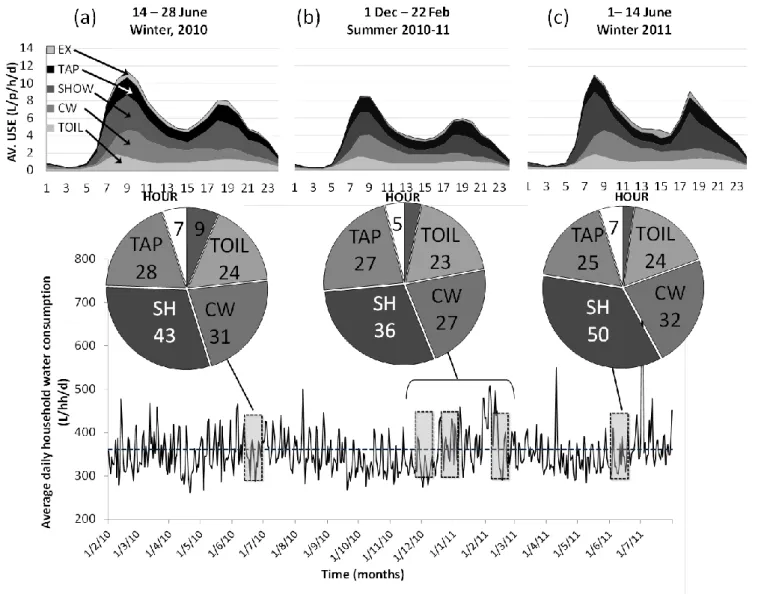
The timeline of daily total household water consumption (L/hh/d), recorded from all functioning data loggers, is presented as a combined SEQ average (Fig. 3). The Insets (a) to (d) presented in Fig. 3 provide per capita water end-use breakdowns (L/p/d) for a 24 hour period for four days of above average water consumption: Thursday, 30/12/2010 (Fig. 3a), Friday, 07/01/11 (Fig. 3b), Sunday, 10/04/2011 (Fig. 3c), and Saturday, 02/07/11 (Fig. 3d). Also shown are reproductions of the winter 2010 (Fig. 3e), summer 2010-11 (Fig. 3f) and winter 2011 (Fig. 3g) end-use pie charts (Beal and Stewart 2011). Inclusion of these pie charts offer ‘baseline’ datasets for comparison with the end-use breakdowns from peak demand days. Note that the pie charts and diurnal usage patterns for the peak demand days are generated from a smaller, random sample size (n = 25). This smaller sample size is due to the human resource requirements to undertake the Trace Wizard® analysis which generates end-use breakdowns. As such, the pie charts and diurnal usage patterns have been included to provide an indication or snapshot only of the type of end-use activities that typically contribute to peak hour and peak day demand.
The end-use consumption data for selected peak days are presented in the pie charts shown in Insets (a), (b) and (c) of Fig. 3. For comparison, the baseline data from the three SEQREUS reads, are shown in Fig. 3e-3g. Peak day water consumption is clearly higher than baseline consumption for shower (SHOW), clothes washer (CW), toilet (TOIL) and external (EX) (Fig 3a-3d). For the indoor uses of shower, clothes washer and toilet, average peak volumes are 23%, 96% and 49% greater than the baseline, respectively. For external end-uses, which are assumed to be primarily irrigation and high tap use, there is considerable variation between
the peak consumption volumes, averaged at 24 L/p/d for the four days with a standard deviation of 25.4 L/p/d.
There was little variation in tap usage across all pie chart snapshots, suggesting that this is not likely to be an end-use that would drive peak day demand, although it may be attributable to peak hour demand, if they are external tap fixtures. Note that the ‘tap’ category in this paper refers to indoor tap use or low external tap use. Large tap events have been allocated to the external water use category, as this is typically the location of such large flows from taps (Mayer and DeOreo 1999).
1 2
Notes: EX = external, TOIL = toilet, CW = clothes washer, SHOW = shower, DW = dishwasher, L = leak. 3
Fig. 3. Timeline for total water consumption showing water use breakdown in L/p/d and average daily 4
diurnal water use (L/p/h/d) for baseline data during (a) winter 2010, (b) summer 2010-11, (c) winter 2011. 5
6
Diurnal breakdown of peak demand 7
The peak hour demand for each of the four days investigated ranged from 10.8 L/p/h/d to 8
30.8 L/p/h/d (Fig. 3a-d). The uniform, twin peak periods occurring in the morning and 9
afternoon which are typically seen in average day demand diurnal patterns (Fig. 3e) are not so 10
evident for the four peak day demand diurnal patterns shown in Fig. 3a-d. The peak day 11
diurnal patterns exhibited a frequent occurrence of peak events throughout the day, 12
particularly for the external water usage. The greatest peak demand day of 605 L/hh/d (261 13
L/p/d) on 02/07/11 is shown in Inset (d) and is clearly driven by external (irrigation) water 14
use where the peak hour and peak day irrigation demand was 13.4 L/h/p/d and 140 L/hh/d (61 15
L/p/d), respectively. In terms of peak hour versus peak day consumption; large outdoor usage 16
events are more likely to primarily drive peak hour demand, relative to the overall peak day 17
demand. Whereas peak day demand may be influenced by both indoor and outdoor end-uses. 18
For example, high shower and clothes washer usage dominated total household consumption 19
as shown in the 30/12/10 and 07/01/11 pie and diurnal charts (Fig. 3a,b). Others have also 20
drawn similar conclusions on the different end-uses driving peak hour versus peak day 21
demand (Cole and Stewart 2012; Polebitski et al. 2011; Lucas et al. 2010). 22
23
One other important characteristic of the peak day diurnal patterns is the timing of the 24
external water use activities. In the State of Queensland, where the data was sourced from, 25
there is a current restriction on irrigation between 10 am and 4 pm. The results demonstrate a 26
degree of non-compliance during this timeframe and further, this practice appeared to have 27
increased rather than decreased over the 18 month monitoring period, judging by the 28
consumption timeline shown in Fig. 4. 29
31
Fig. 4. Timeline for total water consumption showing water use breakdown in L/p/d and 32
average daily diurnal water use (L/p/h/d) for the selected peak demand days of (a) 30/12/10, 33
(b) 07/01/11, (c) 10/04/11, and (d) 02/07/11. 34
Peaking factors and end-use analysis 36
The peaking factor (PF) is the ratio of the maximum flow to the average daily flow in a water 37
system.Peaking factors for peak day (e.g. PD/AD) and peak hour (e.g. PHPD/PHAD) are the 38
basis for designing mains water supply infrastructure. Pipe infrastructure must be designed 39
such that it can handle peak demand periods without a loss in pressure to the customer below 40
desired service standards. While it is acknowledged that annual AD (AAD) and PD/AAD are 41
conventionally used in infrastructure modelling, all the data (across 18 months) was used for 42
this study as the seasonal variation is less marked in the subtropical climate of Queensland, 43
with rainfall or dry periods often occurring out of the typical winter or summer periods. (Note 44
that statistical tests revealed that comparison of means of the AD and AAD datasets were not 45
significantly different [p>0.1] at 356 L/hh/d [SD±51.4] and 353.3 L/hh/d [SD±52.4], 46
respectively). 47
48
Peak day factors 49
A breakdown of average daily total water consumption showing the peaking factor trend for 50
the combined SEQ sample is shown in Fig. 5. The four peak demand days selected had 51
increasing peak day factors of 1.3, 1.5, 1.6 and 1.7 (Fig. 5). Generally, the proportion of 52
external consumption increased concomitantly with the increase in peaking factor. Less than 53
a third of the data had peaking factors over 1, suggesting extreme usage from a small number 54
of days may have a strong influence on the average peaking factor of any given region in this 55
sample. This trend also supports previous research regarding peaking factors and network 56
distribution design (e.g. Basupi et al 2011; Swamee and Sharma 2008; Savic and Walters 57
1997). The relative frequency distribution of PD/AD for each month is shown in Fig. 5b 58
(inset) where it can be observed that PD/AD factors between 0.8 and 1.2 occurred at the 59
greatest frequency. Knowledge on the range and distribution of peaking factors can inform 60
water distribution modelling, particularly if historical, and potentially out-dated factors, 61
continue to be applied. The peaking factor values reported here, determined from 18 months 62
of measured water consumption, lie within the lower end of the range reported for local 63
guidelines; of 1.5 to 2.3 (DERM, 2010), but well within the ranges reported elsewhere in the 64
literature (Table 1). This suggests that in Queensland, and particularly in urban areas in the 65
South East corner, where water consumption is trending downwards (Willis et al. 2011b, Beal 66
and Stewart 2011), there is a potential for over-sizing of water distribution infrastructure to 67
new residential developments. The reduced consumption in new dwellings in Queensland is 68
discussed in more detail later in the paper. 69
70
Fig. 5. Breakdown of (a) average daily total water consumption (LHS) and PD:AD ratio 71
(RHS) and (b) frequency distributions for combined SEQ sample peaking factors. 72
73
Peak hour factors and contributing end-uses 74
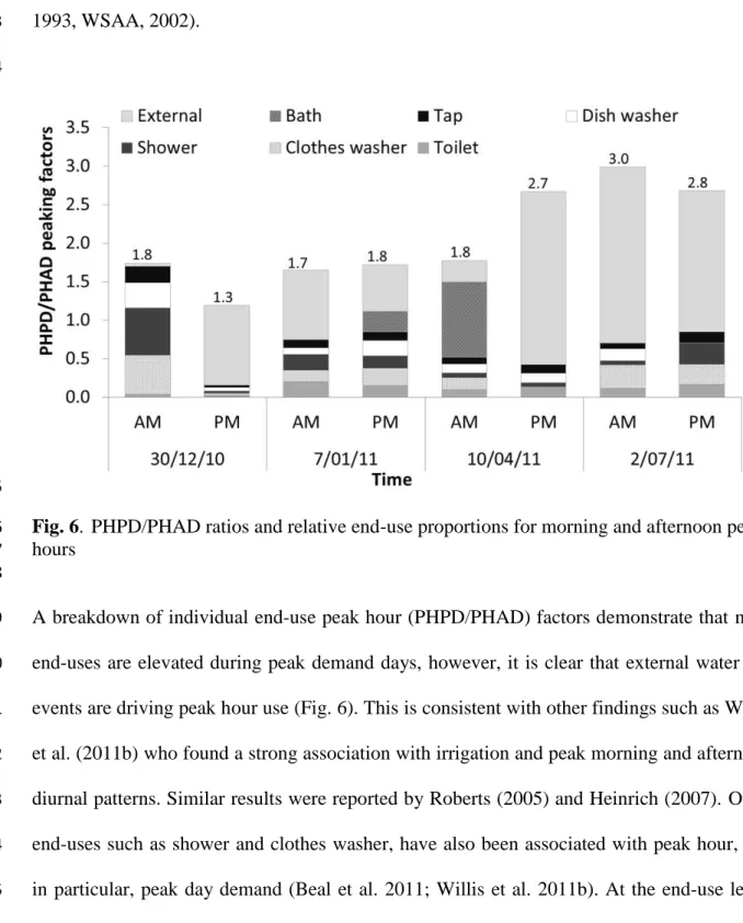
The peak hour in average day (PHAD) values (i.e. morning and evening peak hour in average 75
day) were derived from an average of the three periods of analysis: winter 2010, summer 76
2010-11 and winter 2011. The peak hour in peak day (PHPD) values were taken from each of 77
the four peak day end-use diurnal demand patterns. As expected the hourly peaking factors 78
are higher than the daily factors. Hourly peaking factors ranged from 1.7 to 3.0 in the 79
morning and 1.3 to 2.8 in the afternoon (Fig. 6). Notably, they are lower than the range of 80
Queensland government reported values (i.e. 3.6 to 5.0), although, as shown in Table 1, other 81
researchers have reported similar ranges to those observed in this study (e.g. Shvarster et al. 82
1993, WSAA, 2002). 83
84
85
Fig. 6. PHPD/PHAD ratios and relative end-use proportions for morning and afternoon peak 86
hours 87
88
A breakdown of individual end-use peak hour (PHPD/PHAD) factors demonstrate that most 89
end-uses are elevated during peak demand days, however, it is clear that external water use 90
events are driving peak hour use (Fig. 6). This is consistent with other findings such as Willis 91
et al. (2011b) who found a strong association with irrigation and peak morning and afternoon 92
diurnal patterns. Similar results were reported by Roberts (2005) and Heinrich (2007). Other 93
end-uses such as shower and clothes washer, have also been associated with peak hour, and 94
in particular, peak day demand (Beal et al. 2011; Willis et al. 2011b). At the end-use level, 95
the individual use category PHPD:PHAD ratios were in the range of 0.7 – 3.3 for all end-96
uses, with the exception of external or irrigation. The ratio for this latter end-use category 97
was typically very high, at over 10 times the average irrigation demand. 98
99
Influence of climate on total household consumption 100
A timeline of average temperature, rainfall and daily total consumption for each month of the 101
study is presented in Fig. 7. The four peak days selected for analysis are indicated by the 102
hatched triangles on the water consumption curve. There is a weak relationship between 103
increased temperature and peak demand days, although this is not consistent across the 104
timeline. There is a stronger association between temperature and total household water 105
consumption for the warmer months e.g. January to March 2010 and November to March 106
2011. Cole and Stewart (2012) report a strong correlation between temperature and bulk 107
water demand for the Hervey Bay region of Queensland, Australia. Others have also 108
observed this relationship between temperature and residential water consumption (Water 109
Corporation 2011, Willis et al. 2011b, Adamowski 2008). Another weak relationship is 110
apparent for low rainfall and increased water demand during the months of April to August 111
2010 and June to July 2011 (Fig. 7). It should be noted that the high rainfall events occurring 112
in December 2010 and January 2011 contributed to major flooding across SEQ, effectively 113
eliminating the need for irrigation during this period. 114
115
Prior to the peak per capita water usage day on 02/07/11 of 261 L/p/d (Inset (d) Fig.4), there 116
was a period of approximately four weeks where low rainfall (0.4 mm) and relative humidity 117
(59%) occurred in the SEQ region. These conditions are typical of winter climate in SEQ and 118
it is believed that the conditions were likely to have contributed to the observed sudden 119
increase in the number of irrigation events occurring on that Saturday. 120
121 122
Note: Climate data sourced from the Bureau of Meteorology http://www.bom.gov.au/climate/data/index.shtml.using data
123
averaged from the Gold Coast, Brisbane, Sunshine Coast and Ipswich weather stations – see notes from Table 3.
124 125
Fig. 7. Timeline of average monthly climate data and daily household water consumption 126
127
There is wide acknowledgement of the need to adapt to, as well as mitigate for, climate 128
change impacts on the urban water systems (Gleick 2003, Polebitski et al. 2011, Short et al. 129
2012). Recent climate modelling in Queensland has predicted shorter, but more intense, 130
rainfall patterns in the summer, resulting in longer periods of dry weather over the winter 131
months (Queensland Government 2012). Direct impacts to urban water supplies from climate 132
change, such as changes to rainfall and temperature patterns, may see the past peak water 133
usage period, historically in the hotter months (December to February) in sub-tropical 134
Queensland, shift toward the drier, cooler months in winter and spring (June to September). 135
Indeed, the data presented in this paper demonstrates that peak demand times were not 136
restricted to summer months, but instead they occurred throughout the year, in the drier 137
months of April and July. 138
139 140
Future trends in peak demand 141
There exists a strong possibility in Queensland, and indeed elsewhere in Australia, that a 142
downward trend in future peak demand will be observed. Factors influencing this downward 143
trend include the introduction of resource-efficient planning initiatives, the penetration of 144
water efficient or alternative water supply technology, and changes in consumer behaviour .. 145
146
The introduction of resource-efficient planning initiatives such as water conservation and 147
intervention programmes, high density, low footprint housing, water-efficient fixtures, 148
internally connected rainwater tanks have shown to substantially reduce household water 149
consumption (Fidar et al. 2010, Beal et al. 2012, Fielding et al. 2012). For example in SEQ, 150
average water consumption was effectively halved from 300 L/p/d to around 150 L/p/d 151
within less than 5 years (Traves et al. 2008, Walton and Hume 2011), as a result of a range of 152
water demand management approaches. Thus, this marked reduction in average consumption 153
is likely to be mirrored by a reduction in peaking factors. 154
155
The effect of water efficient technology on daily diurnal patterns and peak flow is discussed 156
by Carragher et al. (2012). They concluded that water efficient stock (e.g. low flow shower 157
roses, water-efficient clothes washers) has a significant reduction in ADPH demand and that 158
this trend towards lower peak hour consumption, will continue as new dwellings are 159
constructed, and existing homes are refurbished. Reduced peak day and peak hour demand, 160
due to residential water stock efficiency measures (including government rebate programs for 161
water-efficient appliances and water conservation awareness campaigns), has implications for 162
optimising pipe network modelling and capital infrastructure, e.g. deferral or reduction in 163
water distribution infrastructure (Basupi et al. 2011; Carragher et al. 2012). For example, 164
Tsang (2010) utilised the SEQREUS diurnal demand patterns as input into pipe network 165
models in Gold Coast City, Australia, and discovered that reduced hourly demand provided 166
spare capacity in existing pipe infrastructure, thereby reducing the need for costly 167
augmentations. 168
169
Irrigation has shown to be dramatically reduced in the post-drought and post water restriction 170
environment in SEQ (Walton and Hume 2010; Willis et al. 2011b; Beal et al. 2011). Further, 171
three years post-drought, the expected rebound back to higher (e.g. >200 – 300 L/p/d) 172
consumption is still not fully evident, despite the present high water storage levels and lack of 173
water conservation social marketing programs. Together with this entrenched water 174
conservation behaviour, the residential landscape in SEQ has changed markedly over the 175
years, with new developments being built on smaller allotment sizes, with reduced garden or 176
lawn areas. This trend towards affordable, higher density developments is evident 177
internationally (e.g. Forsyth et al. 2010). Planning guidelines in Australia also strongly 178
promote native species to be planted that require a lower frequency and volume of water. 179
180
For the various the reasons described above, household water consumption in SEQ and 181
potentially other regions internationally, is not likely to return to the daily capita usage of 300 182
L/p/d that was typical a decade ago. Consequently, the variation and volume of peak demand 183
is also likely to change (decline). It is postulated that peak demand days will not occur to a 184
lesser degree and with lower incidences of high peaking factors in the future. Some evidence 185
of this has been presented herein with lower daily and hourly peaking factors than historically 186
reported however, further analysis of the correlation between climate pattern and peak end 187
usage, based on an additional year of end-use data, is an important next step of this research. 188
189 190
Conclusions
191The aim of this study was to determine peak hourly and daily demand for a range of water 192
end-uses in households located in South East Queensland, Australia. Peak day and peak hour 193
demand was examined for four peak days identified from 18 months of empirical household 194
water consumption data. Given the reduced dominating role of irrigation contributing towards 195
peak demand in this study, other end-uses have become evident as potential contributors to 196
the lower peaking levels. Peak day demand that yielded peaking factors between 1 and 1.5 197
were observed to be driven by clothes washer and shower use, as well as external use. 198
However, peak hour demand was primarily driven by external water usage. 199
200
Overall, peaking factors were lower than those being used in current local planning 201
guidelines for residential water supply. A reduction in the degree and frequency of peak 202
demand days is likely due to the high penetration of residential water stock efficient 203
measures, water consumer behavioural changes and higher dwelling density. Thus, caution 204
should be exercised if using historic peak day and peak hour demand data for infrastructure 205
design and modelling. This is especially pertinent in jurisdictions where factors influencing 206
future water demand are evident, such as the wide incorporation of water efficient stock and 207
permanent shifts in water conservation behaviours. In these jurisdictions, future network 208
modelling and urban water system planning should carefully consider such reductions in peak 209
demand and may require the recalibration of peaking factors. 210
211
The SEQREUS has recently received additional funding to extend data collection to early 212
2015 and it is hoped that sufficient end-use data sets can be established to provide an 213
intelligent predictive tool of water end-use consumption (especially outdoor which is highly 214
variable) based on a range of variables including climatic conditions. Additionally, future 215
work will target longer time scales and a larger sub-sample of homes during peak demand 216
days, to establish greater certainty on current peaking factors and diurnal hourly patterns. 217
Such smart metering and end–use analysis research can provide data to underpin more 218
accurate demand forecasting models, and facilitate the optimisation of pump and pipe 219
infrastructure planning and design. Essentially, the technology allows a paradigm shift 220
towards just-in-time (JIT) pipe network modelling and infrastructure design. 221
222
Acknowledgements 223
The authors would like to acknowledge the Urban Water Security Research Alliance for 224
funding the SEQREUS project, from which much of this data was based. The authors would 225
also like to thank eResearch Services for the creation and maintenance of the SMIP database. 226
227
References 228
Adamowski, J. and Karapataki, C. (2010) “Comparison of Multivariate Regression and 229
Artificial Neural Networks for Peak Urban Water-Demand Forecasting: Evaluation of 230
Different ANN Learning Algorithms.” J. Hydrol. Eng. 15(10), 729-743. 231
232
Adamowski, J. (2008) “Peak Daily Water Demand Forecast Modeling Using Artificial 233
Neural Networks.” J. Water Resour. Plann. Manage. 134(2), 119-128. 234
235
Alcocer-Yamanaka, V., Tzatchkov, V., and Arreguin-Cortes, F. (2012). "Modeling of 236
Drinking Water Distribution Networks Using Stochastic Demand." Water Resour. 237
Manage. 26, 1779-1792. 238
239
Aquacraft (2010). Trace Wizard® software version 4.1. 1995-2010 Aquacraft, Inc. Boulder, 240
CO, USA. http://www.aquacraft.com/ 241
242
Arbues, F., Villanua, I. and Barberan, R., 2010. “Household size and residential water 243
demand: an empirical approach.” Aust. J. Agr. Resour. Ec. 54, 61-80. 244
245
Basupi, I., Kapelan, Z., and Butler, D. (2011). "Optimising rehabilitation of water distribution 246
systems accounting for water demand management interventions." Computing and 247
Control for the Water Industry (CCWI) 2011, University of Exeter, UK, 5th-7th Sept, 248
2011. 249
250
Beal, C., Stewart, R., Huang, T., Rey, E., (2011). “SEQ residential end-use study.” Aust. Wat. 251
Assoc. J, 38(1), 80-84. 252
253
Beal, C.D., Stewart, R.A. (2011). “South East Queensland Residential End-use Study: Final 254
Report.” Urban Water Security Research Alliance Technical Report No. 47. 255
256
Beal C.D., Gardner, T., Sharma, A., Chong, M. (2012) “A desktop analysis of potable water 257
savings from internally plumbed rainwater tanks in south-east Queensland, Australia.” 258
Water Resour. Man. 26, 1577-1590. 259
260
Blokker, E., Vreeburg, J., and van Dijk, J. (2010). "Simulating residential water demand with 261
a stochastic end-use model." J. Water Resour. Plann. Manage., 136(1), 19-26. 262
263
Carragher, B., Stewart, R., and Beal, C. (2012). "Quantifying the influence of residential 264
water appliance efficiency on average day diurnal demand patterns at an end-use level: 265
A precursor to optimised water service infrastructure planning." Resour Conserv Recy, 266
62, 81-90. 267
268
Cole, G., and Stewart, R.A., (2012) “Smart meter enabled disaggregation of urban peak water 269
demand: precursor to effective urban water planning.” Urban Water J, under review, 270
[revised May 2012]. 271
272
DERM (2010) “Planning guidelines for water supply and sewerage.” Chapter 5 - 273
Demand/Flow projections., Office of the Water Supply Regulator, Department of 274
Environment and Resource Management (DERM), Brisbane, Qld. 275
http://www.derm.qld.gov.au/water/regulation/pdf/guidelines/water_services/wsguidelines.pdf.
276 277
Fidar, A., Memon, F., and Butler, D. (2010). "Environmental implications of water efficient 278
microcomponents in residential buildings." Sci Total Environ, 408, 5828-5835. 279
280
Fielding, K., Spinks, A., Russell, S., McCrea, R, Stewart, R.A., Gardner, J. “An experimental 281
test of voluntary strategies to promote urban water demand management.” In 282
preparation, 2012. 283
284
Firth, S., Lomas, K., Wright, A., and Wall, R. (2008) Identifying trends in the use of 285
domestic appliances from household electricity consumption measurements. Energ 286
Buildings, 40(5), 926-936. 287
288
Forsyth, A., Nicholls, G., and Raye, B. (2010). "Higher Density and Affordable Housing: 289
Lessons from the Corridor Housing Initiative." J Urban Design, 15(2), 269-284. 290
291
Froehlich, J., Larson, E., Saba, E., Campbell, T., Atlas, L., Fogarty, J., and Patel, S. (2011). 292
"A Longitudinal Study of Pressure Sensing to Infer Real-World Water Usage Events in 293
the Home." Pervasive Computing, K. Lyons, J. Hightower, and E. Huang, eds., 294
Springer Berlin Heidelberg, 50-69. 295
296
Gleick, P., (2003). "Global freshwater resources: Soft-Path Solutions for the 21st Century." 297
Science, 302, 1524-1528. 298
299
Goulter, I., and Morgan, D. (1985) “An integrated approach to the layout and design of water 300
distribution networks.” Civ. Engrg. Sys. 2(2), 104-113. 301
302
Gregory, G., Di Leo, M. (2003) “Repeated behavior and environmental psychology: the role 303
of personal involvement and habit formation in explaining water consumption.” Appl. 304
Soc. Psychol. 33(6), 1261-1296. 305
306
Heinrich, M. (2007). “Water End-use and Efficiency Project (WEEP) - Final Report.” 307
BRANZ Study Report 159, Branz, Judgeford, New Zealand. 308
309
Jacobs, H. (2007) “The first reported correlation between end-use estimates of residential 310
water demand and measured use in South Africa.” Water SA, 33(4), 549-558. 311
312
Lim, S.-R., Suh, S., Kim, J.-H. and Park, H.S. (2010) “Urban water infrastructure 313
optimization to reduce environmental impacts and costs.” J. of Environ. Manage. 91(3), 314
630-637. 315
316
Lucas, S., Coombes, P., Sharma, A., (2010). “The impact of diurnal water use patterns, 317
demand management and rainwater tanks on water supply network design. Wa. Sci. 318
Technol. 10, 69-80. 319
320
Mayer, P. (2006). "Trace wizard water use analysis tool." Aquacraft Inc., Boulder, CO, USA. 321
322
Mayer, P., DeOreo, W., Opitz, E., Kiefer, J., Davis, W., Dziegielewski, B., and Nelson, J. 323
(1999). "Residential end-uses of water." Am. Water Works Assoc. Res. Found., Denver, 324
Colorado. 325
Makropoulos, C.K., Natsis, K., Liu, S., Mittas, K. and Butler, D. (2008) “Decision support 327
for sustainable option selection in integrated urban water management.” Environ. 328
Modell. Softw. 23(12), 1448-1460. 329
330
Polebitski, A.S., Palmer, R.N. and Waddell, P. (2011) “Evaluating water demands under 331
climate change and transitions in the urban environment.” J. Water Resour. Plann. 332
Manage. 137(3), 249-257. 333
334
Queensland Government. (2012). “Queensland rainfall - past, present and future.” A joint 335
report by the Queensland Government (Office of Climate Change, DERM), the Walker 336
Institute, and the UK National Centre for Atmospheric Science, 337
www.climatechange.qld.gov, January 2012. 338
339
Roberts, P. (2005) “Yarra Valley Water 2004 Residential End-use Measurement Study.” 340
Yarra Valley Water. 341
342
Savic, D.A. and Walters, G.A. (1997) “Genetic algorithms for least-cost design of water 343
distribution networks.” J. Water Resour. Plann. Manage. 123, 67-77. 344
345
Short, M., Peirson, W., Peters, G., and Ronald, J. (2012). "Managing Adaptation of Urban 346
Water Systems in a Changing Climate." Water Resour. Manage. 26, 1953–1981. 347
348
Shvartser, L., Shamir, U., and Feldman, M. (1993). "Forecasting Hourly Water Demands by 349
Pattern Recognition Approach." J. Water Resour. Plann. Manage. 119(6), 611-627. 350
351
Stewart, R., Willis, R., Giurco, D., Panuwatwanich, K., and Capati, G. (2010) “Web based 352
knowledge management system: linking smart metering to the future of urban water 353
planning.” Aust Planner, 47(2), 66-74. 354
355
Swamee, P. and Sharma, A. (2008) “Design of Water Supply Pipe Networks”, John Wiley & 356
Sons, New Jersey, ISBN 978-0-470-17852-2. 357
358
Surendran, S., Tanyimboh, T. T., and Tabesh, M. (2005). "Peaking demand factor-based 359
reliability analysis of water distribution systems." Adv. Eng. Soft. 36, 789-796. 360
361
Traves, W., Gardner, E., Dennien, B., and Spiller, D. (2008). "Towards indirect potable reuse 362
in South East Queensland." Water Science and Technology, 58(1), 153. 363
364
Tsang, M. (2010) “Utilising high resolution water consumption data to inform peak demand 365
factors in gold coast pipe network models.” Thesis submitted as part of the Industry 366
Affiliates Program / Honours Program, School of Engineering, Griffith University, June 367
2010. 368
369
Twort, A., Law, F., Crowley, F., and Ratnayaka, D. (1996). "Water Supply." Edward Arnold, 370
London, 1994. . 371
372
van Zyl, J. E., le Gat, Y., Piller, O., and Walski, T. M. (2011). "Impact of Water Demand 373
Parameters on the Reliability of Municipal Storage Tanks." J. Water Resour. Plann. 374
Manage. doi:10.1061/(ASCE)WR.1943-5452.0000200. 375
376
van Zyl, J. E., Piller, O., and le Gat, Y. (2008). " Sizing Municipal Storage Tanks Based on
377
Reliability Criteria." J. Water Resour. Plann. Manage.134(6), 548-555. 378
379
Walton, A. and Hume, M. (2011) “Creating positive habits in water conservation: the case of 380
the Queensland Water Commission and the Target 140 campaign.” Internat. J. 381
Nonprofit Voluntary Sect. Market. 16(3), 215-224. 382
383
Water Corporation, (2011) “Perth residential water use study 2008/2009”, Water Forever, 384
Water Corporation, Western Australia. 385
386
Wilkes, C., Mason, A., Niang, L., Jensen, K., and Hern, S. (2005). "Evaluation of the Meter-387
Master Data Logger and the Trace Wizard Analysis Software. Special Appendix to the 388
Report Quantification of Exposure-Related Water Uses for Various U.S. 389
Subpopulations. " Prepared for United States Environmental Protection Agency 390
(USEPA), (December 2005). 391
392
Willis, R.M., et al., (2011a) “End-use water consumption in households: impact of socio-393
demographic factors and efficient devices.” J Clean. Prod. 394
doi:10.1016/j.jclepro.2011.08.006 395
396
Willis, R.M., Stewart, R.A., Williams, P.R., Hacker, C.H., Emmonds, S.C., Capati, G., 397
(2011b) “Residential potable and recycled water end-uses in a dual reticulated supply 398
system.” Desalination, 273(1-3), 201-211. doi: 10.1016/j.desal.2011.01.022. 399
400
WSAA. (2002). "Water Supply Code of Australia, Melbourne retail water agencies edition: 401
version 1.0." Water Services Association of Australia (WSA 03-2002). 402
403 404