with Shared Streams
Henri Casanova, Lipyeow Lim, Yves Robert, Fr´
ed´
eric Vivien, Dounia Zaidouni
To cite this version:
Henri Casanova, Lipyeow Lim, Yves Robert, Fr´
ed´
eric Vivien, Dounia Zaidouni. Cost-Optimal
Execution of Trees of Boolean Operators with Shared Streams. [Research Report] RR-8373,
INRIA. 2013, pp.39.
<hal-00869340v2>
HAL Id: hal-00869340
https://hal.inria.fr/hal-00869340v2
Submitted on 18 Oct 2013
HAL
is a multi-disciplinary open access
archive for the deposit and dissemination of
sci-entific research documents, whether they are
pub-lished or not.
The documents may come from
teaching and research institutions in France or
abroad, or from public or private research centers.
L’archive ouverte pluridisciplinaire
HAL, est
destin´
ee au d´
epˆ
ot et `
a la diffusion de documents
scientifiques de niveau recherche, publi´
es ou non,
´
emanant des ´
etablissements d’enseignement et de
recherche fran¸cais ou ´
etrangers, des laboratoires
publics ou priv´
es.
0249-6399 ISRN INRIA/RR--8373--FR+ENG
RESEARCH
REPORT
N° 8373
October 2013of Trees
of Boolean Operators
with Shared Streams
Henri Casanova, Lipyeow Lim, Yves Robert, Frédéric Vivien, and
Dounia Zaidouni
RESEARCH CENTRE GRENOBLE – RHÔNE-ALPES
Inovallée
655 avenue de l’Europe Montbonnot
Henri Casanova
∗, Lipyeow Lim
∗, Yves Robert
†‡, Frédéric
Vivien
§‡, and Dounia Zaidouni
§‡Project-Team Roma
Research Report n° 8373 — October 2013 — 36 pages
Abstract: The processing of queries expressed as trees of boolean operators applied to predi-cates on sensor data streams has several applications in mobile computing. Sensor data must be retrieved from the sensors to a query processing device, such as a smartphone, over one or more network interfaces. Retrieving a data item incurs a cost, e.g., an energy expense that depletes the smartphone’s battery. Since the query tree contains boolean operators, part of the tree can be shortcircuited depending on the retrieved sensor data. An interesting problem is to determine the order in which predicates should be evaluated so as to minimize the expected query processing cost. This problem has been studied in previous work assuming that each data stream occurs in a single predicate. In this work we remove this assumption since it does not necessarily hold for real-world queries. Our main results are an optimal algorithm for single-level trees and a proof of NP-completeness for DNF trees. For DNF trees, however, we show that there is an optimal pred-icate evaluation order that corresponds to a depth-first traversal. This result provides inspiration for a class of heuristics. We show that one of these heuristics largely outperforms other sensible heuristics, including the one heuristic proposed in previous work for our general version of the query processing problem.
Key-words: query processing, boolean operators, energy, scheduling, greedy algorithm, data sharing
∗University of Hawaii at M¯anoa, HI, USA †École normale supérieure de Lyon, France
‡LIP laboratory – CNRS, ENS Lyon, INRIA, UCB Lyon 1 §INRIA
partageant des données
Résumé : Le traitement de requêtes, exprimées sous forme d’arbres d’opérateurs booléens appliqués à des prédicats sur des flux de données de senseurs, a de nombreuses applications dans le domaine du calcul mobile. Les données doivent être transférées des senseurs vers l’appareil de traitement des données, par exemple un smartphone. Transférer une donnée induit un coût, par exemple une consommation énergétique qui diminuera la charge de la batterie du smartphone. Comme l’arbre de requêtes contient des opérateurs booléens, des pans de l’arbre peuvent être court-circuités en fonction des données récupérées. Un problème intéressant est de déterminer l’ordre dans lequel les prédicats doivent être évalués afin de minimiser l’espérance du coût du traitement de la requête. Ce problème a déjà été étudié sous l’hypothèse que chaque flux apparaît dans un seul prédicat. Dans le présent travail nous éliminons cette hypothèse qui ne correspond pas forcément à la réalité. Nos principaux résultats sont un algorithme optimal pour les arbres avec un seul niveau, et une preuve de NP-complétude pour les arbres sous forme normale dis-jonctive. Pour les arbres sous forme normale disjonctive, cependant, nous montrons qu’il existe un ordre optimal d’évaluation des prédicats qui correspond à un parcours en profondeur d’abord. Ce résultat nous sert à concevoir toute une classe d’heuristiques. Nous montrons que l’une de ces heuristiques a de bien meilleurs résultats que les autres heuristiques et, entre autres, que la seule heuristique précédemment proposée pour le cadre général.
Mots-clés : traitement de requêtes, opérateurs booléens, énergie, ordonnancement, algorith-mique probabiliste, algorithme glouton, partage de données
OR AND l3:C <3 l1:AVG(A,5)<70 l2:MAX(B,4)>100 (a) AND AND OR
AVG(A,5)<70 MAX(B,4)>100 C <3 MAX(A,10)>80 (b)
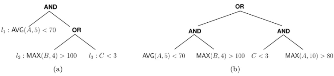
Figure 1: Two query tree examples: (a) aread-oncequery; (b) ashared query.
1
Introduction
There has been a recent explosion in the use of personal mobile devices for “mobile sensing” ap-plications. For instance, smartphones are equipped with increasingly sophisticated sensors (e.g., GPS, accelerometer, gyroscope, microphone) that enable near real-time sensing of an individual’s activity or environmental context. A smartphone can then perform embedded query processing on the sensor data streams, e.g., for social networking [5], remote health monitoring [6]. The continuous processing of streams, even when data rates are moderate (such as for GPS or ac-celerometer data), can cause commercial smartphone batteries to be depleted in a few hours [1]. It is thus crucial to reduce the amount of sensor data acquired for query processing, so as to reduce energy consumption and lengthen battery life.
In this work we study the problem of minimizing the expected sensor data acquisition cost (e.g., number of bytes, energy consumption due to byte transfers) when evaluating a query ex-pressed as a tree of arbitrarily composed conjunctive and disjunctive boolean operators applied to booleanpredicates. Each predicate is computed over data items from a particular data stream generated periodically by a sensor, and as a certain probability of evaluating to true. The eval-uation of the query stops as soon as a truth value has been determined, possiblyshortcircuiting part of the query tree. A “push” model by which sensors continuously transmit data to the device maximizes the amount of acquired data and is thus not practical. Instead, a “pull” model has been proposed [4], by which the query engine running on the device carefully chooses theorder and the numbers of data items to request from each individual sensor. This choice is based on a-priori knowledge of operator costs and probabilities, which can be inferred based on historical traces obtained for previous query executions. In practice, such intelligent processing is possible thanks to the programming and data filtering capabilities that are emerging on many wear-able sensor platforms (e.g., the SHIMMER platform [7]) so that data storage and transmission algorithms can be programmed “over the air.”
Two example query trees are shown in Figure 1, assuming streams namedA,B, andC, which are assumed to produce integer data items. Each leaf corresponds to a boolean predicate. A predicate may involve no operator, e.g., “C <3” is true if the last item from streamCis strictly lower than 3, or based on an arbitrary operator (in this exampleMAXorAVG) which is applied to a time-window for a stream, e.g., “AVG(A,5)<70” is true if the average of the last 5 items fromA is strictly lower than 70).
The problem of computing the truth value of a boolean query tree while incurring the mini-mum cost is known as ProbabilisticAND-ORTree Resolution (PAOTR) and has been studied extensively in the literature. In particular, [3] provides both a survey of known theoretical re-sults and several new rere-sults, all assuming that each data stream occurs in at most one leaf of the query tree. This assumption is termedread-once therein. In this case, forAND-trees (i.e., single-level trees with anANDoperator at the root node) a simpleO(nlogn) greedy algorithm
produces an optimal leaf evaluation order (nis the number of leaves in the query tree) [8]. For
DNFtrees (i.e., collections of AND-trees whose roots are the children of a singleORnode), a
O(nlogn) depth-first traversal of the trees that reuses the algorithm in [8] to order leaves within eachANDproduces an optimal evaluation order [3]. For generalAND-OR-trees the complexity of the problem is open. The example query tree in Figure 1(a) is a read-once query since no stream occurs in two leaves.
By contrast, in this work we study the more general case, which we termshared, in which a stream can occur in multiple leaves. The example in Figure 1(b) corresponds to a shared case since streamA occurs in two leaves. The device that processes the query acquires data items from streams and holds each data item in memory until that data item is no longer relevant. A data item from a stream is no longer relevant when it is older than the maximum time-window used for that stream in the query. Each time a leaf of the query must be evaluated, one can then compute the number of data items that must be retrieved from the relevant stream given the time-windows of the operator applied to that stream and the data items from that stream that are already in the device’s memory. For example, considering the query in Figure 1(b), assume the predicate “AVG(A,5) <70” is evaluated first, thus pulling 5 items from stream A. If later the predicate “MAX(A,10)>80” needs to be evaluated then only 5 additional items must be pulled.
Thesharedscenario is important in practice, and has been introduced and investigated in [4]. In that work the authors do not give theoretical results, but instead develop heuristics to deter-mine an order of operator evaluation that hopefully leads to low data acquisition costs. To the best of our knowledge, the complexity of the PAOTR problem in thesharedcase has never been addressed in the literature, likely because re-using stream data across leaves dramatically com-plicates the problem. When picking a leaf evaluation order, interdependences between the leaves must be taken into account. And in fact, even when a leaf evaluation order is given, computing the expected query cost is intricate while this same computation is trivial in theread-once case. In this work we study the PAOTR problem in theshared case and make the following con-tributions:
• ForAND-trees we give an optimal algorithm (which is much more involved than the optimal algorithm in theread-once case);
• ForDNF trees we show that the problem is NP-complete; but we are able to prove that there exists an optimal leaf evaluation order that is depth-first;
• For DNF trees we develop heuristics that we evaluate in simulation and compare to the optimal solution (computed via an exhaustive search) and to the heuristic proposed in [4]. In Section 2 we discuss models, the problem statement, and related work. We studyAND -trees andDNFtrees in Section 3 and Section 4, respectively. Section 5 concludes the paper with a brief summary of our findings and perspectives on future work. Detailed proofs of some of our theoretical results are provided in appendices.
2
Problem Statement and Examples
To define our problem we reuse the formalism and terminology in [3]. A query is anAND-OR tree, i.e., a rooted tree whose non-leaf nodes are ANDor ORoperators, and whose leaf nodes are labeled with probabilistic boolean predicates. Each predicate is evaluated over data items generated by a datastream. The evaluation of each predicate has a knownsuccess probability(the probability that the predicate evaluates toTRUE) and acost. In practice, the success probability can be estimated based on historical traces obtained from previous query evaluations. As in [3], we assume independent predicates, meaning that two predicates at two leaf nodes in a query
are statistically independent. The cost is determined by the number of data items required to perform the evaluation and the evaluation cost per data item for the stream. For instance, the cost of a data item could correspond to the energy cost, in joules, of acquiring one data item based on the communication medium used for the stream and the data item size.
More formally, we consider a set ofsstreams, S ={S1, . . . , Ss}. Stream Sk has a cost per
data item of c(Sk). A query on these streams, T, is a rooted AND-OR tree with m leaves,
l1, . . . , lm. Leaf lj has success, resp. failure, probability pj, resp. qj = 1−pj, and requires
the last dj items from stream S(j) ∈ S. The objective is to compute the truth value of the
root of the query tree by evaluating the leaves of the tree. Because each non-leaf node in a query tree is either an OR or an AND operator, it may not be necessary to evaluate all the leaves due toshortcircuiting. In other words, as soon as any child node of anOR, resp. AND, operator evaluates toTRUE, resp. FALSE, the truth value of the operator is known and can be propagated toward the root. For a given query, we define a schedule as an evaluation order of the leaves of the query tree, represented as a sorted sequence of the leaves.
We define thecostof a schedule as theexpected valueof the sum of the costs incurred for all leaves that are evaluated before the root’s truth value is determined. For instance, consider the query in Figure 1(a), in which leaves are labeledl1, l2, l3, and consider the schedulel2, l3, l1. The query processing begins with the acquisition of the data items necessary for evaluatingl2, which has cost 4·c(B). With probabilityp2,l2evaluates toTRUE, thus shortcircuiting the evaluation ofl3. Therefore, the expected evaluation cost of the ORoperator is: 4·c(B) +q2·c(C). If the
ORoperator evaluates toFALSE, which happens with probability q2q3, then the evaluation of
l1 is shortcircuited. Otherwise, l1 must be evaluated. The overall cost of the schedule is thus:
4·c(B) +q2·c(C) + (1−q2q3)·5·c(A). Recall that this query tree is for aread-once scenario.
The PAOTR problem consists in determing a schedule with minimum cost. The complexity of this problem is unknown in the read-once case for general AND-OR trees, while optimal polynomial-time algorithms are known forAND-trees [8] andDNF trees [3]. In this work, we focus on these two types of trees in theshared case, seeking to develop optimal algorithms or to show NP-completeness. We refer the reader to [3] for a detailed review of the PAOTR literature. To the best of our knowledge, the only work that has studied the shared case is [4], in which a heuristic is proposed for DNFtrees. We evaluate this heuristic in Section 4.4. In the next two sections we give examples of cost computations for an AND-tree and a DNF tree both in the shared case.
2.1
AND-tree example
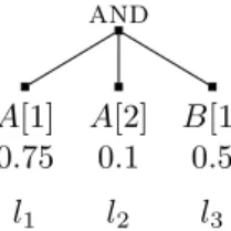
Consider the AND-tree query depicted in Figure 2 with three leaves labeled l1, l2, and l3, for
two streamsAandB. For each leaf (li), we indicate the stream (S(i)), the number of data items
needed from that stream to evaluate the leaf (di), and the success probability (pi). For instance,
leaf l2 requires d2 = 2 items from stream S(2) =A and evaluates to TRUE with probability
p2= 0.1. We assume that retrieving a data item from a stream has unitary cost, regardless of
and A[1] 0.75 l1 A[2] 0.1 l2 B[1] 0.5 l3
or
and1 and2 and3
A[1] l1 C[1] l3 D[1] l4 B[1] l2 C[1] l5 B[1] l6 D[1] l7
Figure 3: ExampleDNF tree.
the stream. There are 6 possible schedules for this tree, each schedule corresponding to one of the 3! orderings of the leaves. The optimal algorithm forread-once AND-trees sorts the leaves by non-decreasingdjc(S(j))/qj [8]. Because 1× c(A) q1 = 1 1−0.75 = 4, 2×c(A) q2 = 2 1−0.1 ≈2.22, and 1×c(B) q3 = 1
1−0.5 = 2, this algorithm schedules leaf l3 first. There are two possible schedules with l3 as the first leaf:
• l3, l1,l2 whose cost is: c(B) +p3×(c(A) +p1×c(A)) = 1 + 0.5×(1 + 0.75×1) = 1.875; and
• l3,l2,l1whose cost is: c(B) +p3×(2×c(A) +p2×0×c(A)) = 1 + 0.5×(2 + 0.1×0) = 2. However, another schedule,l1,l2,l3, has a lower cost: c(A) +p1×(c(A) +p2×c(B)) = 1 + 0.75×
(1 + 0.1×1) = 1.825. Therefore, the optimal algorithm for the PAOTR problem forread-once
AND-trees is no longer optimal in the shared case.
2.2
DNF tree example
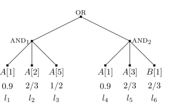
Figure 3 shows aDNFtree with threeANDnodes, for four streamsA,B,C, andD. Each leaf requires only one data item from a stream. Leaves are labeled l1 to l7, in the order in which they appear in a given schedule. This example is meant to illustrate the difficulty of the PAOTR problem in the case ofDNF trees in theshared scenario. In particular, computing the cost of a schedule is much more complicated than in theread-oncescenario due to inter-leaf dependencies. LetCj be the cost of evaluating leaflj, andC the overall cost of the schedule. We consider the
7 leaves one by one, in order:
Leafl1 –The first leaf is evaluated: C1=c(A).
Leaf l2 –This is the first leaf in itsAND, noANDhas been fully evaluated so far, and l2 is the first encountered leaf that requires streamB. Therefore, l2 is always evaluated, requiring a data item from streamB: C2=c(B).
Leafl3 –This is the second leaf from itsAND, noANDhas been fully evaluated so far, andl3
is the first encountered leaf that requires streamC. Therefore, a data item from C is acquired if and only ifl1 evaluates toTRUE: C3=p1c(C).
Leafl4 –This is the third leaf from its AND, noANDhas been fully evaluated so far, and l4
is the first encountered leaf that requires streamD. Therefore, one data item is acquired from
Dif and only if l1 andl3 both evaluate toTRUE: C4=p1p3c(D).
Leaf l5 – This is the second leaf from its AND, and AND1 has been fully evaluated so far.
However, one of the leaves of thatAND,l3, requires a data item that is also needed byl5, from
streamC. Ifl3 has been evaluated, then the evaluation cost ofl5is 0 because the necessary data
item fromC has already been acquired and is available “for free” when evaluatingl5. If l3 has not been evaluated (with probability 1−p1), it means thatAND1 has evaluated to FALSE.
streamC. We obtainC5= (1−p1)p2c(C).
Leaf l6 –Since l2 is always evaluated the data item from stream B required by l6 is always available for free: C6= 0.
Leafl7–This is the second leaf from itsAND, andAND1andAND2have been fully evaluated
so far. However, one of the leaves of AND1, l4, but none of those ofAND2, require the data
item that is needed by l7 from streamD. Therefore, l7 must be evaluated and its evaluation is not free if and only if l4 has not been evaluated, AND2 has evaluated toFALSE, and the
evaluation ofAND3went as far as l7. Therefore,C7= (1−p1p3)(1−p2p5)p6c(D).
Overall, we obtain the cost of the schedule:
T C = c(A) +c(B) + (p1+ (1−p1)p2)c(C)
+ (p1p3+ (1−p1p3)(1−p2p5)p6)c(D)
Given the complexity of the above cost computation, one might expect the PAOTR problem to be NP-complete in the shared case (recall that it is polynomial in the read-once case). We confirm this expectation in Section 4.
3
AND trees
In this section, we focus on AND-trees. We have seen in Section 2.1 that the simple greedy algorithm proposed in [8] in theread-oncecase is not optimal in thesharedcase. We propose an algorithm and we prove that it is optimal. This algorithm is still greedy but compares the ratios of cost to failure probability of all sequences of leaves that use the same stream, instead of only considering pair-wise leaf comparisons. We begin in Section 3.1 with a preliminary result on the optimal ordering of leaves that use the same stream.
3.1
Ordering same-stream leaves
In the example given in Section 2.1, we considered two schedules that begin with leaf l3. In the first schedule leaf l1 precedes l2, while the converse is true in the second schedule. Leaf
l1 requires one data item from stream A, while leaf l2 requires two data items from the same stream. Therefore the first schedule is always preferable to the second schedule: if we evaluate
l1beforel2and ifl1evaluates toFALSE, then there is no need to retrieve the second data item and the cost is lowered. A general result can be obtained:
Proposition 1. Consider an AND-tree and a leaf li that requires di data items from a stream S. In an optimal scheduleli is scheduled before any leaflj that requiresdj> di data items from
streamS.
Proof. See Appendix A for the proof.
3.2
Optimal schedule
Consider an AND-tree with m leaves, l1, . . . , lm, for s streams, S1, . . . , Ss. We define Lk =
{lj|S(lj) =Sk}, i.e., the set of leaves that require data items from streamSk. Algorithm 1 shows
a greedy algorithm (implemented recursively for clarity of presentation) that takes as input the
Lk sets, an initially empty scheduleξ, and an array of s integers,NItems, whose elements are
all initially set to zero. This array is used to keep track, for each stream, of how many data items from that stream have been retrieved in the schedule so far. Each call to the algorithm
appends to the schedule a sequence of leaves that require data items from the same stream, in increasing order of number of data items required. The algorithm stops when all leaves have been scheduled. The algorithm first loops through all the streams (thekloop). For each stream, the algorithm then loops over all the leaves that use that stream, taken in increasing order of the number of items required. For each such leaf the algorithm computes the ratio (variableRatio) of cost to probability of failure of the sequence of leaves up to that leaf. The leaf with minimum such ratio is selected (leaflj0 in the algorithm, which requiresdj0data items from streamS(lj0)). In the last loop of the algorithm, all unscheduled leaves that requiredj0 or fewer data items from streamS(lj0) are appended to the schedule in increasing order of the number of required data items.
Algorithm 1:GREEDY({L1, ...,Ls}, ξ, N Items)
if ∪s
i=1Li=∅then returnξ M inRatio←+∞
fork= 1 tosdoloop on streams
Cost←0
P roba←1
N um←N Items[k]
forlj inLk by increasingdj do
Cost←Cost+P roba×(dj−N um)×c(k)
P roba←P roba×pj
N um←dj
Ratio← Cost
(1−P roba)
if Ratio < M inRatiothen
M inRatio←Ratio j0←j forlj inLS(j0) by increasingdj do if dj≤dj0 then ξ.append(lj) LS(j0)← LS(j0)\ {lj} N Items[S(j0)]←dj0
returnGREEDY({L1, ...,Ls}, ξ, N Items)
Theorem 1. Algorithm 1 is optimal for the sharedPAOTR problem for AND-trees.
Proof. See Appendix B for the proof.
One may wonder how the optimal algorithm in the read-once case [8], which simply sorts the leaves by increasingdjc(S(j))/qj, fares in the shared case. In other terms, is Algorithm 1
really needed in practice? Figure 4 shows results for a set of randomly generated AND-trees. We define the sharing ratio, ρ, of a tree as the expected number of leaves that use the same stream, i.e., the total number of leaves divided by the number of streams. For a given number of leaves m= 2, . . . ,20 and a given sharing ratioρ = 1,5/4,4/3,3/2,2,3,4,5,10, we generate 1,000 random trees for a total of 157,000 random trees (note thatρ cannot be larger than the number of leaves). Leaf success probabilities, numbers of data items needed at each leaf, and per data item costs are sampled from uniform distributions over the intervals [0,1], [1,5], and [1,10], respectively. For each tree we compute the cost achieved by the algorithm in [8] and
40000
Cost
60
40
20
0
Shared instances sorted by increasing optimal cost
120000
80000
0
Algorithm in [9]
Optimal algorithm
Figure 4: Cost achieved by the algorithm in [8] and that achieved by the optimal algorithm, shown for each of the 157,000AND-tree instances sorted by increasing optimal cost.
that achieved by our optimal algorithm. Figure 4 plots these costs for all instances, sorted by increasing optimal cost. Due to this sorting, the large number of samples, and the limited resolution, the set of points for the optimal algorithm appears as a curve while the set of points for the algorithm in [8] appears as a cloud of points. The algorithm in [8] can lead to costs up to 1.86 times larger than the optimal. It leads to costs more than 10% larger for 19.54% of the instances, and more than 1% larger for 60.20% of the instances. The two algorithms lead to the same cost for 11.29% of the instances. We conclude that, in the shared case, Algorithm 1 provides substantial improvements over the optimal algorithm for theread-once case.
4
DNF Trees
In this section we considerDNFtrees. First, in Section 4.1 we provide a method for computing the expected cost of a given schedule for a DNF tree. In Section 4.2 we show that depth-first schedules are dominant, which means that there always exists a depth-depth-first schedule that is optimal. In Section 4.3, we then prove that the problem is NP-complete. This is in sharp contrast with the read-once case, in which a simple greedy algorithm is optimal [3]. In Section 4.4 we propose several heuristics to schedule aDNF tree and evaluate their performance on randomly generated problem instances.
4.1
Evaluation of a schedule
We have seen in Section 2.2 in an example that computing the cost of a schedule is non-trivial for DNF trees. In this section we formalize this computation. Consider a DNF tree with N ANDnodes, indexed i= 1, . . . , N. AND nodei hasmi leaves, denoted by li,j, j = 1, . . . , mi.
The probability of success of leafli,j is denoted bypi,j, and the stream that leafli,j requires is
denoted byS(i, j). We useLto denote the set of all the leaves. We consider a scheduleξ, which is an ordering of the leaves, and usels,t≺lu,v to indicate that leafls,t occurs before leaflu,vin ξ. We consider that the query is oversstreams,Sk,k= 1, . . . , s. The cost per data item ofSk
is denoted by c(Sk). We define the “t-th data item” of a stream as the data item produced t
time-steps ago, so that the first data item is the one produced most recently, the second is the one produced before the first, etc. In this manner, when we say that a leafli,j requiresdi,j data
items it means that it requires allt-th data items of the stream fort= 1,2, . . . , di,j.
Given the above, we define Lk,t as the set of the leaves that require the t-th data item
from streamSk, and that are the first of their respective AND nodes to require that data item.
Formally, we have: Lk,t= li,j∈ L S(i, j) =Sk, di,j≥t, and ∀r6=j, S(i, r)6=Sk ordi,r< t orli,j≺li,r
We also defineAi,j, the index set of allANDnodes that have been fully evaluated before a leaf li,j is evaluated, as:
Ai,j={k|mk =|{lk,r|lk,r≺li,j}|}.
If we useCi,j,tto denote the expected cost of retrieving thet-th data item of the relevant stream
when evaluating leafli,j, then the total costC of the scheduleξis:
C= N X i=1 mi X j=1 di,j X t=1 Ci,j,t.
The following proposition givesCi,j,t.
Proposition 2. Given a leafli,j that requires thet-th data item from stream Sk, if there exists rsuch that li,r ≺li,j andli,r∈ Lk,t, thenCi,j,t= 0. Otherwise:
Ci,j,t= Y lr,s∈Lk,t lr,s≺li,j 1− Y lr,u≺lr,s pr,u × Y a∈Ai,j 6∃r, la,r∈Lk,t 1− ma Y r=1 pa,r ! × Y li,u≺li,j pi,u ×c(S(i, j)).
4.2
Dominance of depth-first schedules
Theorem 2. Given a DNF tree, there exists an optimal schedule that is depth-first, i.e., that processes ANDnodes one by one.
Proof. Consider aDNFtreeT and a scheduleξ. Without loss of generality we assume that the AND nodes,A1, . . . , An, are numbered in the order of their completion. Thus, according toξ,A1
is the first AND node with all its leaves evaluated. We denote byM the number (possibly zero) of AND nodes thatξprocesses one by one and entirely at the start of its execution. Therefore, ifξ evaluates a leafli,j, withi6= 1, in them1 first steps, then M = 0. Finally, we assume that
the leaves of an AND node are numbered according to their evaluation order inξ.
We prove the theorem by contradiction. Let us assume that there does not exist a schedule that satisfies the desired property. Letξbe an optimal schedule that maximizesM. By definition ofM and by the hypothesis on the numbering of the AND nodes, scheduleξevaluates some leaves of the AND nodes AM+2, ...,An before it evaluates the last leaf ofAM+1. LetLdenote the set
of these leaves. We now define a new ξ0 which starts by executing at leastM + 1 AND nodes one by one:
• ξ0 starts by evaluating the first M AND nodes one by one, evaluating their leaves in the same order and at the same steps as inξ;
• ξ0 then evaluates all the leaves ofAM+1 in the same order as in ξ (but not at the same
steps);
• ξ0 then evaluates the leaves inL in the same order as inξ(but not at the same steps); • ξ0 finally evaluates the remaining leaves in the same order and at the same steps as inξ. The cost of a schedule is the sum, over all potentially acquired data items, of the cost of acquiring each data item times the probability of acquiring it. Letdbe a data item potentially needed by a leaf inT. We show that the probability of acquiringdis not greater withξ0 than withξ. We have three cases to consider.
Case 1)dis not needed by a leaf ofAM+1 and not needed by a leaf inL. Thend’s probability
to be acquired is the same withξandξ0.
Case 2)dis needed by at least one leaf ofAM+1. The only way in which a leaf that is evaluated
in ξ would not be evaluated inξ0 is if AM+1 evaluates toTRUE. By assumption, however, at
least one leaf ofAM+1 usesd. Therefore, for AM+1 to evaluate toTRUE,dmust be acquired.
Consequently, the probability thatdis acquired is the same withξand withξ0.
Case 3) dis needed by at least one leaf in L but not needed by any leaf of AM+1. ξ and ξ0
define the same ordering on the leaves inL. For each AND nodeAi, withM+ 2≤i≤N, there
is at most one leaf inAi∩ Lthat can be the leaf responsible for the acquisition ofdwithξ, and
it is the same leaf withξ0. LetF be the set of all these leaves. Then, withξ, the leaves inF are responsible for the acquisition ofdif and only if:
• A1, ...,AM all evaluate toFALSE;
• None of the evaluated leaves of A1, ...,AM needsd; and
• At least one of the leaves inF is evaluated.
Let us denote byP the probability that all the AND nodesA1, ...,AM evaluate toFALSEand
that none of the evaluated leaves of these AND nodes needs the data itemd. Let us denote by
D the probability thatdis acquired because of the evaluation of one of the leaves of the AND nodesA1, ...,AM. Finally, letRbe the probability that one of the leaves evaluated withξafter lM+1,mM+1 acquiresd, knowing that no leaves ofA1, ..., AM or in Lacquires it. Then, with ξ, the probabilitypthatdis acquired is:
p=D+P 1− Y li,j∈F 1− j−1 Y k=1 pi,k ! +R (1)
because leafli,j is evaluated with probabilityQ j−1
k=1pi,k, that is, if all the leaves from the same
AND node that are evaluated prior to it all evaluate toTRUE. The second term of Equation (1) is the probability that the leaves inF are responsible for acquiringd.
With scheduleξ0, the leaves ofF are responsible for the acquisition ofdif and only if: • The AND nodesA1, ...,AM, andAM+1 all evaluate toFALSE;
• None of the evaluated leaves of the AND nodesA1, ...,AM needd; and
• At least one of the leaves inF is evaluated. Thus, withξ0, the probabilityp0 that dis acquired is:
p0 = D + P 1− mM+1 Y k=1 pM+1,k ! × 1− Y li,j∈F 1− j−1 Y k=1 pi,k ! + R Comparing this equation with Equation 1, we see thatp0 is not greater thanp.
The probability that a data item is acquired withξ0is thus not greater than withξ. Therefore, in each of the three cases the cost ofξ0 is not greater than the cost ofξ, meaning thatξ0 is also an optimal schedule. Since ξ0 starts by executing at least M + 1 AND nodes one by one, we obtain a contradiction with the maximality assumption onM, which concludes the proof.
4.3
NP-completeness
In theread-oncecase, an optimal algorithm for DNF trees is built on top of the optimal algorithm forAND-trees [3]. The same approach cannot be used in theshared case, as seen in a simple counter-example (see Appendix D). And, in fact, in this section we show the NP-completeness of finding an optimal schedule to evaluate aDNFtree.
Definition 1 (DNF-Decision). Given a DNF tree and a cost bound K, is there a schedule whose expected cost does not exceedK?
Theorem 3. DNF-Decisionis NP-complete.
Proof. The NP-completeness is obtained via a non-trivial reduction from 2-PARTITION [2]. See the full proof in Appendix E.
4.4
Heuristics
Given the NP-completeness result in the previous section, we now propose several polynomial-time heuristics for computing a schedule. These heuristics fall into three categories, which we term leaf-ordered,AND-ordered, and stream-ordered.
Leaf-ordered heuristicssimply sort the leaves according to leaf costs (C), failure probabilities (q= 1−p), or the ratio of the two, which leads to three heuristics plus a baseline random one:
• Leaf-ordered, decreasingq(prioritizes leaves with high chances of shortcutting the evalua-tion of anANDnode);
• Leaf-ordered, increasingC (prioritizes leaves with low costs);
• Leaf-ordered, increasingC/q (prioritizes leaves with low costs and also with high chances of shortcutting the evaluation of anANDnode);
• Leaf-ordered, random (baseline).
The above first three heuristics have intuitive rationales. Other options are possible (e.g., sort leaves by decreasingC) but are easily shown to produce poor results in practice.
AND-ordered heuristics, unlike leaf-ordered heuristics, account for the structure of theDNF
optimal (Theorem 2). Furthermore, Algorithm 1 provides a way to compute an optimal schedule for the leaves within the same AND node. For this optimal schedule one can compute the (expected) cost and the probability of success of theANDnode using the method in Section 4.1 (this method actually applies to more general DNF trees). Therefore,AND-ordered heuristics simply order theANDnodes based on their computed costs (C), computed probability of success (p), or ratio of the two, and using Algorithm 1 for scheduling the leaves of each AND node, leading to three heuristics:
• AND-ordered, decreasing p (prioritizes AND’s with high chances of shortcircuiting the evaluation of theORnode);
• AND-ordered, increasingC (prioritizesAND’s with low costs);
• AND-ordered, increasingC/p(prioritizesAND’s with low costs and also with high chances of shortcircuiting the evaluation of theORnode);
There are two approaches to compute the cost of an ANDnode: (i) consider theANDnode in isolation assuming that theORnode has a singleANDnode child; or (ii) account for previously scheduledANDnodes whose evaluation has caused some data items to be acquired with some probabilities. We terms the first approach “static” and the second approach “dynamic,” giving us two versions of the last two heuristics above.
Stream-ordered heuristics proceed by ordering the streams from which data items are ac-quired, acquiring all items from a stream before proceeding to the next stream, until the truth value of the ORnode has been determined. This idea was proposed in [4], and to the best of our knowledge it is the only previously proposed heuristic for solving the PAOTR problem in the shared scenario for DNF trees. For each streamS the heuristic computes a metric, R(S), defined as follows:
R(S) =
P
i,j|S(i,j)=Sqi,jni,j
maxi,j|S(i,j)=Sdi,jc(S) ,
whereni,jis the number of leaf nodes whose evaluation would be shortcircuited if leafli,j was to
evaluate toFALSE. The numerator can thus be interpreted as the shortcutting power of stream
S. The denominator is the maximum data element acquisition cost over all the leaves that use stream S. The heuristic orders the streams by increasing R values. The rationale is that one should prioritize streams that can shortcut many leaf evaluations and that have low maximum data item acquisition costs. The heuristic as it is described in [4] acquires the maximum number of needed data items from each stream so as to compute truth values of all the leaves that require data items from that stream. In other words, the leaves that require data items from the same stream are scheduled in decreasing di,j order. However, Proposition 1 holds for DNF trees,
showing that it is always better to schedule these leaves in increasing di,j order. We use this
leaf order to implement this heuristic in this work. We have verified in our experiments that this version outperforms the version in [4] in the vast majority of the cases, with all remaining cases being ties.
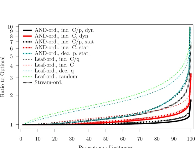
In total, we consider 4 leaf-ordered, 5 AND-ordered, and 1 stream-ordered heuristics. We first evaluate these heuristics on a set of “small” instances for which we can compute opti-mal schedules using an exponential-time algorithm that performs an exhaustive search. Such an algorithm is feasible because, due to Theorem 2, it only needs to search over all possi-ble depth-first schedules. Small instances are generated using the same method as that de-scribed in Section 3.2 for generating AND-tree instances. We generate DNF trees with N =
2, . . . ,9 ANDnodes and up to at most 20 leaves in total, generating 100 random instances for
each configuration, for a total of 21,600 instances (The source code is available at www.ens-lyon.fr/LIP/ROMA/Data/DataForRR-8373.tgz). For each instance we compute the ratio be-tween the cost achieved by each heuristic and the optimal cost. Figure 5 shows for each heuristic the ratio vs. the fraction of the instances for which the heuristic achieves a lower ratio. For
Ratio
to
Optimal
0
10
20
30
40
50
60
70
80
90
100
Percentage of instances
1
2
3
4
5
6
7
8
9
10
Stream-ord.
Leaf-ord., random
Leaf-ord., dec. q
Leaf-ord., inc. C
Leaf-ord., inc. C/q
AND-ord., dec. p, stat
AND-ord., inc. C, stat
AND-ord., inc. C/p, stat
AND-ord., inc. C, dyn
AND-ord., inc. C/p, dyn
Figure 5: Ratio to optimal vs. fraction of the instances for which a smaller ratio is achieved, computed over the 21,600 “small”DNFtree instances.
Ratio
to
AND-ord.,
inc.
C/p,
dyn
0
10
20
30
40
50
60
70
80
90
100
Percentage of instances
1
2
3
4
5
6
7
8
9
10
Stream-ord.
Leaf-ord., random
Leaf-ord., dec. q
Leaf-ord., inc. C
Leaf-ord., inc. C/q
AND-ord., dec. p, stat
AND-ord., inc. C, stat
AND-ord., inc. C/p, stat
AND-ord., inc. C, dyn
Figure 6: Ratio toAND-ordered increasingC/p dynamic vs. fraction of the instances for which a smaller ratio is achieved, computed over the 32,400 “large”DNFtree instances.
instance, a point at (80,2) means that the heuristic leads to schedules that are within a factor 2 of optimal for 80% of the instances, and more than a factor 2 away from optimal for 20% of the instances. The better the heuristic the closer its curve remains to the horizontal axis.
The trends in Figure 5 are clear. Overall the poorest results are achieved by the leaf-ordered heuristics, with the random such heuristic expectedly being the worst and the increasingC the best. The AND-ordered heuristics, save for the decreasing p version, lead to the best results overall. More precisely, the best results are achieved by sortingAND’s by increasingC/p, with sorting by increasingC leading to the second-best results. For the two AND-ordered heuristics that have both a static and a dynamic version, the dynamic version leads to marginally better results than the static version. Finally, the stream-ordered heuristic leads to poorer results than the best leaf-ordered heuristics, and thus significantly worse than the best AND-ordered heuristics.
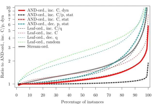
We also evaluate the heuristics on a set of “large” instances withN = 2, . . . ,10ANDnodes andm = 5,10,15,20 leaves perANDnode, with 100 random instances per configuration, for a total of 32,400 instances. For most of these instances we cannot tractably compute the optimal cost. Consequently, we compute ratios to the cost achieved by theAND-ordered by increasing
C/p dynamic heuristic, which leads to the best results for small instances. Results are shown in Figure 6. Essentially, all the observations made on the results for small instances still hold. We conclude that the best approach is to build a depth-first schedule, to sort theANDnodes by the ratio of their costs to probability of success, and to compute these costs dynamically, accounting for previously scheduledANDnodes.
5
Conclusion
Motivated by a query processing scenario for sensor data streams, we have studied a version of the Probabilistic And-Or Tree Resolution (PAOTR) problem [3] in which a data stream can be referenced by multiple leaves. We have given an optimal algorithm in the case of AND-trees and have shown NP-completeness in the case ofDNFtrees. ForDNFwe have shown that there is an optimal solution that corresponds to a depth-first traversal of the tree. This observation provides inspiration for a heuristic that largely outperforms the heuristic previously proposed in [4].
A possible future direction is to consider so-callednon-linear strategies [3]. Although in this work we have considered a schedule as a leaf ordering (called a linear strategy in [3]), a more general notion is that of a decision tree in which the next leaf to be evaluated is chosen based on the truth value of the previous evaluated leaf. A practical drawback of a non-linear strategies is that the size of the description is exponential in the number of tree leaves. In [3], it is shown that in theread-once case linear strategies are dominant for DNFtrees, meaning that there is always one optimal strategy that is linear. Via a simple counter example it can be shown that this is no longer true in theshared case (see Appendix F), thus motivating the investigation of non-linear strategies. Another possible future direction is to consider a less restricted version of the problem in which a single predicate at a leaf can access multiple streams rather than just a single one (e.g., “AV G(X <10)≥M IN(Y,20)”). There is no reason for real-world queries to be limited to a single stream per predicate. An interesting question is whether the PAOTR problem remains polynomial forAND-trees or whether it becomes NP-complete.
References
[1] S. Gaonkar, J. Li, R. Roy Choudhury, L. Cox, and A. Schmidt. Micro-Blog: Sharing and Querying Content through Mobile Phones and Social Participation. In Proc. of the ACM Intl. Conf. on Mobile Systems, Applications, and Services, 2008.
[2] M. R. Garey and D. S. Johnson. Computers and Intractability, a Guide to the Theory of NP-Completeness. W.H. Freeman and Company, 1979.
[3] Russell Greiner, Ryan Hayward, Magdalena Jankowska, and Michael Molloy. Finding Optimal Satisficing Strategies for And-Or Trees. Artificial Intelligence, 170(1):19–58, 2006.
[4] L. Lim, A. Misra, and T. Mo. Adaptive Data Acquisition Strategies for Energy-Efficient Smartphone-based Continuous Processing of Sensor Streams. Distributed Parallel Databases, 31(2):321–351, 2013.
[5] E. Miluzzo. Sensing Meets Mobile Social Networks: The Design, Implementation and Eval-uation of the CenceMe Application. InProc. of ACM Conf. on Embedded Networked Sensor Systems, 2008.
[6] I. Mohomed, A. Misra, M. Ebling, and W. Jerome. Context-Aware and Personalized Event Filtering for Low-Overhead Continuous Remote Health Monitoring. In Proc. of the IEEE Intl. Symp. on a World of Wireless Mobile and Multimedia Networks, 2008.
[7] The SHIMMER sensor platform. http://shimmer-research.com, 2013.
A
Proof of Proposition 1
Proof. We prove the proposition by contradiction. Consider anAND-tree and two leaves in the tree l1 and l2 that require data items from the same stream S such that d1 > d2. We terms these leaves “inverted” because the earlier one,l1, requires more data items than the later one,
l2. Assume that there is an optimal schedule ξin which l1 is scheduled before l2. Without loss of generality, we assume thatl1is the first leaf in the schedule that is part of an inverted pair of leaves (if not, consider the earliest such leaf). Evaluatingl2has always cost zero in this schedule because all data items required by l2 are also required byl1.
The sequence of leaves inξcan be written as: lb1, . . . , lbt, l1, lm1, . . . , lmu, l2, la1, . . . , lav. The costC ofξcan be written:
C=X+Pb·(d1−dLB)c(S) +Pb·p1·Y +Pb·p1· Pm·0 +Pb·p1· Pm·p2·Z where • Pb=Q t i=1pbi andPm= Qu i=1pmi;
• X is the expected cost of evaluating leaveslb1, . . . , lbt in that order;
• Y is the expected cost of evaluating leaves lm1, . . . , lmu in that order if leaves lb1, . . . , llt
andl1 all evaluate toTRUE;
• Z is the expected cost of evaluating leavesla1, . . . , lav in that order if leaveslb1, . . . , lbt,l1,
ll1, . . . , lmu, and l2 all evaluated toTRUE;
• dLB = maxi=1,...,t(dbi), or the number of elements of stream S that have been acquired
after evaluating leaveslb1, . . . , lbt.
Becausel1andl2 are the first two inverted leaves inξ,d1−dLB is non-negative (otherwise a leaf
amonglb1, . . . , lbt and leafl1would be inverted).
We now construct another schedule, ξ’, as lb1, . . . , lbt, l2, l1, lm1, . . . , lmu, la1, . . . , lav. The expected costC’ ofξ’ can then be written as:
C0=X+Pb·(d2−dLB)c(S) +Pb·p2(d1−d2)c(S) +Pb·p2·p1·Y +Pb·p2·p1· Pm·Z
Becausel1andl2 are the first two inverted leaves inξ,d2−dLB is non-negative (otherwise a leaf
amonglb1, . . . , lbt and leafl2 would be inverted). Computing the difference of the costs of both
schedules yields:
C − C0 =P
b(1−p2) ((d1−d2)c(S) +p1Y)
C − C0 is strictly positive because all costs are positives, all probabilities are between 0 and 1, and because d1> d2by assumption. This contradicts the optimality ofξ.
B
Proof of Theorem 1
Proof. We prove the theorem by contradiction. We assume that there exists an instance for which the schedule produced by Algorithm 1, ξgreedy, is not optimal. Among the optimal schedules,
let us pick a schedule,ξopt, which has the longest prefixPin common with scheduleξgreedy. We
consider the first decision (i.e., one recursive call to the algorithm) taken by Algorithm 1 that schedules a leaf that does not belong to P. Let k be the number of leaves scheduled by this decision, and let us denote themlσ(1), ..., lσ(k), scheduled in this order. Recall each call to the GREEDY algorithm schedules a sequence of leaves that all require data items from the same
stream. Furthermore, the scheduled sequence of leaves is a sub-sequence of the ordered sequence of all leaves that require data items from that stream, sorted by increasing number of data items required. Without loss of generality, we assume thatlσ(1), ...,lσ(k)all require items from stream
1. The first of these leaves may belong toP (as the last leaf occurrences inP). LetP0 be equal
toPminus the leaveslσ(1), ...,lσ(k). Then,ξgreedy can be written as:
ξgreedy=P0, lσ(1), ..., lσ(k),S. (2)
In turn,ξoptcan be writtenξopt=P0,Q,Rwherelσ(k)is the last leaf ofQ. In other words,Qcan
be written L1lσ(1)L2lσ(2)...Lklσ(k), where each sequence of leaves Li, 1≤i≤k, can be empty.
Note that, because of Theorem 1, and because the sequencelσ(1), ..., lσ(k) is a sub-sequence of
the the list of all leaves requiring data items from that stream sorted by increasing number of data items required, none of theLi sequences can contain a leaf requiring elements from stream
1. Therefore,
ξopt=P0,Q,RwhereQ=L1lσ(1)L2lσ(2)...Lklσ(k) (3)
Fromξgreedyandξopt, we build a new schedule,ξnew, defined as
ξnew=P0,NewOrder,RwhereNewOrder=lσ(1), ..., lσ(k), L1, ..., Lk (4)
P0,lσ(1), ...,lσ(k) is a prefix to bothξgreedy andξnew. This prefix is strictly larger thanP(since Pdoes not containlσ(k)). Therefore, if the cost of ξnew is not greater than that of ξopt, ξnew is
optimal and has a longer prefix in common withξgreedy than ξnew, which would contradict the
definition ofξopt. We obtain this contradiction by computing the cost ofξnew and showing that
it is no larger than that ofξopt.
Cost notations –To ease the writing of the proof we introduce several notations. If X is a
partial leaf schedule, P(X) denotes the probability that all leaves in Xevaluates toTRUE. In other words, P(X) = Qli∈Xpi. LetX and Y be two disjoint (partial) leaf schedules, i.e., they
do not have any leaf in common, such thatX is evaluated right before Y. Then Cost(Y | X)
denotes the cost of evaluatingY, assuming that all leaves in X have evaluated toTRUE. Of course,Cost(Y |X) takes into account all data items acquired during the successful evaluation
ofX. With these notations, we can now give the costs ofξnewandξopt based on their definitions
as sequences of partial leaf schedules in Equations (3) and (4): Cost(ξopt) =Cost(P0) +P(P0)Cost(Q|P0)
+P(P0)P(Q)Cost(R|P0,Q)
Cost(ξnew) =Cost(P0) +P(P0)Cost(NewOrder |P0)
+P(P0)P(NewOrder)Cost(R|P0,NewOrder)
BecauseQand NewOrder contain exactly the same leaves,P(Q) =P(NewOrder) and
Cost(R|P0,Q) =Cost(R|P0,NewOrder). Therefore,
Cost(ξopt)−Cost(ξnew) =P(P0) (Cost(Q|P0)−Cost(NewOrder |P0)) (5)
From what precedes, it now suffices to show that Cost(Q | P0)−Cost(NewOrder | P0) ≥0 to
prove the theorem.
Initial mathematical formulation –We use Proposition 1 to define notations that make it possible to obtain a simple expression for the quantity in Equation 5. Consider a streamS and two leaves li and lj that require, respectively, di and dj items from stream S, with di < dj.
Then, according to Proposition 1, li is always evaluated before lj in an optimal schedule. The GREEDY algorithm also schedules li before lj. If there does not exist any leaf lk requiring dk ∈[di;dj] elements from streams, then each time lj is evaluated, exactly dj −di items are
evaluated. In this case, we define ai as the number of data items that must be acquired when
evaluating leafli. Formally,
ai=di−max{dj |S(j) =S(i) anddj < di}
Remark: One should note that we can assume without loss of generality that theANDtree does not contain two leaves requiring the exact same number of items from the same stream. If such two leaves exist, then one replaces them by a single leaf with the same data item requirement and with a probability of success that is the product of the probability of success of the two original leaves. This is because once one of the two original leaves has been evaluated then the other one can be evaluated for free.
To ease the writing of the proof, we index the leaves in L1, ..., Lk according to the stream
from which they require data items, and introduce the following additional notations. LetNi be
the number of leaves inL1∪. . .∪Lk that require data items from streamiandli,j be thej-th
of these leaves. We then extend the notations defined in Section 2 as follows: the probability of success ofli,j is pi,j, li,j requires di,j elements from stream S(i, j), etc. µ(i,j) is the index of
the leaf sequenceLp to which leafli,j belongs: li,j ∈Lµ(i,j). Qi,j is the product of the success probabilities of the leaves that precedeli,jinLµ(i,j),Qmis the product of the success probabilities of all the leaves in Lm, andQm=Q
m
n=1Qn. Finally, we definePm =Q m
n=1pσ(n). With these
notations we can now write Cost(NewOrder |P0) as:
Cost(NewOrder |P0) = k X m=1 m−1 Y n=1 pσ(n) ! aσ(m) + s X i=2 Ni X j=1 k Y m=1 pσ(m) ! µ(i,j)−1 Y m=1 Qm Qi,jai,jc(S(i, j)) = k X m=1 Pm−1aσ(m)+ s X i=2 Ni X j=1
PkQµ(i,j)−1Qi,jai,jc(S(i, j)),
andCost(Q|P0) as:
Cost(Q|P0) = k X m=1 m−1 Y n=1 pσ(n) ! m Y n=1 Qn ! aσ(m) + s X i=2 Ni X j=1 µ(i,j)−1 Y m=1 pσ(m) µ(i,j)−1 Y m=1 Qm Qi,jai,jc(S(i, j)) = k X Pm−1Qmaσ(m)+ s X Ni X
Pµ(i,j)−1Qµ(i,j)−1Qi,jai,jc(S(i, j)).
Therefore:
Cost(Q|P0)−Cost(NewOrder |P0) = k X m=1 Pm−1Qmaσ(m) + s X i=2 Ni X j=1
Pµ(i,j)−1Qµ(i,j)−1Qi,jai,jc(S(i, j))
− k X m=1 Pm−1aσ(m)+ s X i=2 Ni X j=1
PkQµ(i,j)−1Qi,jai,jc(S(i, j)) = k X m=1 Pm−1(Qm−1)aσ(m) + s X i=2 Ni X j=1 Pµ(i,j)−1−Pk
Qµ(i,j)−1Qi,jai,jc(S(i, j)).
We introduce two additional notations:
α(i,j)=Qµ(i,j)−1 Pµ(i,j)−1−Pk Qi,j ,and A= Pk m=1Pm−1aσ(m) 1−Pk ,
so that we can finally write the expression for the difference of the two costs:
Cost(Q|P0)−Cost(NewOrder|P0) = k X m=1 Pm−1(Qm−1)aσ(m) ! + s X i=2 Ni X j=1 α(i,j)ai,jc(S(i, j)) . (6) Accounting for the algorithm’s scheduling decisions –The best decision for theGREEDY
algorithm was to evaluate at once the leaf sequence lσ(1), ..., lσ(k). Therefore, as far as the
algorithm is concerned, this was a better decision than evaluating any sequence of leaves from any other stream. More formally, for any streami, 2≤i≤s, and the set of the firstj leaves of that stream, 1≤j≤Ni, we have:
Pk m=1 Qm−1 n=1 pσ(n) aσ(m) 1−Qk m=1pσ(m) 1− j Y l=1 pi,l ! ≤ j X l=1 l−1 Y r=1 pi,r ! ai,lc(S(i, l)) ! .
These equations express the fact that these other sequence of leaves of aRatiovalue (see Algo-rithm 1) lower than that of the sequence scheduled by the algoAlgo-rithm, and can be rewritten as:
Ineq(i, j) : A 1− j Y l=1 pi,l ! ≤ j X l=1 l−1 Y r=1 pi,r ! ai,lc(S(i, l)) ! . (7)
Determining multiplying coefficients – To prove the theorem we combine the Inequali-ties (7) obtained for different values of i and j. The idea is to follow a variable elimination process. Ineq(i, Ni) is the only inequality in which ai,Ni appears. We multiplyIneq(i, Ni) by
Equation (6). Next, we multiplyIneq(i, Ni−1) by a valueλi,Ni−1 such that when adding the
resulting inequality to the one previously obtained, the coefficient ofai,Ni−1 is the same than in
Equation (6), and so on. This process can be done independently for the different streams as
Ineq(i, j) only contains terms relative to streami. We define theλi,j’s are defined as follows.
λi,j= α(i,Ni) QNi−1 l=1 pi,l ifj=Ni, α(i,j) Qj−1 l=1pi,l − α(i,j+1) Qj l=1pi,l otherwise.
We will later show that this choice of multipliers enable us to achieve our goal. However, as we want to use the λi,j’s as multiplying coefficients for inequalities, we must first show that they
are all non-negative. This is evident for theλi,Ni’s. Let us considerλi,j forj∈[1;Ni−1]:
λi,j = α(i,j) Qj−1 l=1pi,l − α(i,j+1) Qj l=1pi,l = 1 Qj−1 l=1pi,l µ(i,j)−1 Y m=1 Qm µ(i,j)−1 Y m=1 pσ(m) 1− k Y m=µ(i,j) pσ(m) Qi,j − 1 Qj l=1pi,l µ(i,j+1)−1 Y m=1 Qm µ(i,j+1)−1 Y m=1 pσ(m) 1− k Y m=µ(i,j+1) pσ(m) Qi,j+1 = 1 Qj−1 l=1pi,l µ(i,j)−1 Y m=1 Qmpσ(m) × 1− k Y m=µ(i,j) pσ(m) Qi,j− µ(i,j+1)−1 Y m=µ(i,j) Qmpσ(m) 1− k Y m=µ(i,j+1) pσ(m) Qi,j+1 pi,j
Let us first consider the case µ(i,j+1)=µ(i,j). Then the above equation can be rewritten:
λi,j = 1 Qj−1 l=1pi,l µ(i,j)−1 Y m=1 Qmpσ(m) 1− k Y m=µ(i,j) pσ(m) Qi,j− Qi,j+1 pi,j
By definition, Qi,j+1 is the product of the probabilities of success of all the leaves that are
evaluated before the leaf li,j+1 is evaluated. By definition of the numbering of the leaves, this
includes at least all the leaves that are evaluated before leafli,j is evaluated and leafli,j. As all
probabilities are less than or equal to 1, this implies that Qi,j+1 ≤Qi,jpi,j, and therefore that
λi,j≥0.
We now consider the other case: µ(i,j+1) > µ(i,j). Then, Qµ(i,j) is of the form Qi,jpi,jX whereX is the product of the probabilities of success of the leaves appearing inLµ(i,j) after the leaf li,j. Therefore, Qi,jpi,j ≥ Qµ(i,j). As for all i ∈ [1;s], 0 ≤pσ(i) ≤1,
Qk
m=µ(i,j+1)pσ(m) ≥ Qk
1−Qk
m=µ(i,j+1)pσ(m)≤1− Qk
m=µ(i,j)pσ(m),pσ(µ(i,j))(
Qµ(i,j+1)−1
m=µ(i,j)+1Qmpσ(m))Qi,j+1 ≤1 because it is a product of probabilities. Using these inequalities, we have:
1−Qk m=µ(i,j)pσ(m) Qi,j− Qµ(i,j+1)−1 m=µ(i,j) Qmpσ(m) 1− Qk m=µ(i,j+1)pσ(m) Q i,j+1 pi,j ≥ 1−Qk m=µ(i,j)pσ(m) Qi,j− Qµ(i,j+1)−1 m=µ(i,j) Qmpσ(m) 1− Qk m=µ(i,j)pσ(m) Q i,j+1 pi,j = 1−Qk m=µ(i,j)pσ(m) Qi,j− Qµ(i,j+1)−1 m=µ(i,j) Qmpσ(m) Q i,j+1 pi,j ≥ 1−Qk
m=µ(i,j)pσ(m) Qi,j−Qµ(i,j) pσ(µ(i,j))( Qµ(i,j+1)−1 m=µ(i,j)+1Qmpσ(m))Qi,j+1 1 pi,j ≥ 1−Qk
m=µ(i,j)pσ(m) Qi,j−Qµ(i,j)
1 pi,j
≥ 0
Therefore, all theλi,j’s are non-negative.
Combining the inequalities –For a given couple of values (i, j), with 2≤i≤sand 1≤j≤
Ni, letIneq(i, j) be Inequality (7) defined for (i, j). Because all theλi,j’s are non-negative, we
can form the inequality:
s X i=2 Ni X j=1 (λi,j×Ineq(i, j)) (8)
We now show that Inequality (8) leads to:
Cost(Q|P0)−Cost(NewOrder| P0)≥ k X m=1 Pm−1(Qm−1)aσ(m)+A s X i=2 Ni X j=1 α(i,j)(1−pi,j) (9)
To prove the Inequality (9), we consider the terms relative to streamiin Inequality (8):
Ni X j=1 (λi,j×Ineq(i, j)) ⇔ A Ni X j=1 λi,j 1− j Y l=1 pi,l ! ≤ Ni X j=1 λi,j j X l=1 l−1 Y r=1 pi,r ! ai,lc(S(i, l)) ! (10)
We start by considering the left-hand side of this inequality. Ni X j=1 λi,j 1− j Y l=1 pi,l ! = Ni−1 X j=1 λi,j 1− j Y l=1 pi,l ! +λi,Ni 1− Ni Y l=1 pi,l ! = Ni−1 X j=1 α(i,j) Qj−1 l=1 pi,l − α(i,j+1) Qj l=1pi,l ! 1− j Y l=1 pi,l ! + α(i,Ni) QNi−1 l=1 pi,l 1− Ni Y l=1 pi,l ! = Ni−1 X j=1 α(i,j) Qj−1 l=1 pi,l 1− j Y l=1 pi,l ! − Ni−1 X j=1 α(i,j+1) Qj l=1pi,l 1− j Y l=1 pi,l ! + α(i,Ni) QNi−1 l=1 pi,l 1− Ni Y l=1 pi,l ! = Ni−1 X j=1 α(i,j) Qj−1 l=1 pi,l 1− j Y l=1 pi,l ! − Ni X j=2 α(i,j) Qj−1 l=1pi,l 1− j−1 Y l=1 pi,l ! + α(i,Ni) QNi−1 l=1 pi,l 1− Ni Y l=1 pi,l ! = Ni X j=1 α(i,j) Qj−1 l=1pi,l 1− j Y l=1 pi,l ! − Ni X j=2 α(i,j) Qj−1 l=1pi,l 1− j−1 Y l=1 pi,l ! = α(i,1)(1−pi,1) + Ni X j=2 α(i,j) Qj−1 l=1pi,l 1− j Y l=1 pi,l ! − Ni X j=2 α(i,j) Qj−1 l=1pi,l 1− j−1 Y l=1 pi,l ! = α(i,1)(1−pi,1) + Ni X j=2 α(i,j) Qj−1 l=1pi,l j−1 Y l=1 pi,l− j Y l=1 pi,l ! = α(i,1)(1−pi,1) + Ni X j=2 α(i,j)(1−pi,j) = Ni X j=1 α(i,j)(1−pi,j) . Therefore, A Ni X j=1 λi,j 1− j Y l=1 pi,l ! =A Ni X j=1 α(i,j)(1−pi,j) . (11)
![Figure 4: Cost achieved by the algorithm in [8] and that achieved by the optimal algorithm, shown for each of the 157,000 AND-tree instances sorted by increasing optimal cost.](https://thumb-us.123doks.com/thumbv2/123dok_us/10223398.2926209/12.892.109.732.160.570/figure-achieved-algorithm-achieved-optimal-algorithm-instances-increasing.webp)