Advanced Column Generation Decompositions for Optimizing Provisioning Problems in Optical Networks

(1)

Advanced Column Generation Decompositions for

Optimizing Provisioning Problems in Optical Networks

Julian Enoch

A Thesis in

The Department of

Computer Science and Software Engineering

Presented in Partial Fulfillment of the Requirements for the Degree of

Master of Science (Computer Science) at Concordia University

Montréal, Québec, Canada

June 2018

c

(2)

C

ONCORDIA

U

NIVERSITY School of Graduate Studies

This is to certify that the thesis prepared

By: Julian Enoch

Entitled: Advanced Column Generation Decompositions for Optimizing Provi-sioning Problems in Optical Networks

and submitted in partial fulfillment of the requirements for the degree of

Master of Science (Computer Science)

complies with the regulations of this University and meets the accepted standards with respect to originality and quality.

Signed by the Final Examining Committee:

Chair Dr. Sudhir Mudur External Examiner Dr. Thomas G. Fevens Examiner Dr. Lata Narayanan Supervisor Dr. Brigitte Jaumard Administrative Supervisor Dr. Chadi Assi Approved by

Sudhir Mudur, Chair

Department of Computer Science and Software Engineering

2018

Amir Asif, Dean

(3)

Abstract

Advanced Column Generation Decompositions for Optimizing Provisioning Problems in Optical Networks

Julian Enoch

With the continued growth of Internet traffic, and the scarcity of the optical spectrum, there is a continuous need to optimize the usage of this resource. In the process of provisioning optical networks, telecommunication operators must deal with combinatorial optimization problems that are NP-complete. One of these problems is theRouting and Wavelength Allocation(RWA) which considers the fixed frequency grid, and theRouting and Spectrum Allocation(RSA) which is defined for the flexible frequency grid. While the flexible frequency grid paradigm attempted to improve the spectrum usage, the RSA problem has an additional spectrum dimension that makes it harder than the RWA problem.

In this thesis, in continuation of the previous studies, and using the advanced techniques of

Integer Linear Programing, we propose aColumn Generationalgorithm based on aLightpath de-composition which we implement for both the RWA and the RSA problems. This algorithm proved to be the most efficient so far producing optimal or near optimal solutions, and improving the com-putation times by two orders of magnitude on average. This algorithm is based on the approach of finding the right decomposition scheme as to be able to solve thePricing Problemin a polynomial time. This approach can be used in other optimization problems.

In addition, we consider the sameConfigurationdecomposition as the previous studies, and we propose an algorithm based onNested Column Generation. We implemented this algorithm for both the RSA and the RWA problems, which led to a considerable improvement on the previous algo-rithms that use the sameConfigurationdecomposition. ThisNested Column Generationapproach

(4)

Acknowledgments

I would like to acknowledge the people who:

- Strive to be better by hard work and self-disipline;

- Respect the right of other people to their integrity just as they claim the right to the same; - Work with responsibility, honesty and fairness toward their organization and collaborators.

(5)

List of Figures

Figure 2.1 Flow chart of the L_CG Algorithm for RWA. . . 12

Figure 2.2 Computation of the Initial Set of Columns . . . 15

Figure 2.3 Characteristics of the Selected Lightpaths . . . 18

Figure 3.1 Flow chart of the L_CG for RSA . . . 25

Figure 3.2 Spain network topology . . . 26

Figure 4.1 RWA wavelengthConfiguration. . . 30

Figure 4.2 Nested Column Generation Flow for RWA . . . 34

Figure 5.1 Configurationillustration . . . 41

Figure 5.2 Nested Column Generation Flow for RSA . . . 43

Figure A.1 A binomial tree of order n = 3 for a node pair with 3 atomic requests . . . . 54

Figure D.1 NSF network topology . . . 60

Figure D.2 USA network topology . . . 61

Figure D.3 NSF network topology . . . 61

Figure D.4 NTT network topology . . . 62

Figure D.5 ATT network topology . . . 62

(9)

List of Tables

Table 2.1 Characteristics of the Datasets . . . 16

Table 2.2 Computational comparisons . . . 17

Table 3.1 Comparative Model/Algorithm Performance . . . 27

Table 3.2 Numerical results for new datasets . . . 28

Table 4.1 W_NCG Algorithm Results and Comparison . . . 38

Table 5.1 ICTON dataset - Solution and Comparison . . . 47

Table 5.2 INOC dataset - Algorithm Results and Performance. . . 49

(10)

Chapter 1

Introduction

1.1 Motivation

According to the latest report ofCisco[2017], the annual global IP traffic in 2016 was 1.2 Zetta-Byte, and is expected to increase threefold by 2021. This growth is driven in a large proportion by the IP video traffic which would account for 82% of all IP traffic by then. In particular, applications such as Live Internet video, Virtual Reality, Internet gaming will contribute for the largest growth portion. This continuous growth in the demand translates into a continuous need to enhance the design and the engineering of the networking infrastructure and technologies.

The core networks of Internet (called also long-haul networks) are based on optical technology and their links are made of optical fibers. These long-haul networks cover in general entire conti-nents and their links span hundreds if not thousands of kilometers. As a way to increase the capacity, these networks implement Wavelength Division Multiplexing (WDM), where the idea is to trans-mit data simultaneously at multiple carrier wavelengths (or, equivalently, frequencies) over a fiber. Traditionally, the multiplexing was done according to a Coarse WDM frequency grid (called fixed grid) where the carrier wavelength granularity is 50 GHz. As of 2012, the International Telecom-munication Union issued a new recommendation that defines a flexible Dense WDM frequency grid (flexible grid for short) with a finer frequency granularity of 12.5 GHz called a frequency slot [IUT, 2012]. This evolution has allowed the emergence of Elastic Optical Networks.

(11)

The main phase in the process of designing an optical network is concerned with traffic provi-sioning. In all instances, traffic provisioning consists of assigning a routing path, and allocating a frequency range to each traffic demand. In the case of fixed grid, the frequency range corresponds to a wavelength. In this case, the provisioning problem is called theRouting and Wavelength Al-location problem. In the case of flexible grid, the frequency range corresponds to a number of contiguous frequency slots. In this case, the provisioning problem is called theRouting and Spec-trum Allocationproblem.

1.2 Objectives and contributions

Although the flexible grid was introduced to allow a more economic use of the optical resources, the fixed grid remains in use in a lot of optical networks for many reasons such as the low cost of the optical devices and the simplicity of the engineering algorithms. Hence, this thesis discusses both RWA and RSA problems.

Among the existing algorithms for these problems, heuristics are in general fast but they do not provide any guarantee on the quality of the solutions. On the other hand, exact algorithms do not scale well, and are usually used on small network instances.

Our objective is to propose exact algorithms with better scalability than the existing ones, as to allow the resolution of real-life network instances. In doing so, we use a large scale optimization technique calledColumn Generation. While using RWA and RSA as study cases, we explore the possibility to maximize the potential ofColumn Generationby finding the ideal decomposition of these problems. In doing so, we designed two algorithms:

(1) The first algorithm employs aLightpathdecomposition combined with aColumn Generation

scheme

(2) The second algorithm employs aConfigurationdecomposition combined with aNested Col-umn Generationscheme

(12)

• L_CG refers to aColumn Generationalgorithm using aLightpathdecomposition introduced in this thesis for both RWA and RSA;

• C_NCG refers to aNested Column Generationalgorithm using aConfiguration decomposi-tion introduced in this thesis for RSA;

• W_NCG refers to aNested Column Generationalgorithm using aConfiguration decomposi-tion introduced in this thesis for RWA;

• C_CG refers to aColumn Generationalgorithm using aConfigurationdecomposition intro-duced byJaumard and Daryalal[2016] for RSA;

• W_CG refers to aColumn Generationalgorithm using a wavelength Configuration decom-position introduced byJaumard and Daryalal[2017] for RWA;

All the implementations were coded in Java and the Branch-and-Bound part was done using CPLEX. Shortest path calculation was done with an open-source Java library JGraphT implementing Dijkstra’s algorithm. The results were produced on a 3.6-4.0 GHz 4-core machine with 32 GB of memory.

We were able to publish part of our work, and we are in the process of publishing the remaining part. Therefore in Chapter2, we present the paper [Enoch and Jaumard,2018a] which uses a Light-pathdecomposition to solve the RWA problem. Chapter3presents the paper [Enoch and Jaumard, 2018b] which uses a similar decomposition applied to the RSA problem. Chapter4introduces the more advancedNested Column Generationapproach applied to the RWA problem. Chapter5shows the results obtained when applyingNested Column Generationto the RSA problem.

Next, we factored out the literature review of the two optimization problems discussed in this thesis.

(13)

1.3 Literature Review

1.3.1 Routing and Wavelength Assignment

While we are interested in the so-called max RWA problem in this study, many studies consider the min RWA. In the max RWA problem, the objective is to maximize the number of granted re-quests, i.e., it corresponds to a provisioning problem. On the other hand, in the min RWA problem, the objective is to minimize the number of required wavelengths in order to grant all the requests, hence it corresponds to a dimensioning problem.

The max RWA problem has been extensively studied in various flavours. In order to set the stage for the present work, we provide the key references on the past works that have studied the RWA problem with the objective to maximize the GoS, using Integer Linear Programming, in an attempt to solve it exactly, or nearly exactly with an estimate of the accuracy. We also provide few references related to the min RWA as it is a very similar problem.

The first class of studies used link based models. Such models are considered to be compact for they have a polynomial number of variables and constraints. Yet, none of them is scalable for large network instances.Jaumard et al.[2007] provide an extensive review of the different proposed link models.

The second class of studies considered path based models, see, e.g., [Saad and Luo, 2002]. Therein, the authors used a Lagrangian decomposition to show that the LP relaxation can be solved in polynomial time, but the ILP itself was solved using a pre-computed subset of paths, which makes the model, and therefore the algorithm non-exact. Other path formulations were explored in the context of the min RWA problem, see, e.g., [Christodoulopoulos et al.,2010;Liu and Rouskas, 2012].

The need for scalable and exact ILP models triggered the introduction of advanced models that can make use of decomposition techniques. While providing a review of the existing CG algorithms, Jaumard et al.[2009] hinted to an exact column generation (CG) model and CG-ILP algorithm with a polynomial-time pricing problem (i.e., generator of lightpaths). However, the authors refrained from pursuing this direction, arguing that it suffers from a wavelength symmetry issue and an optimal LP relaxation that is not better than the one of the link formulations. Indeed,

(14)

an integer linear program (ILP) is symmetric if its variables can be permuted without changing the structure of the problem. Symmetry is usually viewed as the prelude of great difficulties for solving exactly an ILP with traditional branch-and-bound, branch-and-cut or branch-and-price algorithms [Margot,2010]. Still, we decided to revisit the lightpath decomposition model following its good performances for the RSA problem [Enoch and Jaumard,2018b].

In the prospect of improving the characteristics of the path model, many studies considered new ILP formulations with coarse variables, where each variable is associated with wavelength Con-figuration, i.e., a set of lightpaths all routed with the same wavelength. This led to the so-called Independent Set (IS) (also called Independent RoutingConfigurationdecomposition (IRC)) mod-els, using an underlying graph in which each node is associated with a path, and two nodes are connected if their associated paths share a link. Finding a wavelengthConfigurationis equivalent to identifying an independent set (also called stable set). Ramaswami and Sivarajan[1995] intro-duced a firstIndependent Set(IS) model and solved its linear relaxation to obtain an upper bound while explicitly enumerating the exponential number of variables. Lee et al.[2000] introduced a slightly more compact model thanRamaswami and Sivarajan[1995], resulting in the so-called In-dependent RoutingConfiguration decomposition model and solved it using a column generation algorithm where the pricing problem is written as a weighted independent set problem, with an ex-ponential number of variables. Two years later,Lee et al.[2002] proposed to solve the same pricing problem using an embedded branch-and-price technique, which is quite computationally expensive. Jaumard et al.[2009] then proposed to model the pricing problem as a multi-flow problem using a link formulation, thus overcoming the issue of the exponential number of variables in the pricing problem. More recently, Jaumard and Daryalal[2017] improved the scalability ofJaumard et al. [2009] combining the link formulation of the pricing problem with a path one in order to speed up the generation of wavelength Configurations. The resulting algorithm is able to solve efficiently data instances with up to 90 nodes (ATT network) and up to 150 wavelengths (USA, Germany and NTT networks).

While it was proved byJaumard et al.[2009] that a wavelength decomposition ILP model could theoretically provide a better LP relaxation bound than the lightpath decomposition, it is usually not the case on classical data instances. Therefore, while providing a better LP bound in general,

(15)

additional complexity is put on the pricing problems, and impact the computational times as will be seen in Section2.4. In the current work, we revisit the lightpath decomposition, and compare its performances on the same instances as [Jaumard and Daryalal,2017]. We show that despite its wavelength symmetry, we are able to produce significantly better results than the latest Maximum Independent RoutingConfigurationdecomposition proposed model and algorithm ofJaumard and Daryalal[2017] both in terms of solution quality and algorithm efficiency.

1.3.2 Routing and Spectrum Assignment

Various mathematical models have already been proposed for solving the RSA problem, includ-ing several column generation models, however with different decomposition schemes, and different solution processes. All classical Integer Linear Programming (ILP) models are not scalable and can only solve very small data instances.

We now review the column generation models. Ruiz et al. [2013b] proposed a first column generation model, with the minimization of the number of denied demands and the amount of unserved bit-rate. They are able to solve data instances with up to 96 slots, and an overall demand distributed over a set of 180 node pairs in the Spain network (21 nodes). Klinkowski et al.[2014] improved the formulation ofRuiz et al.[2013b] with the use of valid inequalities (cuts), but did not go significantly farther than in [Ruiz et al.,2013b].Klinkowski and Walkowiak[2015] reformulated the RSA problem as a mixed-integer program and solved it using a branch-and-price algorithm. In order to enhance the performance of their algorithm, a simulated annealing-based heuristic was added. In a recent attempt to exactly solve large-size instances of RSA problem,Klinkowski et al. [2016] proposed a branch-and-price algorithm. However, the resulting algorithm is not an exact algorithm and the LP (Linear Programming) value is not a valid bound to assess the quality of the ILP solutions, as the authors use pre-computed lightpaths, and consequently did not consider, explicitly or implicitly, all possible lightpaths.

In this study, we propose an ε-optimal solution scheme, i.e., an algorithm that outputs an ε -solution. The addition of a branch-and-price algorithm would make it possible to reach an optimal solution.

(16)

Chapter 2

Enhanced RWA Exact Solution with a

New Lightpath Decomposition

Algorithm

Enoch and Jaumard[2018a]. Enhanced RWA exact solution with a new lightpath decomposition algorithm. In IEEE International Conference on Computing, Networking and Communications -ICNC.

2.1 Introduction

The Routing and Wavelength Assignment (RWA) problem is concerned with the provisioning of fixed-grid Wavelength Division Multiplexing (WDM) optical networks.

Despite the recent introduction of the flexible WDM grid, the RWA problem is still of great in-terest for many reasons [Saleh and Simmons,2011,2012;Simmons,2017;Muciaccia and Passaro, 2017]. While flexible grids are widely investigated and moved forward, they add significant network management cost and complexity, e.g., the requirement of many bandwidth-variable transponders together with the need to track how the spectrum is sliced up on each fiber [Simmons, 2017]. In addition, the advantage of the flexible grid over the fixed grid is very much dependent on the gran-ularity of the demands in terms of bandwidth: while it may offer up to a 1.5 effective capacity

(17)

multiplier for heavy granularities (400 Gbs and higher) [Simmons,2017], it offers no significant advantages for low granularities in view of its additional network costs and complexities.

We revisit the static RWA problem that consists of provisioning a set of demands over a set of lightpaths subject to the wavelength continuity constraint (i.e., an all-optical wavelength chan-nel between two nodes, which may span more than one fiber link). We consider the objective of maximizing the Grade-of-Service (GoS), which is suitable for the provisioning phase of network management, as opposed to the objective of minimizing the number of required wavelengths, which is involved in the dimensioning phase. These two objectives lead to the so-called max-RWA and min-RWA problems, respectively.

Under these assumptions, given a WDM network and a traffic demand matrix, the RWA problem consists of assigning a routing path and one wavelength to each unit of traffic connection as to maximize the number of granted connections, while avoiding any wavelength clash on a link and a wavelength simultaneously. This problem has been extensively studied since its inception [Zang et al.,2000;Jaumard et al.,2007], yet, with the unrelentingly growing traffic demand on Internet, there is a need to further improve the solution of large and practical network instances.

Among the previous studies of the RWA problem, the heuristics are of practical use for their scalability, but they do not provide any information on the quality of their solution, see, e.g., [ Jau-mard et al.,2006;Noronha and Ribeiro,2006;Duhamel et al.,2016]. On the other hand, algorithms for solving exact models, using ILP (Integer Linear Programming) solvers, produce in general near optimal solutions, with an estimate of the accuracy of the solution. In this work, we propose an exact lighpath decomposition model and anε-optimal algorithm. We aim to improve upon the quality and the efficiency of the previous existing studies. In doing so, the proposed lightpath decomposition model will be solved using column generation (CG) techniques with a polynomial-time lightpath generator. This contrasts with previously proposed decomposition schemes, e.g., with wavelength

Configurations[Jaumard and Daryalal,2017], in which symmetry was eliminated at the expense of a non-polynomial algorithm for generating wavelengthConfigurations.

The paper is organized as follows. We define the notations and state the lightpath decomposition ILP model in Section2.2. Next, in Section2.3, we describe precisely the L_CG algorithm to solve it efficiently. Performances of the L_CG algorithm is extensively evaluated in Section2.4, and

(18)

shown to be significantly faster than the best currently available RWA algorithms. Conclusions are drawn in the last section.

2.2 L_CG: Lightpath Decomposition Model

We assume a transparent All-Optical Network (AON), and we consider the general case of asymmetrical traffic.

We propose a lightpath-based model similar to the one introduced in [Lee et al.,2002]. It differs from the path formulation studies, e.g., [Jaumard et al.,2009;Liu and Rouskas,2012], in that the variables are indexed by both a path and a wavelength.

Consider a WDM optical network represented by a directed graphG= (V, L)whereV repre-sents the nodes of the network, andLis the set of links representing the directional optical fibers. The optical spectrum is divided into a set of wavelengths with equal capacity, denoted byΛ. The traffic can be viewed as a|V| × |V|matrix where each elementDsdrepresents the number of

wave-length units from a source nodevsto a destination nodevd. LetSDbe the set of node-pairs with

traffic.

For a given node-pair(vs, vd) ∈ SD, we define aLightpathπ as the routing path of a traffic

connection fromvs to vdon a given wavelength λ ∈ Λ. LetΠ be the set of all lightpaths π for

all pairs inSD. The decision variablexπ determines whether lightpathπ is retained in the optimal

solution. We define the following parameters:

- asd_π : indicates if lightpathπserves a unit connection(vs, vd)∈ SD.

- bλ_π`: indicates if lightpath π is routed on wavelength λ ∈ Λ and a path that contains link `∈L.

The ILP model reads as follows:

z = max X

π∈Π

(19)

subject to: X π∈Π asd_π xπ ≤Dsd (vs, vd)∈ SD (2.2) X π∈Π bλ_π`xπ ≤1 `∈L, λ∈Λ (2.3) xπ ∈ {0,1} π ∈Π. (2.4)

Constraints (2.2) ensure that the number of connections from a source to a destination does not exceed the actual demand. Constraints (2.3) mean that each wavelength on each link is used by at most one connection.

Note that the above model remains valid even in a network with multi-fiber links. It suffices to build a graph, which is a multi-graph, where each link is associated with one fiber link.

2.3 Solution Design

After reviewing very briefly the characteristics of a column generation algorithm, we describe in detail the L_CG algorithm we used for solving the lightpath decomposition model that was proposed in the previous section.

2.3.1 Column Generation Framework

Given the exponential number of columns - lightpaths - in the proposed model, we resort to the Column Generation method [Gilmore and Gomory, 1961] to solve its linear relaxation, and then derive an integer solution. This technique consists of decomposing the original problem into a Restricted Master Problem - RMP - (i.e., model (2.1) - (2.4) with a very restricted number of variables) and one or several pricing problems - PPs. In the particular case of model (2.1) - (2.4), we will show in the next section that the pricing problem can be decomposed into |V|2 _{× |}_Λ_| independent smaller pricing problems, each denoted by PPsd,λ. The RMP and the PP(s) are solved

alternately. Solving the RMP consists in selecting the best lightpaths, while solving the PPs allows the generation of improving potential lightpaths, i.e., lightpaths such that, if added to the current

(20)

RMP, improve the optimal value of its linear relaxation. The process continues until the optimality condition is satisfied, that is, all the so-called reduced costs that define the objective function of the pricing problems are negative, see [Chvatal,1983] if not familiar with linear programming concepts. Once the optimal solution of the linear relaxation has been reached, we derive an integer solu-tion by solving exactly the last RMP with integrality requirements. This leads to an integer solusolu-tion, denoted byz˜ILP. This last value is not necessarily the optimal value, but we can easily compute its

accuracyε. As we will see with the numerical results in Section2.4, the accuracy gap is small, so we decided not to resort to a solution scheme, such as, e.g., a branch-and-price algorithm [Barnhart et al., 1998], in order to compute an integer optimal solution. Indeed, while a branch-and-price algorithm would allow to compute an optimal integer solution, it would require much more com-putational resources, which is not justified in view of the very good accuracy of the solutions in practice (see Section2.4).

The accuracy (ε) of the integer solution, derived by solving exactly the ILP model associated with the last RMP, is defined as follows:

ε= z ? LP−z˜ILP ˜ zILP , (2.5) wherez?

LPandz˜ILPdenote the optimal LP value and the optimal ILP value of the last RMP,

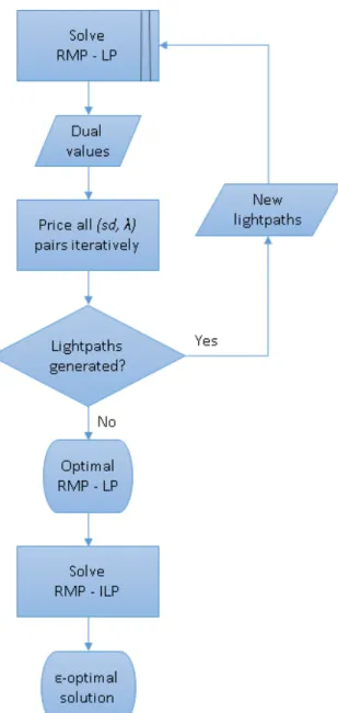
respec-tively. The solution process is illustrated in the flowchart of Figure2.1.

Before any LP re-optimization, we solve the whole series of pricing problems, where each pricing problem PPsd,λis associated with one node pair and one wavelength.

After each re-optimization of the RMP, we eliminate the variables that are not in the basis, as described in [Chvatal,1983]. While we may need to regenerate some of the eliminated columns (but they are not expensive to generate), it helps to maintain a reasonable number of variables, indeed equal to the number of constraints. Moreover, before deriving an ILP solution, i.e., solving exactly the last RMP subject to integer requirements, we remove all variables which are equal to zero, i.e., not contributing to the value ofz?

(21)

(22)

2.3.2 Decomposition of the Pricing Problem

We, next, show that the column generation decomposition involves a set of independent elemen-tary pricing problems, denoted by PPsd,λ, one for each node pair and wavelength.

Letµsd ≥ 0 andµλ_` ≥ 0be the values of the dual variables associated with constraints (2.2)

and (2.3), respectively. For a given vertexv∈V, we denote byω−(v)(respectivelyω+(v)) the set of ingoing (respectively outgoing) links. The objective of the pricing problem PP is defined by the reduced value [Chvatal,1983] and can be written as follows.

[PP] max 1− X (vs,vd)∈SD µsdasdπ − X `∈L X λ∈Λ µλ_` bλ_π`. (2.6) subject to: X (vs,vd)∈SD asd_π = 1 (2.7) X `∈ω−₍_v s) bλ_π` = X `∈ω+₍_v d) bλ_π` =asd_π λ∈Λ,(vs, vd)∈SD (2.8) X `∈ω−₍_v₎ bλ_π`= X `∈ω+₍_v₎ bλ_π` λ∈Λ,(vs, vd)∈SD, v ∈V \ {vs, vd} (2.9) asd_π ∈ {0,1} (vs, vd)∈SD (2.10) bλ_π`∈ {0,1} λ∈Λ, `∈L. (2.11)

The set of constraints corresponds to flow constraints in order to determine a path for each (vs, vd)and eachλ.

The objective of the Pricing Problem is to find a lightpath that optimizes the reduced value. Instead of generating only one optimal lightpath, we will compute all feasible lightpaths for which the reduced value is positive, in a multi-column generation scheme.

Given the wavelength continuity constraint, i.e., each lightpath must be routed on only one wavelength, it is possible to fix the wavelength and solve multiple smallerPricing Problems, one for each wavelength, sequentially.

(23)

Pricing Problemfurther into sequential smaller problems, by fixing the node-pair at each iteration (i.e., by settingasd_π to 1 for the current node-pair and to 0 for all the others).

Thus, rather than solving the pricing problem as a whole using an ILP solver, it is of interest to decompose it into|SD| × |Λ|independent smaller pricing problems PPsd,λ, whose reduced value is

defined as follows:

[PPsd,λ] max 1−µsd−

X

`∈L

µλ_` bλ_π`. (2.12)

For a given(vs, vd), the first terms of the reduced value, i.e.,1−µsd is a constant. Hence, the

maximization of the reduced value is equivalent to:

[PPsd,λ] min

X

`∈L

µλ_` bλ_π`. (2.13)

Taking into account that the set of constraints amounts to a set of flow constraints for a given node pair and wavelength, each pricing problem PPsd,λis equivalent to a shortest-path problem with

non-negative weightsµλ_`, for`∈L.

As a result of this decomposition, we are able to solve the pricing problem using |SD| × |Λ|

times a polynomial-time graph algorithm (e.g., Dijkstra [Ahuja et al.,1993]), instead of an ILP. As we will see in Section2.4, this approach yields substantial increase of efficiency.

2.3.3 Initial Set of Columns

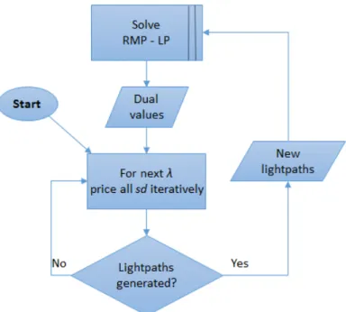
We propose a symmetry breaking initialization, solving in sequence the various pricing prob-lems and re-optimizing the RMP more often than in the steady state, as described in the flowchart of Figure2.2.

Initially, the first RMP is empty and all its dual values are null. This implies that, for each unit connection(vs, vd), the first series of pricing problems will compute a shortest path in terms of the

number of hops only. In order to avoid getting the same lightpaths for a given node pair, for all the wavelengths, we need to be cautious and therefore re-optimize the RMP more often.

Indeed, in the beginning of the column generation process, we solve all the elementary pricing problems PPsd,λfor a givenλ. After eachλround, we re-optimize the current RMP, which produces

(24)

Figure 2.2: Computation of the Initial Set of Columns

new dual values. Those are then used in the elementary pricing problems for the next wavelength, see Figure2.2) for the details.

The combination of (i) the generation of an initial set of columns,(ii)the pricing/elimination of the columns after each RMP re-optimization, and(iii)the decomposition of the pricing problem into a set of|SD| × |Λ|elementary pricing problems define the L_CG algorithm.

2.4 Numerical Results

In order to assess the efficiency of the L_CG algorithm, we compare its performance with the current best algorithm, called here W_CG, for solving exactly (ε-optimal algorithm) the max RWA problem, which was introduced and referred to asCG++in [Jaumard and Daryalal,2017].

2.4.1 Data sets

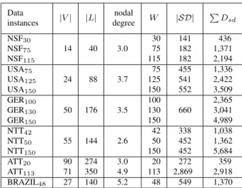
For the sake of comparison, we use the same data set as in [Jaumard and Daryalal,2017]. It involves six real network topologies: NSFNET, USANET, GERMANY, NTT, ATT, and BRAZIL (see AppendixD). Table2.1displays a summary of their characteristics: number of nodes and links, nodal degree, number of available wavelengths (i.e., transport capacity), number of node-pairs with

(25)

traffic, overall demand. The traffic instances have been generated randomly. For more details on the data set references, see [Jaumard and Daryalal,2017].

Table 2.1: Characteristics of the Datasets

Data _|_V_| _|_L_| nodal _W _|SD| P Dsd instances degree NSF30 14 40 3.0 30 141 436 NSF75 75 182 1,371 NSF115 115 182 2,194 USA75 24 88 3.7 75 455 1,336 USA125 125 541 2,422 USA150 150 552 3,509 GER100 50 176 3.5 100 660 2,365 GER130 130 3,041 GER150 150 4,989 NTT42 55 144 2.6 42 338 1,038 NTT50 50 452 1,362 NTT150 150 452 5,684 ATT20 90 274 3.0 20 272 359 ATT113 71 350 4.9 113 2,869 2,918 BRAZIL48 27 140 5.2 48 549 1,370

2.4.2 Efficiency of the L_CG model and algorithm

The newly proposed L_CG algorithm, described in Section2.3, was implemented and tested on a 3.6-4.0 GHz 4-cores machine with 32 GB RAM, using IBM[2016a] for the solution of the (integer) linear programs. Shortest path calculation was done with an open-source Java library JGraphT [Naveh,2016] implementing Dijkstra’s algorithm.

When computing the ILP solution of the last RMP, we observe that CPLEXcan take exceedingly longer time without adding much to the accuracy of the integral solution. Therefore, in order to achieve a better trade-off between the solution accuracy and the computational time, we used the following values for the CPLEXparameters (see [IBM,2016b] for more details on these parameters):

• Relative MIP gap tolerance =10−2 instead of the default CPLEX10−4value.

• Deterministic Time Limit = 200,000 ticks1. We are using a time limit in terms of the number of CPU ticks rather than in seconds in order to have a deterministic behavior across differ-ent hardware (server/computer) configurations. Only one instance (ATT20) actually reaches

1_{Deterministic Time Limit a computer-independent metric introduced by IBM. It measures how much algorithmic}

(26)

Table 2.2: Computational comparisons

Solution accuracies Computational performances (seconds)

Data L_CG ε(%) comparative L_CG Overall CPU comparative

sets z?

LP z˜ILP GoS (%) L_CG W_CG # cols

CPU L_CG W_CG Ratio LP ILP NSF30 430 429 98.4 0.2 2.1 600 0.8 0.1 0.9 9 10 NSF75 1,242 1,233 89.8 0.7 1.0 1,673 2.0 0.3 2.4 10 4.2 NSF115 1,924 1,922 87.6 0.1 0.8 2,104 3.4 0.3 3.7 10 2.7 USA75 1,281 1,275 95.4 0.5 3.1 1,532 5.6 0.2 5.8 141 24.3 USA125 2,255 2,239 92.4 0.7 2.4 4,099 26.3 20.0 46.6 155 3.3 USA150 3,029 3,008 85.7 0.7 1.8 3,460 28.2 0.6 29.0 176 6.1 GER100 2,306 2,277 96.3 1.3 2.7 3,576 51.7 52.0 103.9 474 4.6 GER130 2,960 2,928 96.3 1.1 2.4 4,520 86.0 44.1 130.3 521 4.0 GER150 4,663 4,611 81.4 1.1 3.1 6,054 248.7 23.4 272.4 1,817 6.7 NTT42 1,038 1,037 99.9 0.1 0.0 1,096 0.7 0.1 0.9 30 33.3 NTT50 1,362 1,356 99.6 0.4 0.0 1,415 1.2 0.0 1.3 37 28.5 NTT150 5,553 5,507 96.9 0.8 0.9 5,878 14.3 0.1 14.5 231 15.9 ATT20 359 347 96.7 3.5 1.4 1,065 2.7 286.6 289.4 1,549 5.4 ATT113 2,918 2,890 99.0 1.0 0.5 4,461 342.3 119.5 462.0 1,597 3.5 Brazil48 1,370 1,358 99.1 0.9 3.9 2,199 4.5 9.2 13.8 586 42.5 Average 0.9 1.7 91.8 489 5.3

that limit. Hence, our parameter selection helps to mitigate the effect of this particular data instance on the overall performance of the L_CG algorithm.

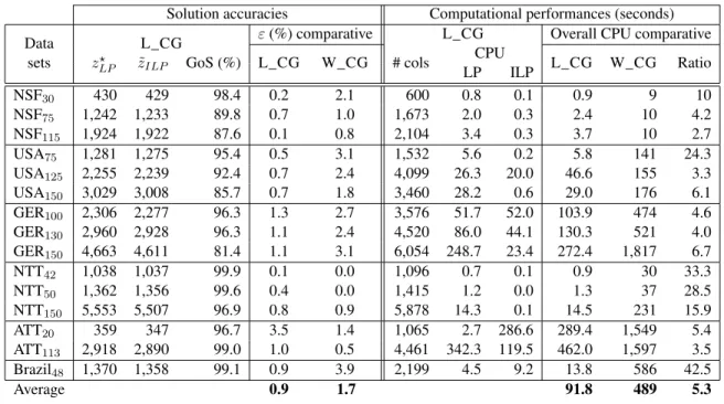
Comparative results are presented in Table 2.2. In the first part of Table 2.2, we provide the lower and upper bounds (z_LP? andz˜ILP) output by the L_CG algorithm. As both algorithms solve

exactly the linear relaxations, the lower bounds they output are identical. However, as can be seen with their comparative accuracy, their ILP solution differ. Accuracy (ε) is measured by the relative difference between the lower bound provided by the optimal solution (z_LP? ) of the linear relaxation of the Master Problem (PM), and the upper bound derived from the value of the ILP solution (z˜ILP),

see formula (2.5).

We observe that the L_CG algorithm outputs RWA provisioning with a higher accuracy than the W_CG algorithm, down from an average ofε= 1.7to less than 1%.

In the second part of Table2.2, we compare the computational times. We observe that the L_CG algorithm is faster than the W_CG algorithm: from 3 to 42 times faster, for an average of 5 times faster.

(27)

Figure 2.3: Characteristics of the Selected Lightpaths

scalable than the prior study, and is capable of finding better integral solutions with a smaller accu-racy gap.

2.4.3 Percentage of Shortest Paths in the Optimal RWA Provisioning

In order for an algorithm to find a near optimal solution, it must be able not only to consider all the shortest paths for any given node pair, but also to find the lightpaths that do not necessarily correspond to shortest paths. On the other hand, the intuition dictates that, in general, the use of lightpaths longer than shortest paths restrains the capability of provisioning other connections. Consequently, the algorithm must also use the shortest paths as much as possible.

In Figure 2.3, we provide the distribution of the selected lightpaths in terms of their lengths in the optimal RWA provisioning, as output by the L_CG algorithm. The columns of the chart correspond to the length of the routing paths used by the selected connections in unit of number of hops (e.g., SP+1 represents the number of connections routed on a path that is one hop longer than the shortest path of the corresponding node-pair).

We can observe that the solutions output by the L_CG model and algorithm contain a large fraction of shortest paths. Indeed, the average percentage of usage of shortest paths among all the

(28)

model and algorithm, i.e., 66%.

Taking into account that the accuracy of the solutions is less than 1% for nearly all of them, it is unlikely that the percentage of shortest paths would be able to decrease much more.

These improvements were obtained using a modeling that bear some symmetry and require more variables (columns) than the W_CG model, i.e., around at least |V|2 _{× |}_Λ_|_{columns (or in} other words, at least one lightpath per node pair with traffic and wavelength), while the W_CG model requires only at most |Λ| variables with non zero values. Indeed, the extra time that is potentially required for solving larger LPs is counterbalanced by the polynomial-time solution of the pricing problems, again even if there is a large number of them.

2.5 Conclusion

We proposed a very simple yet very efficient column generation decomposition to RWA problem using a lightpath-based decomposition model. Routes are dynamically generated using a weighted shortest path algorithm, where weights are determined by the values of the dual variables of the RMP, and take implicitly into account both the network connectivity and the traffic distribution.

Performances of the proposed decomposition schemes are compared with the best previously proposedε-optimal algorithm. Resulting accuracy values are on average less than 1%, down from 1.7% in [Jaumard and Daryalal,2017], and 5 times faster on average.

Additionally, we showcased that model symmetry is not a hindrance to its efficiency, although it may affect the performance of the branch-and-bound when deriving an ILP solution.

Future work will investigate the re-use of such a decomposition scheme for RSA networks, with preliminary promising results in [Enoch and Jaumard,2018b].

(29)

Chapter 3

Towards Optimal and Scalable Solution

for

Routing and Spectrum Allocation

Enoch and Jaumard[2018b]. Towards optimal and scalable solution for routing and spectrum allocation. Electronic Notes in Discrete Mathematics, 64, 335 - 344. 8th International Network Optimization Conference - INOC 2017.

3.1 Introduction

In order to face the steady growth of the optical networks, network operators are now moving to flexible or elastic optical networking. Therein, the optical spectrum is used more efficiently by allowing finer grid spacing, resulting in sub-streams, called slots. The challenge is then to optimize the spectrum usage through the so-called Routing and Spectrum Assignment (RSA) problem. It appears to be a much more difficult problem than the classical routing and wavelength assignment problem.

The paper is organized as follows. In Section3.2, after a detailed statement of the RSA problem, we describe the new decomposition model we propose. The solution scheme follows in Section3.3. Numerical results are described in Section3.4. Conclusions are drawn in the last section.

(30)

3.2 A New RSA Decomposition Model

3.2.1 Statement of the RSA Problem

The RSA problem assumes an undirected graphG = (V, L)with optical node set V and link setL. We denote byω(v)the set of links adjacent tov, forv∈V. The bandwidth is slotted into a setSof spectrum slots, and a guard band of one slot is required between spectrum slices assigned to different requests. The traffic is defined by a setK of requests where each requestk ∈Khas a source (sk), a destination (dk) and a spectrum demandDk, expressed in terms of a number of slots.

The traffic is assumed to be symmetrical.

3.2.2 RSA Decomposition Model

We propose a column generation model relying on lightpaths, where a lightpath, denoted byc, refers to the provisioning of a request using a routing path and a spectrum slice characterized by a starting slot denoted bys. LetCbe the set of all possible lightpaths. Each lightpath is characterized by:

• ac_k: indicates if a requestkis provisioned by lightpathc.

• bsc_` : indicates if a slotsis used on link`in lightpathc.

The model uses decision variableszcsuch that eachzcindicates if lightpathcis selected in the

solution.

The objective maximizes the throughput and is written:

z = max X c∈C X k∈K Dkack ! zc (3.1)

(31)

subject to: X c∈C ac_kzc≤1 k∈K (3.2) X c∈C bsc_` zc≤1 `∈L, s∈S (3.3) zc∈ {0,1} c∈C. (3.4)

Constraints (3.2) express that each request is provisioned at most once. Constraints (3.3) make sure that each slot is never used more than once on each fiber link.

3.3 Solution Design

Given the large number of variables/columns in the proposed model, we resort to theColumn Generationmethod to solve its Linear Programming (LP) relaxation [Chvatal,1983]. This technique consists of decomposing the original problem into a restricted master problem - RMP - (i.e., model (3.1) - (3.4) with a very restricted number of variables) and one or several pricing problem(s) - PP. RMP and PPs are solved alternately. Solving RMP consists in selecting the best lightpaths, while solving one PP allows the generation of an improving potential lightpath, i.e., a lightpath such that, if added to the current RMP, improves the optimal value of its LP relaxation. The process continues until the optimality condition is satisfied, that is, the so-called reduced cost that defines the objective function of the pricing problems is negative for all of them, see [Chvatal,1983] if not familiar with linear programming concepts. Anε-optimal solution for the RSA problem is derived by solving exactly the ILP model associated with the last RMP.

LetKsdenote the set of requests that have the potential to be provisioned by a lightpath which

starts at slots: Ks = {k ∈ K : s+Dk−1 ≤ |S|}.LetDsk be the number of slots needed for

(32)

D_ks=Dk k∈Ks : s+Dk−1 =|S| (3.5)

D_ks=Dk+ 1 k∈Ks : s+Dk−1<|S|. (3.6)

Each pricing problem is indexed bykands, and produces a single potential lightpath for provi-sioning demandk, starting at slots.

The definition of the decision variables is as follows:

• β`indicates if the lightpath uses link`or not ;

• bs_`0 indicates if slots0 is used on a link`or not.

Letµ(3.2)_k andµ(3.3)_`s0 be the values of the dual variables associated with constraints (3.2) and (3.3), respectively. The pricing problem can be written as follows:

rc = max Dk−µ(3.2)_k − X `∈L X s0_∈_S µ(3.3)_`s0 bs 0 ` (3.7) subject to: X `∈ω(sk) β` = X `∈ω(dk) β` = 1 (3.8) X `∈ω(v) β` ≤2 v∈V \ {sk, dk} (3.9) X `0_∈_ω₍_v₎_\{_`_} β`0 ≥β_` v∈V \ {s_k, d_k}, `∈ω(v) (3.10) s+Ds k−1 X s0₌_s bs_`0 =Ds_kβ` `∈L (3.11) β`, bs 0 ` ∈ {0,1} `∈L, s 0_∈_S (3.12)

Constraints (3.8), (3.9) and (3.10) define the routing of the current request. Constraints (3.11) reserve a contiguous spectrum channel for the current request.

(33)

bs_`0 =β` s0 ∈ {s, . . . , s+Dks−1}; (3.13)

bs_`0 = 0 s0 ∈ {/ s, . . . , s+D_ks−1}. (3.14)

Therefore, the reduced cost can be rewritten:

rc = max Dk−µ(3.2)_k − X `∈L   s+Ds k−1 X s0₌_s µ(3.3)_`s0  β`. (3.15)

The first term is a constant for each request, and the second term corresponds to a summation over the links of the network. Therefore, we can solve the pricing problem using the following objective function: min X `∈L   s+Ds k−1 X s0₌_s µ(3.3)_`s0  β`, (3.16)

whereµ(3.3)_`s0 are non-negative dual values. We conclude that, for each requestk, the lightpath gen-erator corresponds to a weighted shortest-path problem with link weight:

s+Ds k−1

P

s0₌_s

µ(3.3)_`s0 . As a result, the pricing problem can be solved with a polynomial time algorithm, e.g., Dijkstra’s algorithm.

The idea of using a shortest path algorithm during the pricing phase has been used by Ruiz et al.[2013a], but in our solution scheme, we solve exactly the LP relaxation of model (3.1) - (3.4) whereasRuiz et al.[2013a] do not.

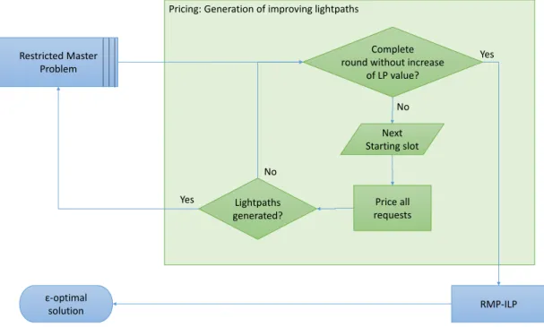
The flowchart of the solution process is depicted in Figure3.1. We reach the optimal LP solu-tion as soon as the LP optimality condisolu-tion is satisfied, i.e., we get a complete round of iterasolu-tions spanning all starting slots and all requests without any new improvement in the LP value.

We have noticed that this approach produces a large number of lightpaths that end up in the ILP problem, which can make the ILP solution process very long. In order to alleviate this problem, we followed an academic way of implementing column generation, which consists of removing the non basic columns, i.e., with variables which are equal to zero in the current LP solution after each optimization of the RMP. This technique allows a great speedup both during the column generation and the ILP solution phases.

(34)

RMP-ILP Price all requests ε-optimal solution Restricted Master Problem Yes No Next Starting slot Lightpaths generated?

Pricing: Generation of improving lightpaths

Complete round without increase

of LP value? No

Yes

Figure 3.1: Flow chart of the L_CG for RSA

3.4 Numerical Results

The model and solution design described above was implemented on a 3.6-4.0 GHz 4-cores machine with 32 GB of RAM, with the use of CPLEX (version 12.6.0) for solving the (integer) linear programs. Shortest path calculation was done with an open-source java library JGraphT implementing Dijkstra’s algorithm.

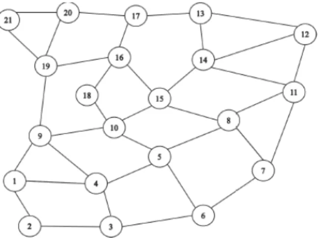
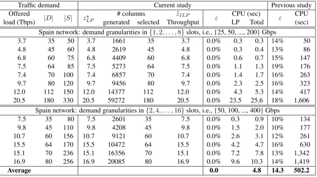
In a first set of experiments, we conducted experiments in order to assess the scalability of our solution process, and the accuracy of the RSA solutions that were output. We used the same set of data instances as [Jaumard and Daryalal, 2016], i.e., the Spain network with 21 nodes and 35 links (Figure3.2), the same demand sets, and the same spectral efficiency of 25 Gbps per slot. With regard to the criterion for removing less promising columns during the LP phase, and considering that these instances are relatively small, and therefore relatively easy to solve, we used a non-aggressive strategy consisting of removing columns with negative reduced price (within a small tolerance). Results are shown in Table3.1, and include a comparison with those of Jaumard and Daryalal[2016].

(35)

Figure 3.2: Spain network topology

observe also that our new model/algorithm is much faster, up to 2 orders of magnitude, and is capa-ble of finding the optimal RSA solutions, while all solution accuracies for the model and algorithm ofJaumard and Daryalal[2016] are larger than 10%.

In a second set of experiments, we use larger data sets: First series of data sets uses again the Spain network; Second series of data sets uses USA Network with 24 nodes and 43 links. In addition, these data sets have the following characteristics:

• Demands are drawn from granularities {4, 8, 16} with respective proportions {70%, 20%, 10%}, thus representing demands that are more representative of those encountered in today’s networks.

• Offered load is spread over all node pairs; Therefore, after aggregation, the number of requests given as input to our algorithm corresponds to the number of node pairs in the network. This means that number of aggregated requests is maximal, and that the size of the network is actually an accurate indicator of the size of the RSA problem instance.

Considering that these data sets are relatively large, we modified some of the execution param-eters to get the best performance as follows:

• During the LP phase, the least interesting columns are removed based on whether they are in the basis or not, and not based on the value of their reduced cost.

(36)

Traffic demand Current study Previous study

Offered _|

D| |S| z? LP

# columns ˜zILP

ε CPU (sec) ε CPU

load (Tbps) generated selected Throughput LP Total (sec)

Spain network: demand granularities in{1,2, . . . ,8}slots, i.e., {25, 50, ..., 200} Gbps

3.7 35 50 3.7 1661 35 3.7 0.0% 0.3 0.3 14% 50 4.8 45 60 4.8 2619 45 4.8 0.0% 0.3 0.4 13% 86 6.8 60 75 6.8 4409 60 6.8 0.0% 0.6 0.7 15% 147 7.5 64 85 7.5 5273 64 7.5 0.0% 1.1 1.3 19% 176 7.4 70 100 7.4 6857 70 7.4 0.0% 1.4 1.7 16% 263 9.7 80 120 9.7 9456 80 9.7 0.0% 2.3 2.5 16% 323 12.0 112 150 12.0 14377 112 12.0 0.0% 4.3 5.3 14% 417 20.5 180 330 20.5 59272 180 20.5 0.0% 23.5 25.6 18% 1,606

Spain network: demand granularities in{2,4, . . . ,16}slots, i.e., {50, 100, ..., 400} Gbps

7.5 35 80 7.5 2601 35 7.5 0.0% 0.3 0.9 10% 134 9.8 45 110 9.8 4208 45 9.8 0.0% 1.5 2.0 10% 177 10.7 60 156 10.7 9121 60 10.7 0.0% 2.6 3.1 12% 261 15.5 64 170 15.5 10472 64 15.5 0.0% 4.2 4.7 16% 630 15.1 70 236 15.1 16356 70 15.1 0.0% 7.2 7.8 13% 1,342 16.9 80 256 16.9 20085 80 16.9 0.0% 9.6 10.3 14% 1,419 Average 0.0 4.8 14.3 502.2

Table 3.1: Comparative Model/Algorithm Performance

from CPLEX, although it entails larger computational times.

• For the largest of these data sets, the number of columns in the ILP phase can be very large causing the ILP solver to run out of memory. To work around this issue, we apply a rounding technique where we remove the columns with the smallest values in the LP optimal solution (less than 0.2). This also improves the speed of the ILP phase while slightly sacrificing on the quality of the solution.

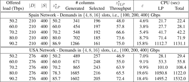
The summary of these experiments is shown in Table 3.2. Even for the larger network USA, and with large offered loads (up to 70 Tbps), the gap between the linear solution and the integral solution remains small, and only for the largest data sets does the gap become greater than 10%. More remarkably, the time of execution for most of the data sets is within seconds, and only for the largest data sets does the time become in the order of minutes, and in any case, less than 30 minutes, which is much faster than any previous work with comparable datasets.

Indeed, instances with an upper bound (z_LP? ) that differs from the offered load appear to be more difficult to solve. They require significantly more computational time, and the accuracy of the ILP solution decreases.

(37)

Offered

|D| |S| z?_LP # columns z

?

ILP _ε CPU (sec)

load (Tbps) Generated Selected Throughput LP Total

Spain Network - Demands in{4,8,16}slots, i.e., {100, 200, 400} Gbps

50.2 210 400 50.2 341 196 48.0 4.6% 21.7 22.4

60.0 210 400 60.0 454 197 57.8 3.8% 27.7 28.1

70.2 210 400 70.2 548 192 66.6 5.4% 41.7 42.2

80.0 210 400 80.0 702 185 73.6 8.7% 71.4 71.9

90.2 210 400 86.9 1266 161 75.0 15.8% 1112.7 1131.1

USA Network - Demands in{4,8,16}slots, i.e., {100, 200, 400} Gbps

50.2 276 400 50.2 489 257 46.9 7.0% 28.1 29.4

60.0 276 400 60.0 671 248 55.0 9.1% 53.3 55.8

70.2 276 400 70.2 865 243 63.9 9.9% 101.0 108.4

80.0 276 400 78.3 1685 216 65.5 19.6% 1050.8 1122.0

90.2 276 400 85.7 1602 205 72.4 18.4% 1495.2 1532.0

Table 3.2: Numerical results for new datasets

3.5 Conclusions

In this work, we proposed a new column generation model and algorithm for solving the RSA problem. In doing so, we defined a decomposition based on starting slots and on requests in such a way that the pricing problem was reduced to a shortest path problem, thus improving greatly the performance and improving significantly the accuracy of the RSA solutions that are output. As a result, we achieved a performance that is clearly better than the previous works.

However, further investigations on alternate models are needed. With the proposed model, for larger data sets with, e.g., 100 nodes or more, the number of columns in the ILP phase will be too large. Although the key for getting better ILP solutions than in the literature for this study, such a large number of columns is a bottleneck for solving the RSA problem with larger data sets.

(38)

Chapter 4

Nested Column Generation Algorithm

for the RWA Problem

In our previous RWA algorithm [Enoch and Jaumard,2018a], we proposed aLightpath decom-position model and solved it using Column Generationtechnique which resulted in considerable improvements over the earlier study [Jaumard and Daryalal,2017]. In this chapter, we consider the wavelengthConfigurationdecomposition model that was used in [Jaumard and Daryalal,2017], and we solve it using aNested Column Generationalgorithm.

4.1 Decomposition model

Given a WDM optical network, using the fixed frequency grid definition (i.e., the optical spec-trum is sliced into a number of wavelengths), and given a connection demand matrix, the RWA problem consists of allocating a routing path and an optical wavelength to each connection, as to maximize the Grade-of-Service (i.e., the proportion of granted connections).

A WDM optical network is represented by a directed graph G = (V, L) whereV represents the nodes of the network, andLis the set of links representing the directional optical fibers. The optical spectrum is divided into a set of wavelengths with equal capacity (50 GHz), denoted byΛ. LetW =|Λ|. The traffic is defined by a|V| × |V|matrix where each elementDsd represents the

(39)

node-pairs with traffic.

We propose an ILP model based on aConfigurationdecomposition. We define aConfiguration

as a set of link-disjoint lightpaths provisioning distinct connections on the same wavelength as illustrated in Figure4.1. Links are assumed to be bi-directional. Each link is used at most once in each direction.

Figure 4.1: RWA wavelengthConfiguration.

LetC be the set of all possibleConfigurations. EachConfigurationc ∈ C is defined with the help of the following parameter:

• ac

sd: gives the number of connections from vs tovd that are provisioned byConfiguration

c. Given that eachConfigurationis constructed on a single wavelength, this parameter cor-responds to the number of routing paths allocated for the given node pair on the current wavelength.

The model uses two sets of decision variables:

• zcis an integer variable that gives the number of occurrences ofConfigurationcin the

solu-tion.

• ysdis an intermediate integer variable that computes the number of granted connections from

vstovdin the solution, and can be expressed in terms ofzcas follows:

ysd =

X

(40)

The ILP model is the same as the one in [Jaumard and Daryalal,2017] and reads as follows: z = max X (vs,vd)∈SD ysd (4.2) subject to: X c∈C zc≤W (4.3) ysd ≤ X c∈C ac_sdzc (vs, vd)∈SD (4.4) ysd ≤Dsd (vs, vd)∈SD (4.5) zc∈N c∈C (4.6) ysd ≥0 (vs, vd)∈SD. (4.7)

Constraints (4.3) ensure that the acceptedConfigurationsare within the number of available wave-lengths. Constraints (4.4) ensure that the GoS calculated by the variablesysd is backed by actual

provisioning in theConfigurationszc. Constraints (4.5) limit the number of granted connections to

the demand.

In addition to this model (with two sets of variables), Jaumard and Daryalal [2017] provided another formulation not making use of the intermediate variables ysd (see Appendix C). In the

process of the current research, we investigated both models by implementing both of them using

Nested Column Generation. We have discovered that the one-variable-set formulation performs very poorly both in terms of the quality of the solution, and in terms of the computation time. The intuition behind this is that the Configurationcolumns are relatively large which makes LP relaxation take longer to converge to its optimal value (z?_LP). This also leads to a high contention among the Configurationsduring the ILP Branch-and-Bound phase, which produces an integral solution (z˜ILP) with a relatively large accuracy gap.

On the other hand, the two-variable-sets model uses a set of intermediate variables ysd which

(41)

constraints (4.4) are a relaxation of the definition (4.1). As a consequence of this relaxation, the two-variable-sets model requires to post-process theConfigurationsin the final solution, as to remove the extra provisioning that violates the demand constraints and to re-establish the equality (4.1).

In the sequel of this chapter we will describe the solution design for the two-variable-sets model which was used to produce the results in [Jaumard and Daryalal,2017] too.

4.2 Nested Column Generation

Column Generation consists of decomposing the original problem into a Restricted Master Problem(RMP), i.e., with a restricted number of variables, and one or severalPricing Problems

(PP). The RMP and the PP(s) are solved alternately. Solving the RMP consists in selecting the best columns, while solving one PP allows the generation of an improving potential column, i.e., a column such that, if added to the current RMP, improves the optimal value of its LP relaxation. The process continues until the optimality condition is satisfied, i.e., the so-called reduced cost that de-fines the objective function of thePricing Problemsis non-positive for all of them [Chvatal,1983]. The optimal value of the linear relaxation of the so-obtained RMP is denoted byz_LP? and represents an upper-bound on the optimal solution of the RWA problem. After theColumn Generationphase, the next step consists of solving the ILP model associated with the last RMP, which produces an integral solution with a value, denoted as z˜ILP, which represents a lower-bound on the optimal

solution of the RWA problem. The integral solution thus-obtained is said to beε-optimal whereε denotes the relative difference between the two bounds: ε= (z?_LP−z˜ILP)/zLP? .

Considering theConfigurationdecomposition in [Jaumard and Daryalal,2017], although Col-umn Generationis a powerful technique, we observed that the link-based formulation of thePricing Problemwas not efficient enough. Given that thePricing Problemsneed to be solved at each it-eration of Column Generation, their performance can be an important hindrance to the over-all efficiency. In order to address this difficulty, we devised an algorithm based on the idea of solv-ing thePricing Problemitself usingColumn Generation, which approach is referred to asNested Column Generation.

(42)

4.2.1 Review of Nested Decompositions

The idea of applying recursive decomposition was suggested byDantzig[1963]. Some of the first generic implementations forLinear Program (LP)go back to the early 70’s such asGlassey [1973] andHo and Manne[1974]. Subsequently, many implementations forInteger Linear Pro-graminghave been produced.

Vanderbeck[2001] implemented a nested decomposition approach to a cutting-stock problem. First the author devise a subproblem that generatescutting patternsand solves it usingColumn Gen-eration, in turn, with the help of another subproblem that generatessections. The author notes that the cutting-pattern generation subproblem is only solved approximately given thatColumn Gener-ationonly produces lower and upper bounds on the minimum reduced cost of a cutting-pattern, and uses the lower bounds on the reduced costs to produce a Lagrangian bound on the cutting problem. The author recognizes that this is a "heuristic based on the tools of exact optimization", given that the optimality of the Lagrangean bound is not guaranteed.

Hennig et al.[2012] proposed aNested Column Generationalgorithm for theCrude Oil Tanker Routing and Scheduling problem such that the first subproblem generates a cargo-route for each ship. This subproblem is solved using aBranch-and-Pricealgorithm with the help of a second-level subproblem which generates a route for each ship.

Closer to the applications in optical networks,Vignac et al.[2016] presented multiple models for theGrooming, Routing and Wavelength Assignmentproblem, among which, aColumn Generation

algorithm where a subproblem for each wavelength is defined to find the traffic carried by this wavelength, called aWavelength Routing Configuration. This subproblem is itself decomposed into arc-disjoint grooming-patterns, thus leading to a nested decomposition. Similarly to Vanderbeck [2001], the bounds of the Pricing Problemsare used to compute Lagrangean dual bounds on the master LP, thus resulting into a heuristic.

Caprara et al.[2016] referred toNested Column GenerationasRecursive Dantzig-Wolfe Refor-mulationand used this approach to design aBranch-and-Pricealgorithm for solving theTemporal Knapsack Problem.

(43)

Resource Interdependencies where both theMaster Problemand the Pricing Problem are solved using Branch-and-Price. The authors also give a detailed review on the use of nested decompositions in other publications (e.g.,Cordeau et al.[2001];Dohn and Mason[2013]).

4.2.2 Processing Flow

Figure 4.2: Nested Column Generation Flow for RWA

Figure4.2 shows the processing flow of ourNested Column Generation algorithm as applied to the RWA problem. TheColumn Generationflow used to solve the Pricing problem, is identical to that used to solve the Master problem, thus the naming ofNested Column Generation. We exit the process of generatingConfigurationsfor theMaster Problem, when thePricing Problemcannot produce an improvingConfiguration, i.e., the optimal value of the ILP associated with thePricing Problemis null (rc?

ILP = 0).

4.2.3 Optimality of the Linear Relaxation

The main outcome ofColumn Generationis to produce a strong linear relaxation boundz?_LP on the optimal solution of theMaster Problem. This outcome is based on the premise that thePricing Problemis solved to optimality [Dantzig,1963], in particular, when the stopping condition to exit

(44)

Column Generationis verified (rc?_ILP = 0). However, inNested Column Generation, thePricing Problemis solved usingColumn Generationmeaning that the integer solutions that we obtain for thePricing Problemsare only lower-bounds (assumingBranch-and-Priceis not employed as is the case in this study).

Nevertheless, thanks toNested Column Generation, we have also an upper bound on the optimal solution of the Pricing Problem (rc?

LP). So when the Pricing Problem fails to generate a new Configuration(rc˜ILP = 0), there are two possibilities:

• rc?_LP = 0: we can deduce thatrc?_ILP = 0, and therefore the exit condition is satisfied. In this case, the LP relaxation of theMaster Problemis optimal.

• rc?_LP >0: this means there is no guarantee thatrc?_ILP = 0, and therefore, the LP relaxation of theMaster Problemmight not be optimal.

To sum up, theoretically Nested Column Generation does not guarantee the accuracy of the LP relaxation bound of the Master Problem (). In fact, some studies resorted to a Branch-and-Price approach (with additional overhead) for solving the Pricing Problem in order to guarantee this accuracy [Hennig et al.,2012;Caprara et al.,2016;Tilk et al.,2018]. However, it is possible empirically to conclude whether the LP relaxation is optimal or not by verifying if the Pricing Problemwas solved to optimality in the last iteration.

4.3 Solution Design

As shown in Figure4.2, we applyNested Column Generationwhere we define aPricing Prob-lemthat feedsConfigurations to the Master Problem, and we solve this Pricing Problem in turn using Column Generation, meaning that we define a Nested Pricing Problem which feeds Light-pathsto the first levelPricing Problem.

4.3.1 Pricing Problem

The Pricing Problemaims to generate a Configurationcfor any wavelength. In the sequel of this section, we will drop thecindex to alleviate the mathematical notation.

(45)

Letµandµsd be the dual values corresponding to constraints (4.3) and (4.4) respectively. The

reduced cost corresponding to the model ((4.2)-(4.7)) is:

rc = max X

(vs,vd)∈SD

µsdasd − µ (4.8)

Generating aConfigurationconsists of finding routing pathsπfor connections between different node-pairs. LetΠsdbe the set of all possible paths fromvstovd. A routing path is defined with the

help of the following parameters:

• δ_π` is a binary parameter that indicates if link`is part of routing pathπ.

We define the following decision variables:

• βπ is a boolean variable that indicates if a pathπis selected in the currentConfiguration.

We can write the correspondence between βπ and the parameters of the Master Problem as

follows:

asd =

X

π∈Πsd

βπ (vs, vd)∈SD. (4.9)

After a variable substitution in the reduced cost (4.8), we obtain thePricing Problemmodel as follows: rc = max X (vs,vd)∈SD X π∈Πsd µsdβπ − µ (4.10) subject to: X π∈Πsd βπ ≤Dsd (vs, vd)∈SD (4.11) X (vs,vd)∈SD X π∈Πsd δ_π`βπ ≤1 `∈L (4.12) βπ ∈ {0,1} π ∈Π. (4.13)

(46)

Constraints (4.11) limit the number of paths for a given node-pair to the demand. Constraints (4.12) mean that each link is traversed by at most one path. This ensures that the paths forming the

Configurationare link-disjoint.

4.3.2 Path Generator

The path generator (Nested Pricing Problem) aims to generate routing paths for each node-pair, and feeds them to the - first level -Pricing Problem.

Let νsd andν` be the dual values corresponding to constraints (4.11) and (4.12) respectively.

For each node-pair(vs, vd)∈SD, the reduced cost of a pathπ ∈Πsd is:

max µsd−νsd−

X

`∈L

ν`δ`π. (4.14)

We get a shortest-path problem with non-negative weights for each(vs, vd)∈SD

min X

`∈L

ν`δπ` (4.15)

which is solved in polynomial time.

4.4 Numerical Results

We ran this algorithm on the same dataset as in [Jaumard and Daryalal,2017;Enoch and Jau-mard,2018a]. For the best performance, we ran CPLEX in a single thread and we turned on the

CPX_PARAM_NUMERICALEMPHASIS 1 switch. We have also observed that the ILP phase can take too long without adding much to the quality of the integral solution. Therefore we opted to pre-terminate the ILP phase by setting the parameterCPX_PARAM_EPGAP2to 1.e-1, thus making a trade-off in the benefit of computation time. Table4.1shows the complete results and comparison with the previous algorithms. (We did not re-implement the reference algorithm W_CG presented byJaumard and Daryalal[2017], and the results shown below are those published by its authors.)

1

Numerical precision emphasis

2

(47)

Table 4.1: W_NCG Algorithm Results and Comparison

Solution Computational performance (sec)

W_NCG (%) comparative W_NCG Overall CPU comparative

Data set z?

LP z˜ILP GoS (%) W_NCG L_CG W_CG # cols LP CPU ILP CPU W_NCG L_CG W_CG

NSF30 430 395 90.6 8.9 0.2 2.1 66 1.0 0.2 1.2 0.9 9 NSF75 1242 1205 87.8 3.1 0.7 1.0 71 1.2 0.1 1.3 2.4 10 NSF115 1924 1890 86.1 1.8 0.1 0.8 68 0.8 0.1 0.9 3.7 10 USA75 1281 1170 87.6 9.5 0.5 3.1 169 19.0 0.9 19.9 5.8 141 USA125 2255 2094 86.5 7.7 0.7 2.4 174 30.3 0.2 30.5 46.6 155 USA150 3029 2895 82.5 4.6 0.7 1.8 171 25.5 0.2 25.7 29.0 176 GER100 2306 2114 89.4 9.1 1.3 2.7 211 59.1 2.0 61.1 103.9 474 GER130 2960 2738 90.0 8.1 1.1 2.4 251 88.9 0.9 89.8 130.3 521 GER150 4663 4314 76.1 8.1 1.1 3.1 282 318.7 3.6 322.3 272.4 1817 NTT42 1038 1038 100.0 0.0 0.1 0.0 15 0.1 0.1 0.2 0.9 30 NTT50 1362 1341 98.5 1.6 0.4 0.0 36 0.4 0.1 0.5 1.3 37 NTT150 5553 5271 92.7 5.4 0.8 0.9 167 9.5 0.5 10.0 14.5 231 ATT20 359 322 89.7 11.5 3.5 1.4 90 5.4 0.4 5.8 289.4 1549 ATT113 2918 2897 99.3 0.7 1.0 0.5 627 216.7 1.6 218.3 462.0 1597 Brazil48 1370 1242 90.7 10.3 0.9 3.9 132 17.3 1.6 18.9 13.8 586 Average 6.0 0.9 1.7 53.8 91.8 490

We observe for all the instances that: When thePricing Problemfails to generate a new Config-uration(i.e.,rc˜ILP = 0), we have alsorc?_LP = 0, which implies thatrc?_ILP = 0meaning that the Pricing Problemis solved optimally. Therefore, the LP relaxation solution obtained for the Mas-ter Problemz?_LP is optimal and is an upper-bound on the optimal solutionz_ILP? (see discussion at Section4.2.3).

Due to the pre-termination of the ILP phase, the time spent in this phase is very small, which leads to an overall computation time of 53.8 seconds on average which is better than the other algorithms. However, the ILP gap of 6% on average is larger than the other algorithms. This can be partially due the large size of theConfigurationcolumns as compared to theLightpathcolumns. In fact, even if the number of columns in theConfigurationdecomposition is smaller, it intersects with more constraints which makes for an ILP with a higher density, thus more difficult to solve.

Although the W_NCG algorithm is fast, it suffers from a large accuracy gap of the integral solution. The algorithm L_CG presented in [Enoch and Jaumard,2018a] using aLightpath decom-position remains the best performing algorithm overall.

Advanced Column Generation Decompositions for Optimizing Provisioning Problems in Optical Networks