http://waikato.researchgateway.ac.nz/
Research Commons at the University of Waikato
Copyright Statement:
The digital copy of this thesis is protected by the Copyright Act 1994 (New Zealand).
The thesis may be consulted by you, provided you comply with the provisions of the Act and the following conditions of use:
Any use you make of these documents or images must be for research or private study purposes only, and you may not make them available to any other person.
Authors control the copyright of their thesis. You will recognise the author’s right to be identified as the author of the thesis, and due acknowledgement will be made to the author where appropriate.
You will obtain the author’s permission before publishing any material from the thesis.
Department of Computer Science
Hamilton, NewZealand
Best-first Decision Tree Learning
Haijian Shi
This thesis is submitted in partial fulfilment of the requirements for the degree of Master of Science at The University of Waikato.
2006 c
Abstract
Decision trees are potentially powerful predictors and explicitly represent the structure of a dataset. Standard decision tree learners such as C4.5 expand nodes in depth-first order (Quinlan, 1993), while in best-first decision tree learners the ”best” node is expanded first. The ”best” node is the node whose split leads to maximum reduction of impurity (e.g. Gini index or information in this thesis) among all nodes available for splitting. The resulting tree will be the same when fully grown, just the order in which it is built is different. In practice, some branches of a fully-expanded tree do not truly reflect the underlying information in the domain. This problem is known as overfitting and is mainly caused by noisy data. Pruning is necessary to avoid overfitting the training data, and discards those parts that are not predictive of future data. Best-first node expansion enables us to investigate new pruning techniques by determining the number of expansions performed based on cross-validation.
This thesis first introduces the algorithm for building binary best-first decision trees for classification problems. Then, it investigates two new pruning methods that determine an appropriate tree size by combining best-first decision tree growth with cross-validation-based selection of the number of expansions that are performed. One operates in a pre-pruning fashion and the other in a post-pruning fashion. They are called best-first-based pre-pruning and best-first-based post-pruning respectively in this thesis. Both of them use the same mechanisms and thus it is possible to compare the two on an even footing. Best-first-based pre-pruning stops splitting when further splitting increases the cross-validated error, while best-first-based post-pruning takes a fully-grown decision tree and then discards expansions based on the cross-validated error. Because the two new pruning methods implement cross-validation-based pruning, it is possible to compare the two to another cross-validation-based pruning method: minimal cost-complexity pruning (Breiman et al., 1984). The two main results are that best-first-based pre-pruning is competitive with best-first-based post-pruning if the so-called ”one standard error rule” is used. However, minimal
cost-complexity pruning is preferable to both methods because it generates smaller trees with similar accuracy.
Acknowledgments
This thesis would not have been possible without the support and assistance of the people in the Department of Computer Science at the University of Waikato, especially the members of machine learning group. These people provides me a very good environment to do my research in New Zealand.
First and foremost, I would like to thank my supervisor Dr. Eibe Frank for guiding me through the whole thesis. He provided a lot of useful materials and helped with implementation problems I encountered during the development. He also helped me revise over the thesis draft. Moreover, he gave me valuable suggestions of how to run the experiments presented in this thesis.
Special thanks to Dr. Mark Hall who told me how to use the rpart package (the implementation of the CART system in the language R). This helped me do a comparison between my basic implementation of the CART system in Java and the rpart package in order to make sure that there is no problem in my implementation. I would also like to thank all members in the machine learning group. I gained so much useful knowledge from the weekly meetings and e-mails sent to me. These guys are so friendly and helped me solve many problems I met.
Contents
Abstract i Acknowledgments iii List of Figures ix List of Tables xi 1 Introduction 11.1 Basic concepts of machine learning . . . 1
1.2 Decision trees . . . 2
1.2.1 Standard decision trees . . . 3
1.2.2 Best-first decision trees . . . 3
1.3 Pruning in decision trees . . . 5
1.4 Motivation and objectives . . . 6
1.5 Thesis structure . . . 7
2 Background 9 2.1 Pruning methods related to cross-validation . . . 9
2.1.1 Minimal cost-complexity pruning . . . 10
2.1.2 Other pruning methods related to cross-validation . . . 16
2.2 Pruning in standard decision trees . . . 18
2.2.1 Pre-pruning and post-pruning . . . 19
2.2.2 Comparisons of pre-pruning and post-pruning . . . 20
2.3 Best-first decision trees in boosting . . . 21
2.4 Summary . . . 23
3 Best-first decision tree learning 25 3.1 Splitting criteria . . . 27
3.1.1 Information . . . 29
3.1.2 Gini index . . . 30
3.2.1 Numeric attributes . . . 33
3.2.2 Nominal attributes . . . 35
3.2.3 The selection of attributes . . . 39
3.3 Best-first decision trees . . . 41
3.3.1 The best-first decision tree learning algorithm . . . 42
3.3.2 Missing values . . . 44
3.4 Pruning . . . 45
3.4.1 Best-first-based pre-pruning . . . 46
3.4.2 Best-first-based post-pruning . . . 48
3.4.3 The 1SE rule in best-first-based pre-pruning and post-pruning 49 3.5 Complexity of best-first decision tree induction . . . 51
3.6 Summary . . . 52
4 Experiments 55 4.1 Datasets and methodology . . . 55
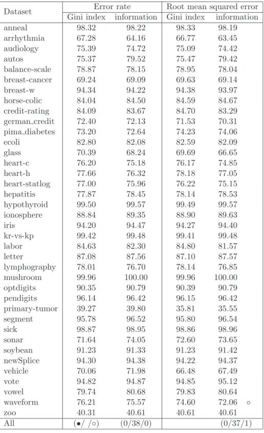
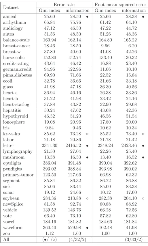
4.2 Gini index versus information . . . 58
4.3 Error rate versus root mean squared error . . . 62
4.4 Heuristic search versus exhaustive search . . . 66
4.5 The effects of the 1 SE rule in best-first-based pre-pruning and post-pruning . . . 68
4.5.1 Accuracy . . . 69
4.5.2 Tree size . . . 69
4.5.3 Discussion . . . 72
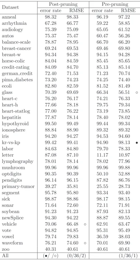
4.6 Comparing best-first-based pre-pruning and post-pruning . . . 72
4.6.1 Accuracy . . . 72
4.6.2 Tree size . . . 74
4.6.3 Training time . . . 74
4.6.4 Discussion . . . 76
4.7 Comparing best-first-based pre-pruning and post-pruning to minimal cost-complexity pruning . . . 78
4.7.1 Accuracy . . . 78
4.7.2 Tree size . . . 79
4.7.3 Training time . . . 82
4.8 The effects of training set size on tree complexity for best-first-based pre-pruning and post-pruning . . . 84 4.9 Summary . . . 87
5 Conclusions 91
5.1 Summary and conclusions . . . 91 5.2 Future work . . . 93
Appendices 95
A Possible binary splits on the attribute temperature 95 B Accuracy and tree size of pre-pruning and post-pruning for different
List of Figures
1.1 Decision trees: (a) a hypothetical depth-first decision tree, (b) a
hypo-thetical best-first decision tree. . . 4
2.1 (a) The treeT, (b) a branch ofT Tt5, (c) the pruned subtreeT ′ =T−T t5. 10 2.2 The tree for the parity problem. . . 21
3.1 The best-first decision tree on theiris dataset. . . 26
3.2 (a) The fully-expanded best-first decision tree; (b) the fully-expanded standard decision tree; (c) the best-first decision tree with three ex-pansions from (a); (d) the standard decision tree with three exex-pansions from (b). . . 27
3.3 Possible splits for the four attributes of the weather dataset. . . 30
3.4 The information value and the Gini index in a two-class problem. . . . 31
3.5 Possible binary splits on the attributetemperature. . . 34
3.6 Possible binary splits on the attributeoutlook. . . 36
3.7 The best-first decision tree learning algorithm. . . 43
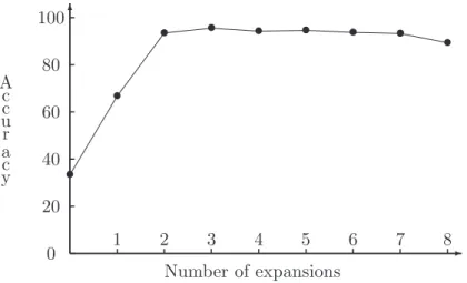
3.8 The accuracy for each number of expansions of best-first decision tree learning on the iris dataset. . . 45
3.9 The best-first-based pre-pruning algorithm. . . 47
3.10 The best-first-based post-pruning algorithm. . . 49
List of Tables
2.1 The sequence of pruned subtrees from T1, accompanied by their
corre-sponding α values on the balance-scale dataset. . . 12 2.2 Rcv(Tk) for different seeds without 1SE on thebalance-scale dataset. . 14
2.3 Rcv(T
k) for different seeds with 1SE on the balance-scale dataset. . . . 15
2.4 A parity problem. . . 20 3.1 The instances of the weather dataset. . . 28 3.2 The class frequencies for the artificial attribute A. . . 38 3.3 Splitting subsets and their corresponding Gini gains and information
gains on the artificial attribute A. . . 40 3.4 The error rate and the root mean squared error for each expansion using
best-first decision tree learning on theglass dataset. . . 48 3.5 The error rate and the root mean squared error for each expansion with
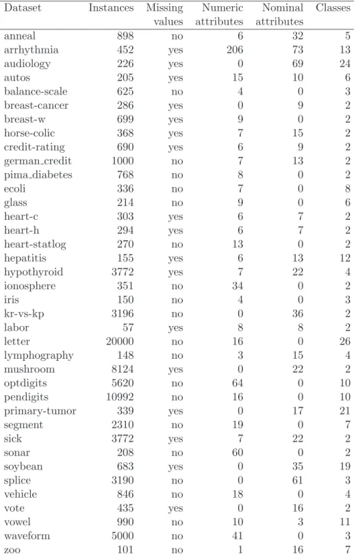
1SE using best-first decision tree learning on the glass dataset. . . 50 4.1 The 38 UCI datasets and their properties. . . 57 4.2 The accuracy of best-first-based post-pruning using (a) the Gini index
and (b) the information. . . 60 4.3 The tree size of best-first-based post-pruning using (a) the Gini index
and (b) the information. . . 61 4.4 The accuracy of best-first-based pre-pruning and post-pruning using
(a) the error rate and (b) the root mean squared error. . . 64 4.5 The tree size of best-first-based pre-pruning and post-pruning using (a)
the error rate and (b) the root mean squared error. . . 65 4.6 The multi-class datasets used for comparing heuristic search and
ex-haustive search. . . 67 4.7 The accuracy for heuristic search and exhaustive search. . . 68 4.8 The accuracy for heuristic search and exhaustive search on three
datasets whose attribute with maximum number of values has been deleted. . . 68
4.9 The accuracy of best-first-based pre-pruning and post-pruning both with and without the 1SE rule. . . 70 4.10 The tree size of best-first-based pre-pruning and post-pruning both with
and without the 1SE rule. . . 71 4.11 Comparing the accuracy of best-first-based pre-pruning and
post-pruning (both with and without the 1SE rule). . . 73 4.12 Comparing the tree size of best-first-based pre-pruning and
post-pruning (both with and without the 1SE rule). . . 75 4.13 Comparing the training time of best-first-based pre-pruning and
post-pruning (both with and without the 1SE rule). . . 77 4.14 Comparing the accuracy of the two new pruning methods and minimal
cost-complexity pruning (both with and without the 1SE rule). . . 80 4.15 Comparing the tree size of the two new pruning methods and minimal
cost-complexity pruning (both with and without the 1SE rule). . . 81 4.16 Comparing the training time of the two new pruning methods and
min-imal cost-complexity pruning (both with and without the 1SE rule). . 83 4.17 The accuracy and tree size of best-first-based pre-pruning on different
training set sizes (both with and without the new 1SE rule). . . 85 4.18 The accuracy and tree size of best-first-based post-pruning for different
training set sizes (both with and without the new 1SE rule). . . 85 4.19 The effect of random data reduction on tree complexity for
best-first-based pre-pruning (both with and without the new 1SE rule). . . 86 4.20 The effect of random data reduction on tree complexity for
best-first-based post-pruning (both with and without the new 1SE rule). . . 87 B.1 The accuracy of best-first-based pre-pruning without the new 1SE rule
for different training set sizes. . . 97 B.2 The tree size of best-first-based pre-pruning without the new 1SE rule
for different training set sizes. . . 98 B.3 The accuracy of best-first-based pre-pruning with the new 1SE rule for
different training set sizes. . . 98 B.4 The tree size of best-first-based pre-pruning with the new 1SE rule for
different training set sizes. . . 99 B.5 The accuracy of best-first-based post-pruning without the 1SE rule on
B.6 The tree size of best-first-based post-pruning without the 1SE rule for different training set sizes. . . 100 B.7 The accuracy of best-first-based post-pruning with the 1SE rule for
different training set sizes. . . 100 B.8 The tree size of best-first-based post-pruning with the 1SE rule for
Chapter 1
Introduction
In the early 1990’s, the establishment of the Internet made large quantities of data to be stored electronically, which was a great innovation for information technology. However, the question is what to do with all this data. Data mining is the process of discovering useful information (i.e. patterns) underlying the data. Powerful techniques are needed to extract patterns from large data because traditional statistical tools are not efficient enough any more. Machine learning algorithms are a set of these techniques that use computer programs to automatically extract models representing patterns from data and then evaluate those models. This thesis investigates a machine learning technique called best-first decision tree learner. It evaluates the applicability of best-first decision tree learning on real-world data and compares it to standard decision tree learning.
The remainder of this chapter is structured as follows. Section 1.1 describes some basic concepts of machine learning which are helpful for understanding best-first decision tree learning. Section 1.2 discusses the basic ideas underlying best-best-first decision trees and compare them to standard decision trees. The pruning methods for best-first decision trees are presented briefly in Section 1.3. The motivation and objectives of this thesis are discussed in Section 1.4. Section 1.5 lists the structure of the rest of this thesis.
1.1
Basic concepts of machine learning
To achieve the goals of machine learning described above, we need to organise the input and output first. The input consists of the data used to build models. The input involves concepts,instances, attributes and datasets. The thing which is to be learnt is called the concept. According to Witten and Frank (2005), there are four different styles of concepts in machine learning, classification learning, association learning,
clustering and regression learning. Classification learning takes a set of classified examples (e.g. examples with class values) and uses them to build classification models. Then, it applies those models to classifying unseen examples. Association learning takes account of any association between features not just predicting class values. Clustering groups a set of similar examples together according to some criteria. Regression learning uses a numeric value instead of a class label for the class of each example.
The input of machine learning consists of a set of instances (e.g. rows, exam-ples or sometimes observations). Each instance is described by a fixed number of
attributes (i.e. columns), which are assumed to be either nominal or numeric, and a label which is calledclass (when the task is a classification task). The set of instances is called adataset. The output of machine learning is aconcept description. Popular types of concept descriptions are decision tables, decision trees, association rules, decision rules, regression trees and instance-based representations (Witten & Frank, 2005).
The four concepts described above can be organised into two categories, super-vised learning and unsupervised learning. Classification learning and regression learning are supervised learning algorithms. Insupervised classification learning, the induction algorithm first makes a model for a given set of labelled instances. Then, the algorithm applies the model to unclassified instances to make class predictions. In supervised regression learning, the induction algorithm maps each instance to a numeric value, not a class label. Association learning andclustering are unsupervised learning tasks that deal with discovering patterns for unlabelled instances. The best-first decision tree learner investigated in this thesis is a learning algorithm for
supervised classification learning.
1.2
Decision trees
A decision tree is a tree in which each internal node represents a choice between a number of alternatives, and each terminal node is marked by a classification. Decision trees are potentially powerful predictors and provide an explicit concept description for a dataset. In practice, decision tree learning is one of the most popular technique
in classification because it is fast and produces models with reasonable performance. In the context of this thesis there are two sorts of decision trees. One is constructed in depth-first order and called ”standard” decision tree. The other is constructed in best-first order and called ”best-first” decision tree. The latter type is the focus of this thesis.
1.2.1 Standard decision trees
Standard algorithms such as C4.5 (Quinlan, 1993) and CART (Breiman et al., 1984) for the top-down induction of decision trees expand nodes in depth-first order in each step using the divide-and-conquer strategy. Normally, at each node of a decision tree, testing only involves a single attribute and the attribute value is compared to a constant. The basic idea of standard decision trees is that, first, select an attribute to place at the root node and make some branches for this attribute based on some criteria (e.g. information or Gini index). Then, split training instances into subsets, one for each branch extending from the root node. The number of subsets is the same as the number of branches. Then, this step is repeated for a chosen branch, using only those instances that actually reach it. A fixed order is used to expand nodes (normally, left to right). If at any time all instances at a node have the same class label, which is known as a pure node, splitting stops and the node is made into a terminal node. This construction process continues until all nodes are pure. It is then followed by a pruning process to reduce overfittings (see Section 1.3).
1.2.2 Best-first decision trees
Another possibility, which so far appears to only have been evaluated in the context of boosting algorithms (Friedman et al., 2000), is to expand nodes in best-first order instead of a fixed order. This method adds the ”best” split node to the tree in each step. The ”best” node is the node that maximally reduces impurity among all nodes available for splitting (i.e. not labelled as terminal nodes). Although this results in the same fully-grown tree as standard depth-first expansion, it enables us to investigate new tree pruning methods that use cross-validation to select the number of expansions. Both pre-pruning and post-pruning can be performed in this way, which enables a fair comparison between them (see Section 1.3).
a. N
1
N2 N4
Leaf N3 Leaf Leaf
Leaf Leaf
b. N
1
N3 N2
Leaf N4 Leaf Leaf
Leaf Leaf
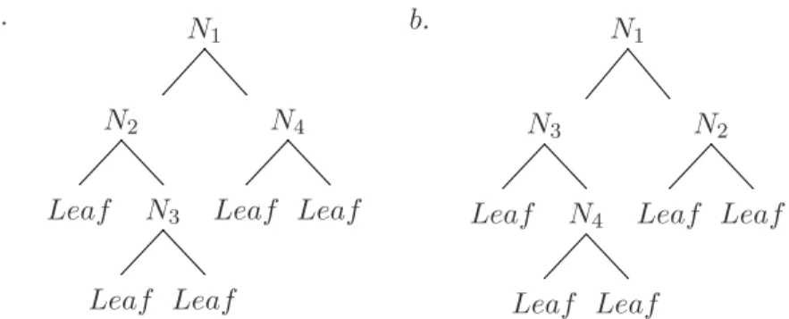
Figure 1.1: Decision trees: (a) a hypothetical depth-first decision tree, (b) a hypo-thetical best-first decision tree.
Best-first decision trees are constructed in a divide-and-conquer fashion similar to standard depth-first decision trees. The basic idea of how a best-first tree is built is as follows. First, select an attribute to place at the root node and make some branches for this attribute based on some criteria. Then, split training instances into subsets, one for each branch extending from the root node. In this thesis only binary decision trees are considered and thus the number of branches is exactly two. Then, this step is repeated for a chosen branch, using only those instances that actually reach it. In each step we choose the ”best” subset among all subsets that are available for expansions. This constructing process continues until all nodes are pure or a specific number of expansions is reached. Figure 1.1 shows the difference in split order between a hypothetical binary best-first tree and a hypothetical binary depth-first tree. Note that other orderings may be chosen for the best-first tree while the order is always the same in the depth-first case.
The problem in growing best-first decision trees is now how to determine which attribute to split on and how to split the data. Because the most important objective of decision trees is to seek accurate and small models, we try to find pure nodes as soon as possible. To measure purity, we can use its opposite, impurity. There are many criteria to measure node impurity. For example, the CART system (Breiman et al., 1984) uses Gini index and C4.5 (Quinlan, 1993) uses information. In this thesis, both the information and the Gini index are used to compare their different perfor-mance. The goal is to aim an attribute to split on that can maximally reduce impurity. Split selection methods used in this thesis are as follows. For a numeric at-tribute, the split is the same as that for most decision trees such as the CART system
(Breiman et al., 1984): the best split point is found and split is performed in a binary fashion. For example, a split on the iris dataset might be petallength < 3.5 and
petallength ≥ 3.5. For a nominal attribute, the node is also split into exactly two branches no matter how many values the splitting attribute has. This is also the same as the one used in the CART system. In this case, the objective is to find a set of attribute values which can maximally reduce impurity. Split methods are discussed in detail later in Chapter 3. For binary trees as the ones used in this thesis, it is obvious that each split step increases the number of terminal nodes by only one. The information and the Gini gain are also used to determine node order when expanding nodes in the best-first tree. The best-first method always chooses the node for expansion whose corresponding best split provides the best information gain or Gini gain among all unexpanded nodes in the tree.
1.3
Pruning in decision trees
Fully-expanded trees are sometimes not as good as smaller trees because of noise and variability in the data, which can result in overfitting. To prevent the problem and build a tree of the right size, a pruning process is necessary. In practice, almost all decision tree learners are accompanied by pruning algorithms. Generally speaking, there are two kinds of pruning methods, one that performs pre-pruning and another one that performs post-pruning. Pre-pruning involves trying to decide to stop splitting branches early when further expansion is not necessary. Post-pruning constructs a complete tree first and prunes it back afterwards based on some criteria. Pre-pruning seems attractive because it avoids expanding the full tree and throwing some branches away afterwards, which can save computation time, but post-pruning is considered preferable because of ”early stopping”: a significant effect may not be visible in the tree grown so far and pre-pruning may stop too early. However, empirical comparisons are rare.
Because all pruning procedures evaluated in this thesis are based on cross-validation, we now briefly explain how it works. In cross-cross-validation, a fixed number of folds is decided first. Assuming the number is ten, the data is separated into ten approximately equal partitions and each in turn is used for testing and the remainder
is used for training. Thus, every instance is used for testing exactly once. This is called ten-fold cross-validation. An error estimate is calculated on the test set for each fold and the ten resulting error estimates are averaged to get the overall error estimate. When pruning decision trees based on the methods investigated in this thesis, the final tree size is decided according to this average error estimate.
In the case of best-first decision trees, pre-pruning and post-pruning can be easily performed by selecting the number of expansions based on the error estimate by cross-validation, and this is what makes them different from standard decision trees. Here is the basic idea of how they work. For both pruning methods, the trees in all folds are constructed in parallel (e.g. ten trees for aten-fold cross-validation). For each number of expansion, the average error estimate is calculated based on the temporary trees in all folds. Pre-punning simply stops growing the trees when further splitting increases the average error estimate and chooses the previous number of expansion as the final number of expansions. Post-pruning continues expanding nodes until all the trees are fully expanded. Then it chooses the number of expansions whose average error estimate is minimal. In both cases the final tree is then built based on all the data and the chosen number of expansions.
This thesis compares the two new pruning methods to another cross-validation-based pruning method as implemented in the CART system, called ”minimal cost-complexity pruning” (Breiman et al., 1984). This pruning method is another kind of post-pruning technique. The basic idea of this pruning method is that it tries to first prune those branches that relative to their size which leads to the smallest increase in error on the training data. The details of minimal cost-complexity pruning are described in Chapter 2. The pre-pruning and post-pruning algorithms for best-first decision trees are described in Chapter 3.
1.4
Motivation and objectives
Significant research efforts have been invested into depth-first decision tree learners. Best-first decision tree learning has so far only been applied as the base learner in boosting (Friedman et al., 2000), and has not been paid too much attention in spite of the fact that it makes it possible to implement pre-pruning and post-pruning in
a very simple and elegant fashion, based on using the number of expansions as a parameter. Thus, this thesis investigates best-first decision tree learning. It investi-gates the effectiveness of pre-pruning and post-pruning using best-first decision trees. Best-first-based pre-pruning and post-pruning can be compared on an even footing as both of them are based on cross-validation. Minimal cost-complexity pruning is used as the benchmark pruning technique as it is also based on cross-validation and known to perform very well. As mentioned before, the best-first decision trees investigated in this thesis are binary, and the searching time of finding the optimum split for a nominal attribute using exhaustive search is exponential in the number of attribute values of this attribute, so we need to seek an efficient splitting method for nominal attributes. This thesis also lists two efficient search methods for finding binary splits on nominal attributes. One is for two-class problems (Breiman et al., 1984) and the other (i.e. heuristic search) is for multi-class problems (Coppersmith et al., 1999). In order to fulfil the tasks presented above, the objectives of this thesis are as follows:
1. To evaluate the applicability of best-first decision tree learning to real-world data.
2. To compare best-first-based pre-pruning and post-punning on an even footing using the best-first methodology.
3. To compare the two new best-first-based pruning algorithms to minimal cost-complexity pruning.
4. To compare heuristic search and exhaustive search for binary splits on nominal attributes in multi-class problems.
1.5
Thesis structure
To achieve the objectives described above, the rest of this thesis is organised in four chapters.
The background for the work presented in this thesis is described in Chapter 2. Some known pruning methods, related to cross-validation, are discussed first.
Minimal cost-complexity pruning is discussed in detail as it is involved in the experiments presented in this thesis. Other pruning methods are briefly described. Then, the principles of pre-pruning and post-pruning for standard decision trees are explained and compared. Finally, the paper that introduced best-first decision trees (Friedman et al., 2000), which applied best-first decision trees to boosting, is briefly described.
Chapter 3 discusses the best-first decision trees used in thesis in detail. It presents impurity criteria, splitting methods for attributes, error estimates to determine the number of expansions and the algorithm for constructing best-first decision trees. Pre-pruning and post-pruning algorithms for best-first decision trees are also described in this chapter. We discuss how the one standard error rule (i.e. the 1SE rule) can be used in these two pruning methods.
Chapter 4 provides the experimental results for 38 standard benchmark datasets from the UCI repository (Blake et al., 1998) for best-first decision tree learning presented in this thesis. We evaluate best-first-based pre-pruning and post-pruning using different splitting criteria and different error estimates (determine the number of expansions) to find which splitting criterion and error estimate is better. The performance of the two new pruning methods is compared in terms of classification accuracy, tree size and training time. Then, we compare their performance to minimal cost-complexity pruning in the same way. Experiments are also evaluated to see whether tree size obtained by best-first-based pre-pruning and post-pruning is influenced by training set size. Results for heuristic search and exhaustive search for finding binary splits on nominal attributes are also discussed.
Chapter 5 summarises material presented in this thesis, draws conclusions from the work and describes some possibilities for future work.
Chapter 2
Background
This chapter describes the background for the work presented in this thesis: pruning methods related to cross-validation, work on pre-pruning and post-pruning, and work on best-first decision trees in boosting. The chapter is structured as follows. Section 2.1 describes some known pruning methods related to cross-validation. Minimal cost-complexity pruning (Breiman et al., 1984) is described in detail because it is involved in the experiments of this thesis. Other pruning methods are briefly discussed. Section 2.2 explains the principles of pre-pruning and post-pruning for standard decision trees. The comparison of the two pruning is also discussed. Some work on best-first decision trees, which applies best-first decision trees to boosting (Friedman et al., 2000), is discussed in Section 2.3. Section 2.4 summarises this chapter.
2.1
Pruning methods related to cross-validation
In practice, cross-validation can reduce sample variance and overfitting, especially for small data sample. This section discusses some pruning methods related to validation. We explain the principles of the pruning methods and how cross-validation can be used in the pruning methods. First, minimal cost-complexity pruning is discussed in detail. The 1SE rule in the pruning procedure is depicted as it is also used in best-first-based pre-pruning and post-pruning in this thesis. Then, the principles of the other three pruning methods, critical value pruning (Mingers, 1987), reduced-error pruning (Quinlan, 1987) and the wrapper approach (Kohavi, 1995a), and how cross-validation can be used in them, are briefly described.
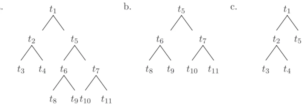
a. t1 t2 t5 t3 t4 t6 t7 t8 t9t10 t11 b. t5 t6 t7 t8 t9 t10 t11 c. t1 t2 t5 t3 t4
Figure 2.1: (a) The treeT, (b) a branch ofT Tt5, (c) the pruned subtreeT
′ =T−T
t5.
2.1.1 Minimal cost-complexity pruning
Minimal cost-complexity pruning was introduced in the CART system (Breiman et al., 1984) for inducing decision trees. This is why it is also called CART pruning. Mini-mal cost-complexity pruning is a kind of post-pruning method. Post-pruning prunes off those branches that are not predictive after a decision tree has been fully ex-panded. When minimal cost-complexity pruning prunes a fully-grown tree back, it considers not only the misclassification cost but also the complexity cost of the tree. In other words, minimal cost-complexity pruning seeks decision trees that achieve a compromise between misclassification cost and tree complexity. Most other pruning methods such as reduced-error pruning (Quinlan, 1987) only consider misclassification cost. Thus, the trees generated by minimal cost-complexity are normally smaller than those generated by other pruning methods.
The principle of minimal cost-complexity pruning
To understand how minimal cost-complexity pruning works, the concept of pruned subtrees needs to be described first. According to Breiman et al. (1984), a pruned subtree T′ is obtained by pruning off a branch T
t from a tree T (i.e. T′=T −Tt),
which replaces Tt with only its root node. The pruned subtree is denoted by T′ ≺T.
Figure 2.1 demonstrates how to obtain the pruned subtree T′ from T. Figure 2.1(a)
shows the original treeT. Figure 2.1(b) shows a branch ofT Tt5. Figure 2.1(c) shows
the pruned subtreeT′=T−T
t5, which is obtained by pruning offTt5 fromT.
The underlying idea of minimal cost-complexity pruning is the following definition: DEFINITION (Breiman et al., 1984)For any subtreeT 4Tmax, define its complexity
complexity parameter and define the cost-complexity measure Ra(T) as
Rα(T) =R(T) +α|Te|.
In this definition,Tmax stands for a fully-grown tree. T stands for a pruned subtree.
R(T) represents the misclassification cost of T on the training data. Thus, the cost-complexity measure is formed by the combination of the misclassification cost and a cost penalty for the tree complexity.
The next step of minimal cost-complexity pruning is to find the pruned sub-tree T(α)4 Tmax which minimisesRα(T) for each value ofα (Breiman et al., 1984), i.e.,
Rα(T(α)) = min T4Tmax
Rα(T).
However, Tmax is sometimes not a good starting point to seek α values because a
pruned subtree Tb may have the same misclassification cost on the training data as
the Tmax while the complexity of Tb is smaller (Breiman et al., 1984). Under these
circumstances, it is obvious that Tb is a better starting point than Tmax. Suppose
that T1 is the smallest pruned subtree of Tmax whose classification cost is equal to
the one ofTmax. ThenT1is treated as the starting point of the whole pruning process.
For any nonterminal node t of T1, denote by Tt the branch of T1 whose root
node is t. If Tt is replaced by t, the pruned subtree T-Tt normally has Ee more
misclassified training instances than T1. Denote the total number of the training
instances asN and define a function (Breiman et al., 1984):
g(t) = Ee
N(|Tet| −1)
.
The heart of minimal cost-complexity pruning is to calculate each value ofα, relative to each pruned subtree. The key to calculating each value ofα is to understand that it works by weakest-link cutting (Breiman et al., 1984). Weakest-link cutting works here by considering theweakest link t1 as the node such that
g(t1) = min
Tk Tek αk Tk Tek αk T1 61 0.0 T9 10 0.0096 T2 58 0.0005 T10 8 0.0120 T3 50 0.0012 T11 7 0.0144 T4 45 0.0013 T12 5 0.0160 T5 17 0.0016 T13 4 0.0240 T6 14 0.0021 T14 3 0.0336 T7 13 0.0048 T15 2 0.0496 T8 11 0.0072 T16 1 0.1744
Table 2.1: The sequence of pruned subtrees from T1, accompanied by their
corre-spondingα values on the balance-scale dataset.
Then the value of g(t1) is the value of complexity parameter for the pruned subtree
T1-Tt1 and denoted as α2. The pruned subtreeT1-Tt1 is denotedT2.
Now, by using T2 as a starting tree instead of T1, the next step is to find t2
in T2 by weakest link cutting and calculate the corresponding value of α α3. This
process is similar to the previous calculation oft1. After this step, the second pruned
subtreeT3,T2 -Tt2 is obtained. This process is repeated recursively until the pruned
subtree to be pruned only has the root node. Thus, a decreasing sequence of pruned subtrees T1 ≻ T2 ≻ T3. . . Tn and an increasing sequence of their corresponding α
valuesα1 < α2< α3. . . αn are formed. Tn stands for the pruned subtree fromT1 that
only has the root node. αn stands for the α value corresponding to Tn. Because T1
is an unpruned tree, its corresponding value ofα α1 is 0. The reason why the values
ofαare strictly in increasing order is shown in the CART book (Breiman et al., 1984). Table 2.1 shows example values generated in the process of minimal cost-complexity pruning in the CART decision tree on the balance-scale dataset from the UCI repository (Blake et al., 1998). The sequence of pruned subtrees, their size in terminal nodes and corresponding α values are listed in the table. As discussed by Breiman et al., the pruning algorithm tends to prune off large subbranches first. For example, it prunes 28 nodes from T4 to T5 in Table 2.1. When the trees are getting
smaller, it only prunes off small subbranches, which is also illustrated in Table 2.1, e.g. from T11 to T12, to T13, and so on. The problem of minimal cost-complexity
pruning is now reduced to selecting which pruned subtree is optimum from the sequence. This can be done by cross-validation.
Cross-validation in minimal cost-complexity pruning
Cross-validation is the preferred method for error estimation when the data sample is not large enough to form one separated large hold-out set. It can significantly reduce sample variance for small data. In V-fold cross-validation, the original data, denoted by L, is randomly divided intoV subsets, Lv, v = 1, 2, . . ., V. In our experiments,
in order to make all subsets representative in both training and test sets L, the original data is stratified first in this thesis. Each subset Lv is held out in turn and
the remaining V-1 subsets are used to grow a decision tree and fix the values of the complexity parameter α for a sequence of pruned subtrees. The holdout subset (e.g. test set) is then used to estimate misclassification cost. Thus, the learning procedure is executedV times on different training sets and test sets.
Each instance in the original data L is used for testing only once in the cross-validation. Thus, if the number of instances of class j misclassified in the vth fold is denoted by Nvj, the total number of misclassified instances for class j on all test
sets (i.e. in all folds) is the sum of Nvj, v = 1, 2, . . ., V, denoted by Nj. The idea
now is to measure the number of misclassified instances of all classes on L in the cross-validation. Assuming T1 is built on all data L and T(α) is a pruned subtree
from T1, the cross-validated misclassification cost of T(α) can be written as:
Rcv(T(α)) = 1/NX
j
Rcv(j),
whereN is the total number of test instances. Suppose a sequence of pruned subtrees
Tk is grown from the full dataset L and their corresponding complexity parameter
values αk, k = 1,2, . . . K, are then obtained. The idea of minimal cost-complexity
pruning is to find the value of the complexity parameter, αf inal, corresponding to
the pruned subtree Tf inal from the sequenceTk which has the minimal expected
mis-classification cost according to the cross-validation. As mentioned before, αk is an
increasing sequence ofα values. Define (Breiman et al., 1984)
αk′ =√αkαk+1
so thatα′
kis the geometric midpoint of the intervalTα=Tk. For eachα′kwe then find
the corresponding tree from each of the training sets in the cross-validation (i.e. the tree that would have been generated by pruning based on that valueα′
k Tek αk Rcv(Tk) seed=1 Rcv(Tk) seed=2 1 61 0.0 0.2291 0.2116 2* 58 0.0005 0.2292 0.2100 3 50 0.0012 0.2260 0.2148 4 45 0.0128 0.2178 0.2164 5 17 0.016 0.21629 0.2164 6 14 0.0021 0.2195 0.2131 7* 13 0.0048 0.21628 0.2163 8 11 0.0072 0.2322 0.2340 9 10 0.0096 0.2548 0.2483 10 8 0.012 0.2692 0.2708 11 7 0.0144 0.2836 0.2804 12 5 0.016 0.2868 0.3013 13 4 0.024 0.3317 0.3413 14 3 0.0336 0.3429 0.3541 15 2 0.0496 0.4134 0.4134 16 1 0.1744 0.5433 0.5417 Table 2.2: Rcv(T
k) for different seeds without 1SE on thebalance-scale dataset.
error is used to computeRcv(T(α′
k)). The value ofα′kfor whichRcv(T(α′k)) is minimal
is used asαf inal. The tree Tf inal is the one that corresponds to the upper bound of
the interval from the sequence of pruned subtreesTkthat was used to computeαf inal.
The 1SE rule in minimal cost-complexity pruning
Because the 1SE rule is also used in pre-pruning and post-pruning for best-first decision trees later in this thesis, it is discussed in a bit more detail here. The reason why the 1SE rule used in minimal cost-complexity pruning is that, for some datasets the pruned subtree that minimisesRcv(T
k) is unstable. Small changes in parameter values or even
the seed used for randomly selecting the data for each fold of the cross-validation may result in very differentTf inal(Breiman et al., 1984). For example, Table 2.2 shows the
effects between different seeds, 1 and 2, in terms of the estimated misclassification cost of the pruned subtrees on the balance-scale dataset from the UCI repository (Blake et al., 1998).
From the table, for seed 1, T7 with 13 terminal nodes is selected as the final pruned
subtree. For seed 2,T2 with 58 terminal nodes is selected. The selected subtrees are
significantly different. The 1SE rule can be used to avoid this problem and choose similar pruned subtrees. It has two objectives in minimal cost-complexity pruning (Breiman et al., 1984). One is to reduce the instability of choosingTf inal. The other is
k Tek αk Rcv(Tk) seed=1 Rcv(Tk) seed=2 1 61 0.0 0.2291±0.0168 0.2116±0.0163 2 58 0.0005 0.2292±0.0168 0.2100±0.0163 3 50 0.0012 0.2260±0.0167 0.2148±0.0164 4 45 0.0128 0.2178±0.0165 0.2164±0.0165 5 17 0.016 0.21629±0.0165 0.2164±0.0165 6 14 0.0021 0.2195±0.0166 0.2131±0.0164 7* 13 0.0048 0.21628±0.0165 0.2163±0.0165 8* 11 0.0072 0.2322±0.0169 0.2340±0.0169 9 10 0.0096 0.2548±0.0174 0.2483±0.0173 10 8 0.012 0.2692±0.0177 0.2708±0.0178 11 7 0.0144 0.2836±0.0180 0.2804±0.0180 12 5 0.016 0.2868±0.0181 0.3013±0.0184 13 4 0.024 0.3317±0.0188 0.3413±0.0190 14 3 0.0336 0.3429±0.0190 0.3541±0.0191 15 2 0.0496 0.4134±0.0197 0.4134±0.0197 16 1 0.1744 0.5433±0.0199 0.5417±0.0199 Table 2.3: Rcv(T
k) for different seeds with 1SE on thebalance-scale dataset.
to find the simplest pruned subtree whose performance is comparable to the minimal value of Rcv(T
k) Rcv(Tk0) in terms of accuracy. Denote by N the total number of
instances in the original data. The standard error estimate for Rcv(Tk) is defined as
(Breiman et al., 1984):
SE(Rcv(Tk)) = [Rcv(Tk)(1−Rcv(Tk))/N]1/2.
Then the selection of Tf inal, according to the 1SE rule (Breiman et al., 1984), is the
smallest pruned subtree Tk1 satisfying Rcv(Tk1)≤R
cv(T
k0) +SE(R
cv(T k0)).
Continuing the example shown in Table 2.2, Table 2.3 presents Rcv(T
k) with 1SE.
According to the 1SE rule, the selection of Tf inal is now different from the previous
selection. T8 with 11 terminal nodes and T7 with 13 terminal nodes are selected
respectively. The Tf inal trees are now stable.
Overfitting in minimal cost-complexity pruning
Oates and Jensen (1997) investigated the effects of training set size on tree complexity for four pruning methods based on the trees generated by C4.5 (Quinlan, 1993) on 19 UCI datasets. These four pruning methods are error-based pruning (Quinlan, 1993),
reduced-error pruning (Quinlan, 1987), minimum description length pruning (Quinlan & Rivest, 1989) and minimal cost-complexity pruning. The experimental results indicate that the increase of training set size often results in the increase in tree size, even when that additional complexity does not improve the classification accuracy significantly. That is to say, the additional complexity is redundant and it should be removed. Oates and Jensen found that minimal cost-complexity pruning appropri-ately limited tree growth much more frequently than the other three pruning methods. A special example was given by Oates and Jensen considering four pruning al-gorithms on the australian dataset. Minimal cost-complexity pruning is compared both with and without the 1SE rule. According to the paper, accuracy peaks with a small number of training instances. After that, it remains almost constant. However, tree size continues to increase nearly linearly in error-based pruning, reduced-error pruning and minimum description length pruning. Said differently, the trees pruned by these pruning methods are overfitted. Minimal cost-complexity pruning does not suffer from this problem on the dataset. If the 1SE rule is applied, tree size stays almost constant after a small number of the training instances is used. If the 1SE rule is not applied, tree size stays within a stable range after a small number of training instances is input.
2.1.2 Other pruning methods related to cross-validation
Cross-validation can also be used in critical value pruning (Mingers, 1987), reduced-error pruning (Quinlan, 1987) and the wrapper approach (Kohavi, 1995a). Critical value pruning uses cross-validation to decide the threshold of the pruning, where the threshold is the key to determining tree size. Frank (2000) apply the combination of statistical significance tests and cross-validation in reduced-error pruning to seek an optimal significance level. The wrapper approach searches a subset of features and tune their parameters to obtain the model with the best performance based on cross-validation.
Cross-validation in critical value pruning
Critical value pruning (Mingers, 1987) is a bottom-up technique like minimal cost-complexity pruning. However, it does not use a pruning set. When growing a tree, the pruning procedure considers the splitting information of each node. Recall
that at each node of a standard decision tree, splitting happens on the attribute which can maximally reduce impurity, or in other words, maximise the value of the splitting criterion, for example, Gini gain in the CART system. Critical value pruning prunes off branches based on this value. It first sets up a fixed threshold for the splitting criterion. Once the value of the splitting criterion corresponding to a node is less than the threshold, the node is made into a terminal node. One additional constraint is that, if the branch contains one or more nodes whose value is greater than the threshold, it will not be pruned.
The problem is now how to determine the threshold. Clearly, if the threshold is too large, the pruning is aggressive and it results in too small trees. On the contrary, if the threshold is too small, the pruning results in too large trees and can not prevent overfittng effectively. This is why cross-validation is suitable in this situation. The goal of cross-validation here is to find the best value of the threshold which leads to trees with reasonable size and good performance.
Cross-validation in reduced-error pruning
Standard reduced-error pruning is known to be one of the fastest pruning algorithms, producing trees that are both accurate and small (Esposito et al., 1997). The idea of reduced-error pruning is that it divides the original data into a training set and a pruning set (i.e. test set). The tree is fully grown on the training set and then the pruning set is used to estimate the error rate of branches. It prunes off unreliable branches in a bottom-up fashion. If replacing a branch with the root of the branch reduces the error on the pruning set, the branch is pruned. However, this pruning method suffers from overfitting the pruning data (Oates & Jensen, 1997), which results in an overly complex tree because the pruning data is used for multiple pruning decision. This problem is similar to the overfitting problem on the training data.
Frank (2000) investigated standard reduced-error pruning accompanied with statistical significance tests based on cross-validation to avoid the problem of overfit-ting the pruning set. In his experiments, the significant level is set as a parameter to optimise the performance of the pruned trees. The value of optimised significance level is obtained based on cross-validation. Experiments on 27 datasets from the UCI
repository (Blake et al., 1998) shows that the tree size in 25 datasets is significantly smaller than before and the accuracy only significantly decreases in 5 datasets.
Cross-validation in the wrapper approach
For an induction algorithm, different parameter settings result in different perfor-mances in most cases. In fact, every possible parameter setting of an algorithm can be treated as a different model. The wrapper approach (Kohavi, 1995a) is based on this observation. Given an algorithm, the goal of the wrapper approach is to search a subset of features and tune their parameters to obtain the model with the best perfor-mance. Cross-validation is used as the evaluation function in the tuning of parameters. Kohavi and John (1995) compared C4.5 (Quinlan, 1993) with default parame-ter setting to C4.5 with automatic parameparame-ter tuning on 33 datasets. In the automatic parameter tuning, four parameters are adjusted, namely, the minimal number instances at terminal nodes, confidence level, splitting criterion and the number of branches for a node. They pointed that if the confidence level is set to 0.9, C4.5 with automatic parameter tuning is significantly better than C4.5 with default parameter setting on nine datasets, and the latter one is significantly better on only one dataset. In the case where C4.5 with default parameter setting is better, the entire dataset is very small with only 57 instances. If the confidence level is set to 0.95, C4.5 with automatic parameter tuning outperforms C4.5 with default parameter setting on six datasets and is never outperformed by the latter one.
2.2
Pruning in standard decision trees
Pruning algorithms are designed to avoid overfitting and sample variance. They stop splitting early or discard those branches which have no improvement in performance (e.g. the accuracy in most cases). Generally speaking, there are two sorts of pruning, pre-pruning and post-pruning. Pre-pruning stops splitting when information becomes unreliable (e.g. no statistical significance in the most popular cases). Post-pruning takes a fully-grown tree and pruning off those branches that are not predictive. This section briefly describes the principles of pre-pruning and post-pruning algorithms for standard decision trees. Then, comparisons of pre-pruning and post-pruning are discussed.
2.2.1 Pre-pruning and post-pruning
As mentioned before, pre-pruning stops splitting when the splitting cannot improve predictive performance. In decision trees, pre-pruning is actually a problem of attribute selection (Frank, 2000). In other words, it selects those attributes which are predictive for the class. Pre-pruning only use local attribute selection: given a set of attributes in each node of a decision tree, find those attributes that are relevant to predict the class to split on. If no relevant attribute is found, this split stops and the current node is made into a terminal node. Otherwise, the node is split based on one of the predictive attributes. A predictive attribute means that there is a significant association between this attribute and the class. Thus, the goal of pre-pruning is to find whether a attribute is significantly correlated to the class. Statistical significance tests such as the chi-squared test, are designed for this kind of situation. Statistical significance tests can determine whether an observed association is a reflection of the real representation underlying the data sample or it is generated by random chance. The problem now becomes, given a set of attributes at each node of a decision tree, finding whether there is any statistical significance; if statistical significance exists, how to select an attribute to split the training set into subsets. Otherwise, stop splitting the training set and make the node into a terminal node. The chi-squared test is traditionally used as a statistical significant test. For example, Quinlan’s ID3 decision tree (1986) uses it to decide when to stop splitting the training set. The same technique is also used by the decision tree inducer CHAID (Kass, 1980). The idea behind the chi-squared test is that information in a small data sample may not be reliable. The question is now simplified to find the attribute with the optimum value of the splitting criterion to split on among all attributes for which the chi-squared test shows a significant association with the class. Potential problems with pre-pruning are discussed below.
Post-pruning takes a fully-grown tree and prunes off those branches that are not predictive such as the pruning methods discussed in the previous section. Most post-pruning procedures prune branches according to classification error. In other words, post-pruning prunes off branches which do not improve accuracy. Although, in theory, statistical significance tests can be used to determine whether a branch should be split in both pre-pruning and post-pruning, most standard post-pruning
a b class 0 0 0 0 1 1 1 0 1 1 1 0
Table 2.4: A parity problem.
algorithms do not involve significance tests. Moreover, most post-pruning algorithms prune trees use a bottom-up fashion such as reduced-error pruning.
2.2.2 Comparisons of pre-pruning and post-pruning
Historically, pre-pruning techniques were investigated before post-pruning techniques. The pre-pruning methods of the earliest decision tree algorithms were introduced to deal with noisy data. Since then, pre-pruning had largely been discarded when two influential books by Breiman et al. (1984) and Quinlan (1993) were brought forth. Clearly, pre-pruning is faster than post-pruning because it stops splitting earlier. However, pre-pruning is assumed to be inferior to post-pruning because it might encounter the problem of interaction effects. The problem is that, in univariate decision trees each test is only based on a single attribute, so pre-pruning might overlook the effect of several interacting attributes and stop growing trees too early. Post-pruning does not suffer from this problem because the interaction effects are visible in fully-grown trees.
The parity problem is a typical example of interaction effects at work. A dataset shown in Table 2.4 is an example of this problem. The dataset has two binary attributes,a and b. Each attribute has two values, 0 and 1. The class is also binary and it has two labels 0 and 1. Given any single attribute, both classes are equally likely. Clearly, no individual attribute exhibits any significant association to the class, so no further split will be performed. Post-pruning is not influenced because the pruning starts with a fully-expanded tree and it can retain fully expanded branches. The fully-grown tree for this data is shown in Figure 2.2.
However, Frank (2000) found that, on the real-world datasets, parity problems have very little influence on performance differences between pre-pruning and post-pruning. Frank attempted a fair comparison of pre-pruning and post-pruning using the same
a 0 1 b 0 1 b 0 1 0 1 1 0
Figure 2.2: The tree for the parity problem.
statistical significance criteria. He executed his investigation on 27 datasets from the UCI repository (Blake et al., 1998). According to his research, the performance differences can be eliminated by adjusting the significance level for the two pruning individually and the performance differences only happen if a significance level is fixed. Moreover, he showed that, on the real-world datasets he investigated, parity problems have very little influence on performance differences between pre-pruning and post-pruning.
The question is now which pruning procedure should be chosen. The sugges-tion is that, for very large datasets, pre-pruning methods may be preferable because they are much faster. For small datasets or large datasets where time is not a factor, post-pruning methods may be preferable because they could guarantee that the parity problems cannot cause problems.
2.3
Best-first decision trees in boosting
Best-first decision trees have so far been only evaluated in the context of boosting algorithms (Friedman et al., 2000) and no pruning methods were applied to them. Boosting is a supervised machine learning technique that combines the performance of many ”weak” classifiers (i.e. those that have an accuracy greater than chance) to produce a powerful ”committee”. The basic idea underlying boosting is that, given a dataset, each training instance is first assigned an equal weight. Then, the dataset is used to form ”weak” models repeatedly. New models are influenced by the performance of previously built ones by re-weighting the training instances. Finally, all models are averaged or voted to build the final model and predict class values. The final model is actually a combination of all the models produced in the iterations of the boosting algorithm. There are several different boosting algorithms, depending
on the exact way of weighting instances and models.
Friedman et al. (2000) investigated four boosting algorithms, LogitBoost, Real AdaBoost, Gentle AdaBoost and Discrete AdaBoost using decision trees as base learners. Generally, when decision trees are applied to boosting, the growing and pruning of trees are normally the same as trees are built in isolation. However, pruning is sometimes not necessary as the trees can be restricted to a fixed size instead in boosting. According to Friedman et al. (2000), although building large trees decreases the error rate of each individual model, it increases the error rate of the final model in all four boosting algorithms. Friedman et al. (2000) also found that after enough iterations of boosting were performed, the stump-based model (a tree that only has two terminal nodes) produced superior accuracy.
The task is thus to find a tree which can improve accuracy while restricting the depth of the tree to be not much larger than the actual tree. The depth of the tree is called a ”meta-parameter” (Friedman et al., 2000). It is clear that the ”meta-parameter” is unknown in advance for different datasets. To achieve the goal, one possibility is to first grow a fully expanded tree and then use standard pruning methods to prune it back. However, it is computationally wasteful because the iterations of boosting normally are executed many times.
Another possibility is to stop growing the tree early at the specified size, which can reduce computation time significantly. Under these circumstances, it is necessary to define the order of splitting nodes so that maximum use is made of the limited size. This is how the best-first tree works. The best-first tree first splits the node which maximally reduces the impurity among all nodes available to split. It continues this step until a fixed number M of terminal nodes is reached. Because M is the parameter for all trees in the boosting algorithm, it is also the parameter for the boosting algorithm itself. Thus, its value can be obtained by parameter selection based on cross-validation. This combination of truncated best-first decision trees with boosting shows excellent performance in the experiments by Friedman et al. (2000). They compared their experimental results to the corresponding results for boosting reported by Dietterich (1998) and pointed out that, the error rates with small truncation values are quite favourable to other committee approaches
with much larger trees at each iteration. Even if the accuracy is the same, the computation time is dramatically smaller. In this thesis, the same best-first decision tree growing strategy is evaluated in the context of pruning stand-alone trees.
2.4
Summary
This chapter concerns the background of this thesis. We discussed some pruning methods based on cross-validation. Minimal cost-complexity pruning was discussed in detail because it would be compared to pre-pruning and post-pruning with best-first decision trees in this thesis. Minimal cost-complexity pruning is a pruning procedure which considers not only misclassification cost but also complexity cost for decision trees. In the description, the 1SE rule was also presented, which can guarantee the stability of the final selected pruned subtree. Then, cross-validation in critical value pruning, reduced-error pruning and the wrapper approach was briefly discussed. Then, the principles of pre-pruning and post-pruning for standard decision trees were discussed. Pre-pruning stops splitting a node of a decision tree if there is no statistical significance. Post-pruning prunes off branches of a fully-grown tree back which cannot improve performance. The advantages and disadvantages of pre-pruning and post-pruning in standard decision trees were also discussed. The suggestion is that, for very large datasets, pre-pruning may be preferable because it is faster. For small datasets or large datasets where time is not a factor, post-pruning may be the better choice because it guarantees that parity problems cannot cause problems. Lastly, the work related to best-first decision trees was discussed. In this work, best-first decision trees are applied to boosting. This work shows that, if the number of iterations is large enough, boosting with small decision trees can produce good results. Thus, it is a good idea to decide the order of nodes to split. Best-first decision trees fulfil this requirement. Error rates of ensembles with small trees are quite favourable to other committee approaches with much larger trees built in each iteration. And even if the accuracy is the same, the computation time can be dramatically smaller.
Chapter 3
Best-first decision tree learning
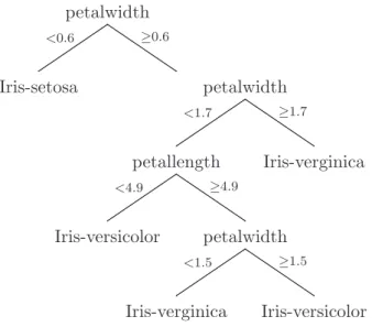
Best-first decision tree learning is a kind of decision tree learning, and thus it has almost all properties of standard decision learning. Decision tree learning is one of the most popular learning approaches in classification because it is fast and produces models with good performance. Generally, decision tree algorithms are especially good for classification learning if the training instances have errors (i.e. noisy data) and attributes have missing values. A decision tree is an arrangement of tests on attributes in internal nodes and each test leads to the split of a node. Each terminal node is then assigned a classification. In practice, in most decision tree algorithms, each internal node tests only one attribute such as in ID3 (Quinlan, 1986) although a test can be based on a set of attributes with a corresponding loss of interpretability. The best-first decision tree algorithm presented in this thesis only uses tests on one attribute. Thus, from now on, all tests we talk about are based on a single attribute. A simple example tree is shown in Figure 3.1, which has been obtained by applying the best-first decision tree algorithm on the iris dataset. The minimal number of instances at the terminal nodes was set to two. In general, decision trees represent a disjunction of conjunctions of constraints on the attribute-values of instances. Each path from the root to a terminal node corresponds to a conjunction of at-tribute tests, and the tree itself to a disjunction of these conjunctions (Mitchell, 1997). When building models, decision tree algorithms separate instances down the tree from the root node to the terminal nodes. Each terminal node provides a classification. Each internal node in the tree specifies a test of an attribute of the instances, and each branch is based on a subset of the values of the instances for this attribute. When classifying an instance, the decision tree algorithms start at the root node, test the attribute specified by this node, and then move down to the tree branch corresponding to the value of the attribute. This process is then repeated until a terminal node is reached. The classification of the terminal node is
petalwidth <0.6 ≥0.6 Iris-setosa petalwidth <1.7 ≥1.7 petallength <4.9 ≥4.9 Iris-verginica Iris-versicolor petalwidth <1.5 ≥1.5 Iris-verginica Iris-versicolor Figure 3.1: The best-first decision tree on the iris dataset. the predicted value for the instance.
Trees generated by best-first decision tree learning have all properties described above. The only difference is that, standard decision tree learning expands nodes in depth-first order, while best-first decision tree learning expands the ”best” node first. Standard decision tree learning and best-first decision tree learning generate the same fully-expanded tree for a given data. However, if the number of expansions is specified in advance, the generated trees are different in most cases. For example, Figure 3.2 shows a hypothetical standard decision tree and a hypothetical best-first decision tree with three expansions on the same data. The first tree in the figure is the fully-expanded tree generated by best-first decision tree learning and the second tree is the fully-expanded tree generated by standard decision tree learning. In this example, considering the fully-expanded best-first deci-sion tree the benefit of expanding nodeN2 is greater than the benefit of expandingN3.
The rest of this chapter is organised as follows. Section 3.1 describes two splitting criteria to measure impurity in best-first decision trees that are investigated in this thesis: information and Gini index. The methods of calculating reduction of impurity, namely, information gain and Gini gain, are also discussed and examples are given on the weather dataset. Section 3.2 discusses splitting rules used in best-decision decision trees presented in this thesis. The goal of the splitting rules is to find the ”best” binary split for both numeric attributes and nominal attributes. The ”best”
a. N
1
N3 N2
Leaf N4 Leaf Leaf
Leaf Leaf
b. N
1
N2 N4
Leaf N3 Leaf Leaf
Leaf Leaf
c. N
1
N3 N2
Leaf Leaf Leaf Leaf
d. N
1
N2 Leaf
Leaf N3
Leaf Leaf
Figure 3.2: (a) The fully-expanded best-first decision tree; (b) the fully-expanded standard decision tree; (c) the best-first decision tree with three expansions from (a); (d) the standard decision tree with three expansions from (b).
split is the split with the maximal reduction of impurity. Section 3.3 presents the algorithm of best-first decision tree learning. The method of dealing with missing values is also discussed in this section. Section 3.4 discusses two pruning methods for best-first decision trees. We explain how the 1SE rule can be used in the pruning process. Section 3.5 discusses complexity of best-first decision tree induction. Section 3.6 summarises this chapter.
3.1
Splitting criteria
In order to find the ”best” node to split at each step of best-first decision trees, splitting criteria must be addressed. There are many criteria for decision trees and two of them are most widely used, the information and the Gini index. For example, the information is used in ID3 (Quinlan, 1986) and C4.5 (Quinlan, 1993), and the Gini index is used in the CART system (Breiman et al., 1984). Best-first decision trees can also use these two criteria.
outlook temperature humidity windy play sunny 85 85 false no sunny 80 90 true no overcast 83 86 false yes rainy 70 96 false yes rainy 68 80 false yes rainy 65 70 true no overcast 64 65 true yes sunny 72 95 false no sunny 69 70 false yes rainy 75 80 false yes sunny 75 70 true yes overcast 72 90 true yes rainy 81 75 false yes rainy 71 91 true no Table 3.1: The instances of theweather dataset.
based on the distribution of classes. Recall that the main objective of decision tree learning is to obtain accurate and small models. Thus, when splitting a node, we should find pure successor nodes as early as possible. In other words, the goal of splitting is to find the maximal decrease of impurity at each node. The decrease of impurity is calculated by subtracting the impurity values of successor nodes from the impurity of the node. When the subtraction is performed, the impurity values of the successor nodes are weighted by the size of each node: the number instances reaching each node. If the splitting criterion is the information, the decrease in impurity is measured by the information gain. Similarly, if the splitting criterion is the Gini index, the decrease in impurity is measured by the Gini gain.
When describing the splitting criteria, we use the weather dataset as an exam-ple to explain the calculation of the information and the Gini index in best-first decision trees. The reduction of impurity, namely, the Gini gain or the information gain, is also discussed. The weather dataset has fourteen instances. Every instances has four attributes, outlook, temperature, humidity and windy, and the class play. Attribute outlook is nominal and it has three values, sunny, overcast and rainy. Attributes temperature and humidity are numeric. Attribute windy is binary and it has two values,true andfalse. The classplay is binary. The fourteen instances of the
3.1.1 Information
Information is the most widely used splitting criterion to measure impurity and it is expressed in units called bits. The bits in information calculation are fractions and they are normally less than 1. The information is based on the distribution of classes as mentioned before. The information value is called entropy. For a general dataset which hasnclasses, the entropy is defined as (Quinlan, 1986):
entropy(p1, p2, . . . , pn) =−p1logp1−p2logp2. . .−pnlogpn,
where pk, k= 1, 2, . . .,n, is the probability of each class and the sum of thepk is 1.
Normally, the base of the logarithms is two and this is the reason why the result can be viewed ”bits”. The reason for the minus signs is that logarithms of the fractions
pk are negative. Thus, the entropy is positive. Note that ifpkis 0 logpk is set to 0 in
the calculation. Then, the information value can be estimated by the formula:
inf o([P1, P2, . . . , Pn]) =entropy(p1, p2, . . . , pn),
where Pk, k = 1, 2, . . ., n, is the number of instances for each class. The estimated
value of pk is the value of Pk divided by the sum of allPk.
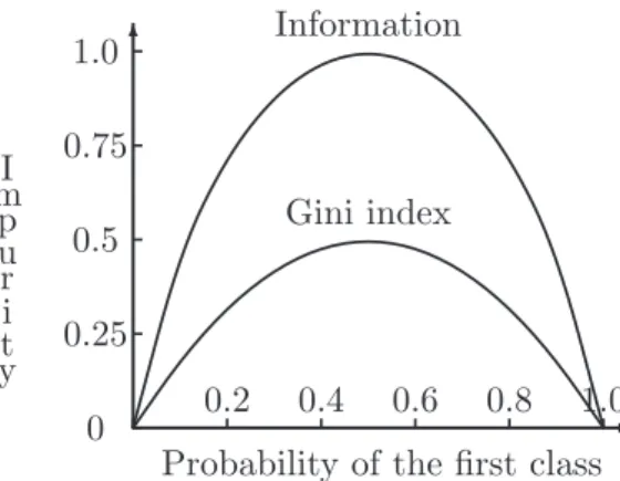
According to the formula, the purer a node is, the smaller the information value will be. For a absolutely pure node, namely, for which one class probability is 1 and the other class probabilities are 0, the information value is 0. For a two-class problem, the entropy is −p1logp1−p2logp2, where the sum of p1 and p2 is 1. The
relationship between the information value and the class probability of the first class in the two-class problem is shown in Figure 3.4.
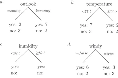
Recall that this thesis investigates binary decision trees. Figure 3.3 lists four possible splits as examples to calculate information values, one for each attribute in the weather dataset. Let us evaluate the first split in Figure 3.3 now. The class distributions (i.e. yes/no) for the two successor nodes are 2/3 and 7/2 respectively. The information values for the root node and the two successors nodes are thus
inf o([9,5]) =entropy(149,145 ) =−149 log149 −145 log145 = 0.940bits inf o([2,3]) =entropy(25,35) =−52log25 −35log35 = 0.971bits