American Institute of Aeronautics and Astronautics 1
Fluorescence visualization of hypersonic flow past triangular and
rectangular boundary-layer trips
P.M. Danehy*, A.P. Garcia†, S. Borg‡, A.A. Dyakonov§, S.A. Berry**, J.A. (Wilkes) Inman††, D.W. Alderfer‡‡ NASA Langley Research Center, Hampton VA, 23681-2199
Planar laser-induced fluorescence (PLIF) flow visualization has been used to investigate the hypersonic flow of air over surface protrusions that are sized to force laminar-to-turbulent boundary layer transition. These trips were selected to simulate protruding Space Shuttle Orbiter heat shield gap-filler material. Experiments were performed in the NASA Langley Research Center 31-Inch Mach 10 Air Wind Tunnel, which is an electrically-heated, blowdown facility. Two-mm high by 8-mm wide triangular and rectangular trips were attached to a flat plate and were oriented at an angle of 45 degrees with respect to the oncoming flow. Upstream of these trips, nitric oxide (NO) was seeded into the boundary layer. PLIF visualization of this NO allowed observation of both laminar and turbulent boundary layer flow downstream of the trips for varying flow conditions as the flat plate angle of attack was varied. By varying the angle of attack, the Mach number above the boundary layer was varied between 4.2 and 9.8, according to analytical oblique-shock calculations. Computational Fluid Dynamics (CFD) simulations of the flowfield with a laminar boundary layer were also performed to better understand the flow environment. The PLIF images of the tripped boundary layer flow were compared to a case with no trip for which the flow remained laminar over the entire angle-of-attack range studied. Qualitative agreement is found between the present observed transition measurements and a previous experimental roughness-induced transition database determined by other means, which is used by the shuttle return-to-flight program.
I. Introduction
mall structures protruding from a hypersonic vehicle’s surface can force the boundary layer to transition to turbulent flow prematurely. While this can be a desirable effect – for example, on a scramjet inlet where turbulent flow might be desired to enhance fuel-air mixing – it is detrimental in applications where surface heating is a concern. Transitional and turbulent flows generally cause increased heating on entry vehicles. In the first Space Shuttle Return-to-Flight (RTF) mission, STS-114, a piece of gap filler material was observed, while in orbit, to be protruding from the shuttle orbiter’s heat shield. Such a large piece of gap filler might force the boundary layer flow on the orbiter to transition to turbulent flow much earlier in the flight trajectory than in prior flights.1 To avoid this, a space walk was performed to remove the material. To inform such decisions, NASA has developed the Boundary Layer Transition (BLT) tool to predict the time within the entry trajectory required for a boundary layer to transition into a turbulent flow as a function of type (protuberance or cavity), location, and size (but not shape) of the damaged region of a space vehicle.2 This tool is part of a suite of tools3 used to evaluate any damage to the thermal protection system of the orbiter vehicle and whether necessary steps should be taken to ensure the safe landing of the vehicle upon reentry.
* Research Scientist, Advanced Sensing and Optical Measurement Branch, MS 493, AIAA Associate Fellow. † PhD Student, Department of Physics, College of William and Mary, Williamsburg, Virginia, and Graduate Student Researcher Program (GSRP) Student, Advanced Sensing and Optical Measurement Branch, MS 493.
‡ Research Scientist, Advanced Sensing and Optical Measurement Branch, MS 493 § Research Scientist, MS 489 National Institute of Aerospace, Hampton VA. ** Research Scientist, Aerothermodynamics Branch, MS 408A
†† PhD Student, Department of Physics, College of William and Mary, Williamsburg, Virginia, and NASA Graduate Coop Student, Advanced Sensing and Optical Measurement Branch, MS 493, AIAA Student Member.
‡‡ Research Scientist, Advanced Sensing and Optical Measurement Branch, MS 493
S
American Institute of Aeronautics and Astronautics 2
In addition to NASA’s RTF work described above, a detailed database of heating phenomena downstream of various passive and active trip geometries was developed for the X-43A flight experiment at NASA Langley Research Center.4 In the X-43A work, schlieren flow visualization provided useful information about shock positions, although this information was path-averaged and turbulent flow structures were not identified with the schlieren. Planar laser-induced fluorescence (PLIF) is one of a variety of planar flow visualization techniques that can provide three-dimensionally spatially-resolved off-body visualizations of boundary layers5,6,7 and other hypersonic flow phenomena.8,9,10 PLIF visualizations of the flowfields downstream of boundary layer trips could help to explain how and why transition is occurring. Seeding the flow upstream of the trips with a fluorescing gas allows the flowfield over, around, and downstream of trips to be visualized. This paper is a proof of concept study showing how boundary layers downstream of roughness elements can be visualized using PLIF. We believe that this paper reports the first investigation using PLIF to study transition of flow over trips.
II. Experimental Equipment and Procedures
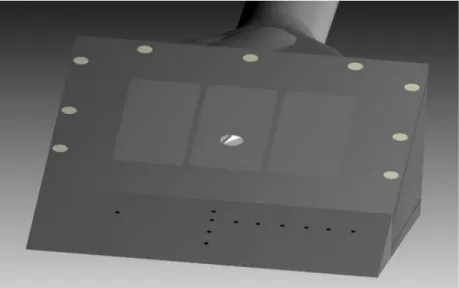
A portable PLIF system was used to study hypersonic flow over two different types of trips in the 31-Inch Mach 10 Wind Tunnel facility at NASA Langley Research Center. Nitric oxide (NO) was used for the fluorescence imaging since it has favorable gasdynamic and spectroscopic properties and because it could be seeded into the flow. NO molecules were excited by an ultra-violet (226 nm) laser sheet, and the resulting fluorescence was captured with an intensified CCD camera. NO was seeded into the flow from four orifices located on the model centerline. The seeded NO became entrained into the air flow and was then imaged. This technique provides flow visualization of flow structures when a boundary layer trip is inserted on a flat plate as depicted in Fig.1.
A. Flat Plate and Trip Designs
The test article was wedge-shaped, with flat plates on top and bottom and a sharp leading edge. The top surface had three large rectangular instrumentation ports on its top surface (see Fig. 1) that could be filled either by instrumentation modules, blanks, or an experiment such as a trip or a cavity. We recently used this hardware to study cavity flows.10 For the present work, triangular and rectangular trips were built and mounted flush with the top, flat surface of the model. The triangular and rectangular shapes of these two trips were modeled after the two that were removed during STS-114.2 To size the trips used in this experiment, the boundary layer thickness needed to be determined for various sting angles of attack. The flat plate viewed in this experiment is the one attached to the top
surface of the model, which had a half angle of 10º. Consequently, the angle of the flat plate relative to the flow is equal to 10º minus the sting angle. The flat plate was 127.0 mm wide and 157.2 mm long. A preliminary estimate of the boundary layer thickness was calculated using Eq. (1):11
⎪⎭ ⎪ ⎬ ⎫ ⎪⎩ ⎪ ⎨ ⎧ − + + = 2.397 0.193Pr1/2( 1) 2 2 / 1 Re 721 . 1 e M e Tw T x x γ δ , (1)
where x = 92.1 mm is the distance from the leading edge of the model to the center of the trip, γ is the ratio of specific heats and is 1.4 for air, Me is the Mach number at the edge of the boundary layer, Tw and Te are the wall temperature and boundary layer edge temperatures respectively, Pr is the Prandtl number, and Rex is Reynolds number based on the edge conditions and distance x. Since the edge conditions were not known during the design
Figure 1. ViDI (Virtual Diagnostics Interface; see section III.B. for details) rendering of the flat plate model tested, showing the triangular trip at the center and the four orifices on the model centerline that were used to seed NO.
American Institute of Aeronautics and Astronautics 3
phase of the experiment, freestream or shock layer values were used instead. As the flat plate angle of attack varied, the gas velocity, Mach number, and density also changed, allowing several different conditions to be visualized with a single model and in a single wind tunnel run. Changing angle of attack significantly changes the boundary layer thickness. For the non-zero flat plate angles of attack, post-shock conditions were calculated using perfect-gas oblique shock relations; these conditions were then used as the freestream and edge conditions for Eq. (1). Table 1 shows the results of this calculation and indicates how the various parameters depend on the sting angle of attack.
Flat Plate
Angle Sting Angle of Attack (freestream, fs, or Mach Number post-shock, ps) Calculated Boundary Layer Thickness (δ) 0º +10º 9.8 (fs) 5.8 mm 10º 0º 6.7 (ps) 2.2 mm 20º -10º 4.2 (ps) 1.5 mm
Table 1. Variation of parameters in the experiment with angle of attack. The boundary layer thickness was calculated analytically using Eq. (1). For purposes of designing the trip height, the freestream Mach number was assumed to be approximately the edge Mach number. The Mach number for the freestream was determined from Ref. 11.
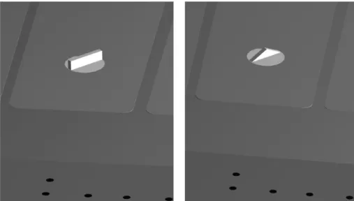
Since the boundary layer thickness ranged from approximately 1.5 mm to nearly 6 mm, the height of both trips was designed to be less than, equal to, and greater than the boundary layer thickness as the sting angle of attack varied. The triangular and rectangular trips both had dimensions of 1 mm thick by 2 mm high by 8 mm wide. They were mounted on the flat plate at an angle of 45º as shown in Figs. 1 and 2. However they were designed in a rotational mounting so they could be oriented at any angle. This experimental geometry was chosen to simulate protruding gap-filler material on the Space Shuttle Orbiter. The gaps between the heat-shield tiles on the Orbiter are generally oriented at a 45º angle with respect to the local flow streamlines on large portions of the windward fuselage. Consequently, protruding gap-filler material is typically oriented at 45º with respect to the boundary layer flow.
Figure 2. Close-up ViDI renderings of the rectangular (left) and triangular (right) trips inserted in the flat plate.
B. Planar laser-induced fluorescence (PLIF) Imaging System
The PLIF system consists primarily of the laser system, beam forming optics and the detection system. The laser system has three main components: a pump laser (Spectra Physics Pro-230-10), a tunable pulsed dye laser (Spectra Physics PDL-2), and a wavelength extender (Spectra Physics WEX). The injection-seeded Nd:YAG laser operates at 10 Hz and pumps the PDL, which contains a mixture of Rhodamine 590 and Rhodamine 610 laser dyes in a methanol solvent. The output of the dye laser and the residual infrared from the Nd:YAG are combined in the WEX, which contains both a doubling and a mixing crystal. The resulting output is tuned to a wavelength of 226.256 nm, chosen to excite the strongly fluorescing spectral lines of NO near the Q1 branch head.
A monitoring gas cell system is used to ensure that the laser is tuned to the correct spectral line of NO. The gas cell contains a low-pressure mixture of 5% NO in N2. A quartz window serves as a beam splitter and sends a small
American Institute of Aeronautics and Astronautics 4 portion of the laser energy through windows on either side of the
gas cell. A photomultiplier tube (PMT) monitors the fluorescence intensity through a third window at right angles to the path of the laser beam.
The components of this laser system are mounted within a two-level, enclosable, portable cart. A photograph of this portable PLIF system is shown in Fig. 3 with the panels removed to show the internal components. When all of the panels are in place, a single monochromatic ultraviolet laser beam exits the cart, creating a relatively safe operating environment. Further details of the system can be found in Reference 12.
For the experiments reported herein, this portable system was installed adjacent to the NASA Langley Research Center’s 31-Inch Mach 10 wind tunnel. Dedicated adjustable scaffolding with attached mirrors and prisms directed the UV laser beam to the top of the wind tunnel test section. Optics then formed the beam into a 100 mm wide by ~1 mm thick laser sheet, which was directed vertically downward through a window in the top of the test section. The section of scaffolding directly above the test section was mounted to a translation stage that could be remotely controlled so that the laser sheet could be swept spanwise through the flowfield during a tunnel run. This was used for alignment of the laser sheet and also for scanning the image plane through the flowfield to visualize three-dimensional flow structures. The resulting fluorescence from NO molecules in the flow was imaged onto a gated, intensified CCD camera. A 3-mm thick Schott glass UG5 filter was placed in front of the camera lens in order to attenuate scattered light at the laser’s frequency. This
was particularly important when the laser sheet impinged on the surface of the model, potentially resulting in direct reflections towards the camera.
Flow visualization images were acquired at 10 Hz with a 1 µs camera gate and a spatial resolution of approximately 5 to 7 pixels/mm, varying from run to run as different camera views and laser sheet orientations were used. The camera was oriented about 10° above the model and about 20° downstream of the laser sheet to allow viewing behind the trip. Thus, the raw images had significant perspective distortion that was later removed with image processing. An image of a “dot card” (a flat piece of paper having a regular pattern of square dots) was acquired with each positioning of the CCD camera, and this dot card image afforded the necessary reference for dewarping the fluorescence images. The temporal and spatial resolutions were more than sufficient to resolve flow structures of interest.
C. Wind Tunnel, Operating Conditions, Mass Flow Control and Data Acquisition Systems
The 31-Inch Mach 10 Air wind tunnel is an electrically-heated blowdown facility located in Building 1251 at NASA Langley Research Center in Hampton, Virginia, USA. Reference 13 details this facility, a summary of which is provided here. As the name implies, the facility has a nominal freestream Mach number of 10 at the a 31-inch square test section. The tunnel uses heated, dried, and filtered air as the test gas. The air flows from the high pressure heater, through the settling chamber, three-dimensional contoured nozzle, test section, second minimum, aftercooler and into vacuum spheres pumped by a steam ejector and conventional vacuum pumps. The test section is “closed,” as opposed to an “open jet” test section; large windows form three walls (including top and bottom) of the test section with the fourth wall formed by the model injection system. This window arrangement has advantages in the present experiment because the laser sheet can be directed into the test section from the top window and fluorescence can be detected from the side. Also, the CCD camera can be placed very close to the test section windows, resulting in a working distance slightly larger than half of the test section width, allowing good-magnification (7 pixels/mm) PLIF images to be obtained without modification of the tunnel and without using exotic camera optics. Furthermore, the tunnel was already equipped with windows composed of UV-grade fused silica, providing ~90% transmission at the 225 nm and higher wavelengths required for PLIF.
Test durations of up to two minutes are possible in this facility. For this study, one minute-long tests were performed approximately once per hour. The facility stagnation pressure, Po, can be varied from 350 psia (2.41 Figure 3. The portable PLIF system, shown with panels removed. Components include: (1) Nd:YAG laser; (2) dye circulators; (3) wavelength controller for the (4) pulsed dye laser; (5) wavelength extender; and (6) low- pressure monitoring gas cell.
American Institute of Aeronautics and Astronautics 5
MPa) to 1450 psia (10.0 MPa) to simulate a range of Reynolds numbers.13 Only one stagnation pressure was used in this experiment: 720 psia (4.96 MPa), corresponding to a freestream unit Reynolds number of 1.0 million per foot. The test core size was 12 in. x 12 in. (0.30 m x 0.30 m).13 The nominal stagnation temperature was 1800° Rankine (1000 K). The freestream temperatures are estimated to be 94° Rankine (52 K).13 The freestream velocity is estimated to be about 4670 ft/s (1423 m/s).13 The freestream pressure was estimated to be 0.0099 psia (68 Pa) for the Po = 350 psia condition and to be 0.0187 psia (129 Pa) for the Po = 720 psia condition.13 Model surface pressures were determined using electronically scanned pressure (ESP) piezoresistive silicon sensors connected through 4 foot long tubes to the model. This length contributed to a delayed time response. The 10-inch water column (0.36 psi) ESP module was enclosed in the tunnel injection box and thus out of the airstream. The reference side of the module was held at a low vacuum pressure. Facility and model temperatures, pressures, angles of attack, etc. were recorded by a data acquisition system at a rate of 20 Hz. However, none of the pressure data is reported in this paper.
A toxic gas cabinet housed a bottle of pure NO. The NO flowed through a mass flow controller and then was seeded into the flow from four orifices located on the model centerline. The mass flow controller was a 1000 sccm (standard cubic centimeters per minute) Teledyne Hastings HFC-302. The flowrate of the pure NO was 100±8 sccm, resulting in a flowrate of 25 sccm per orifice. The velocity of the gas exiting these 0.07 in (1.8 mm) diameter orifices is estimated to be ~10-30 m/s, depending on the conditions tested. The seeded NO is entrained into the air flow, excited by a laser pulse, and the resulting fluorescence is then imaged.
III. Analysis Methods
A. PLIF Flow Visualization Image Processing
Single-shot PLIF images were processed to subtract off background scattered light and camera dark current but were not corrected for spatial variations in laser sheet intensity. Both the background image and the single-shot images were smoothed with a filter (MATLAB®’s 3 pixels x 3 pixels rotationally symmetric low-pass “fspecial()” Gaussian filter with a standard deviation of 1) prior to additional processing in order to reduce noise in the images. The filtered background image was then subtracted from the filtered single-shot image. These images were then made into bitmap images or movies for display on the model using the Virtual Diagnostics Interface (ViDI) described below. The image processing method used in the present paper differs from our previous papers.9,10 This method is detailed in Ref. 14. Briefly, for each run the dot card image is “dewarped,” which means that lens and perspective distortion corrections are applied to produce a perfectly rectangular dot pattern. This same dewarping algorithm is then applied to each PLIF image. The dewarped images are then imported into ViDI as described in the next section.
B. Virtual Diagnostics Interface (ViDI)
The Virtual Diagnostics Interface (ViDI)15 is a software package developed at NASA Langley Research Center that provides unified data handling and interactive 3D display of experimental and theoretical data. Currently this technology is applied to three main areas: 1) pre-test planning and optimization; 2) analysis and comparative evaluation of experimental and computational data in near real time or in post-processing; and 3) establishment of a central hub to source, store and retrieve experimental results. ViDI is a combination of custom applications and the 3D commercial software Autodesk® 3ds Max®.16
For this experiment, ViDI was used for post-test visualization of PLIF data. The model was rendered in the virtual environment along with the PLIF images. The images were then scaled and placed over the model. To create the final output, a virtual camera was placed in the scene, and high resolution bitmaps were rendered. In addition, a sequential series of files containing PLIF imagery was imported to create animations of time-varying data. For most of the images shown in this paper, the virtual camera was fixed to the reference frame of the flat plate. This removes the variation in angle of attack from the displayed images and makes the flow appear to be left-to-right in all the images.
C. Numerical Method
Numerical computation of the boundary layers were performed post-test using the LAURA (Langley Aerothermodynamic Upwind Relaxation Algorithm) CFD code.17,18 LAURA is a parallel multi-block code that is extensively used in entry flight vehicle calculations. The code can solve Euler, full Navier-Stokes and Thin Layer Navier-Stokes flow-fields using upwind point- and line-implicit relaxation, with and without thermo-chemical non-equilibrium. The Baldwin-Lomax algebraic turbulence model is typically used when turbulent calculations of attached flows are required. The present analysis uses laminar perfect-gas air solutions of Thin Layer Navier-Stokes
American Institute of Aeronautics and Astronautics 6
equations. Wall temperature was set constant at 300 K. A longitudinally split four-zone grid has 100 cells in the stream-wise direction and 96 cells in surface-normal direction, which is well within the asymptotic region for this problem. The flat plate is assumed to have an infinite width. A simple algebraic grid adaptation routine distributes the available grid within the flow-field, such that 80% of the available grid is between the shock and the surface, and the cell Reynolds number at the wall is of the order of 1. The shock is detected as the location where density deviates from its free-stream value by 5%. Throughout the solution process, an iterative grid adaptation is carried out to convergence. The present numerical simulations were performed to obtain the boundary layer thickness δ and boundary layer edge conditions. The boundary layer thickness is defined as the location where the total enthalpy is 99.5% of its free-stream value. Other edge conditions computed include the momentum thickness, θ, the local Mach number at the boundary layer edge, Me, the momentum thickness Reynolds number, Reθ, and Me/Reθ, some of which have been used as boundary layer transition correlating parameters in this study and in the BLT as well.
Computations of flow over a flat plate were performed for the three nominal flat plat angles primarily used in this experiment: 0°, 10°, and 20°. Trips were not included in the calculations. Table 2 summarizes the results of these computations.
IV. Results
The results described herein are based on three wind-tunnel runs. Runs of approximately one minute duration were conducted for each of the following three cases: no trip, rectangular trip, and triangular trip. A fourth run, in which the laser sheet was rotated by 45º to visualize cross sections of the flow, was run with no trip, but this data is not reported here. During each run, the model was held at three angles of attack and a laser sheet was swept spanwise across the model while acquiring images. In the case of the rectangular trip, images were also acquired on the centerline during a full sweep of the flat plate angle-of-attack from 0° to 20°.
A. Interpretation of ViDI Renderings of PLIF Images
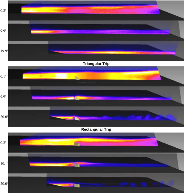
Figure 4 show several instantaneous (not time-averaged) images of hypersonic boundary layer flow passing over the flat plate with and without trips. All images shown were acquired on the centerline, directly downstream of the four NO seeding ports. Several comments should be made regarding these PLIF images. The PLIF images are shown in false color, with blue, red and yellow qualitatively indicating low, medium, and high concentration of NO, respectively. Based on past experience using PLIF to study transition,19 steady, smooth PLIF images are associated with laminar flow while unsteady, jagged images are associated with transitional or turbulent flow. Slight left-to-right variations in the PLIF intensity are primarily caused by shot-to-shot variations in laser-sheet intensity but can also be caused by other effects such as temperature variations. These should not necessarily be interpreted as NO concentration variations except when dramatic changes of intensity occur. However, vertical variations in PLIF intensity are generally significant and primarily indicate the NO distribution. The location of the trip is more than 20 injection-port diameters downstream of injection. Thus, we assume that the NO mixes well into the boundary layer fluid downstream of the injection ports. This assumption is substantiated by the images, in which the fluorescence appears relatively uniform forward of the trips. Furthermore, we believe that the NO fluorescence marks the boundary layer fluid since the masses of NO and air are very similar and also since the Lewis number (ratio of the thermal diffusivity to the mass diffusivity) is nearly unity. Thus, the fluorescence images can be thought of as images of the boundary-layer fluid.
In each of the ViDI renderings, the position of the virtual camera is fixed relative to, and raised slightly above, the flat plate so that the flat plate does not appear to move during an angle-of-attack sweep. This arrangement was chosen to deemphasize the motion of the flat plate and also to facilitate comparison of the images with one another. Furthermore, the parts of the PLIF images not containing fluorescence have been made nearly transparent during the ViDI processing. These areas appear in the ViDI renderings as light gray areas identifying the boundary of the imaged region. The area imaged by the camera, which is fixed in space, appears to shift in the ViDI renderings as the flat plate angle varies.
Flat Plate Angle δ θ Me Reθ Reθ/ Me k/δ
0° 3.94 mm 0.155 mm 7.67 300 39.2 0.51
10° 1.52 mm 0.107 mm 5.21 286 54.8 1.32
20° 1.06 mm 0.102 mm 3.85 309 80.4 1.89
Table 2. Results of laminar CFD computations for the hypersonic flow over the flat plate in the nominally Mach 10 wind tunnel. All properties are reported at the location of the trip, which was a distance of 92.1 mm downstream of the sharp leading edge.
American Institute of Aeronautics and Astronautics 7
B. Overview of Flow Characteristics for Variations in Flat Plate Angle and Trip Geometry
In the top three panels of Figure 4, when there is no trip inserted into the wedge, the flowfield remains smooth and steady as the angle of the flat plate is changed from 0º to 20º. We interpret this to be laminar flow. Furthermore, a 0º flat plate angle produced flows that were laminar for all cases (with and without trips). At 0º flat plate angle, the boundary layer thickness, as visualized by the NO, was thicker than at the other two angles: it is
No Trip 0.2º 9.9º 19.9º Triangular Trip 0.1º 9.9º 20.0º Rectangular Trip 0.2º 10.1º 20.0º
Figure 4. PLIF images of the boundary layer flow with no trip, triangular trips and rectangular trips at the flat plate angles indicated on the left of each image. All images were acquired on the model centerline. The virtual camera used to produce these ViDI images has been affixed to the reference frame of the flat plate to deemphasize the model’s motion. The distance from the trip to the end of the flat plate is about 65 mm or 2.5”.
American Institute of Aeronautics and Astronautics 8
roughly double the height of the trips. This thicker boundary layer is caused by the lower Reynolds number and higher Mach number at this angle of attack.
When the height of the triangular trip is comparable to the boundary layer thickness (which occurs at a flat plate angle of ~10º), the boundary layer still appears to remain laminar, as seen in Fig. 4. In this image, the gas skips past the triangle and appears to maintain a uniform distribution of NO, similar to the 0º case. However, examination of many such images at this condition shows that the flow experiences some instability at this condition, occasionally transitioning to turbulence, particularly well downstream of the trip. Thus, at this angle, the flow is unstable well downstream of the trip and verging on transition to turbulence. At a 20º flat plate angle however, the flow downstream of the trip exhibits more mixing and diffusion associated with a transitioning or turbulent flow, as seen in Fig. 4. Most of the images taken at this condition showed this behavior.
In the rectangular-trip images of Fig. 4, when the boundary layer thickness is greater than the trip height, the flow remains laminar. When the boundary layer thickness is approximately equal to the height of the trip, the flow is mostly laminar but occasionally transitioning to turbulent flow. There is a key difference in the bottom panel of Fig. 4 however, where the boundary layer thickness is less than the height of the rectangular trip. In this case, the fluorescence is very bright in front of the trip, but only weak fluorescence, showing transitioning or turbulent flow, is visible downstream of the trip. In most of the images taken at this condition on the model centerline, there is no laser-induced fluorescence downstream of the trip. It appears that the flow is diverted around the trip in this case – a point that will be discussed further below.
Another observation is that the flow over the triangular trip at 0° flat plate angle closely resembles the flow with no trip, indicating that the trip is minimally perturbing the flow at this angle. However, the flow downstream of the square trip at this same flat-plate angle shows a much brighter band of fluorescence in the top half of the wake flow, indicating that more NO-seeded fluid is located there. The square trip is impacting this flow more than the triangular trip. This could be because the square trip has twice the surface area, causing twice the blockage, of the triangular trip of the same height. Similarly, at a flat plate angle of 10º, more of the rectangular-trip images were transitional than triangular-trip images – again probably because the area of the rectangular trip is larger.
-8 -4 0 4 8 12
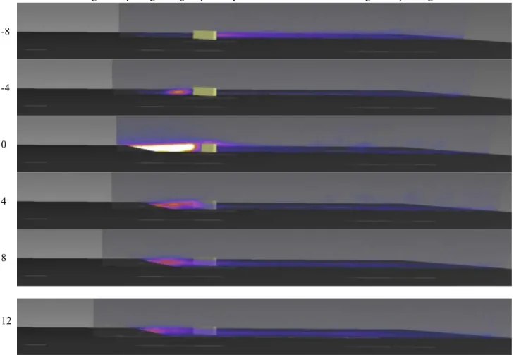
Figure 5. PLIF images of the boundary layer flow for the rectangular trips at 2020º º flat plate angle; spanwise locations (in mm) are indicated at the left of each image. Zero is the model and trip centerline, and the positive direction is defined to be toward the viewer.
American Institute of Aeronautics and Astronautics 9
C. Rectangular Trip at 20º Flat Plate Angle: Laser Sheet Scan
At a 20º flat plate angle, the laser sheet was scanned towards the ICCD camera for a total scan range of 20 mm. It was scanned from 8 mm on the far side of the centerline of the trip to 12 mm towards the camera’s side of the trip. Over the course of the scan, the flow structure varied significantly with respect to the proximity of the trip. When the laser sheet was positioned directly over the centerline of the trip (0 mm position in Fig. 5), the fluid flow was mainly being obstructed by the trip. Occasionally, small amounts of fluid flowed over the trip, resulting in a turbulent flow structure. However, most of the images obtained near the center of the rectangular trip showed no fluorescence downstream of the trip. When the laser sheet is positioned more than 6 mm on one or the other side of the centerline, as shown in the panels corresponding to -8, 8, and 12 mm in Fig. 5, continuous flow structures are observed downstream of the trip. The flow mostly diverts around the trip within the boundary layer. Since the trip was placed at a 45º angle with respect to the oncoming flow, and oriented with the camera’s side of the trip further downstream, most of the flow is observed to pass by the camera’s side of the trip. However, some flow is observed to divert to the far side of the trip as well, as evidenced by the top panel of the figure.
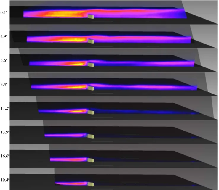
0.1º 2.9º 5.6º 8.4º 11.2º 13.9º 16.6º 19.4º
Figure 6. PLIF images of the boundary layer flow for the rectangular trips at various flat plate angles, as shown to the left of each image. All images were acquired on the model centerline.
American Institute of Aeronautics and Astronautics 10
D. Rectangular-Trip Angle-of-Attack Sweep
For part of the rectangular-trip tunnel run, the laser sheet was placed on the model centerline and the angle of attack of the model was swept from 20º to 0°. This allowed virtually continuous visualization of the growth of the boundary layer relative to the height of the trip. A total of 57 frames of data were acquired during this sweep. Figure 6 shows every 8th frame from this sequence. At the steepest flat plate angle of 20º, the boundary layer is thinner than the trip and flow is primarily diverted around the trip as shown in Fig. 5. As the angle of the plate decreases from 20º, the boundary layer in front of the trip, identified by the presence of NO, thickens. Eventually, the boundary layer grows to be thicker than the trip and wisps of NO are observed to pass over the trip. At still shallower angles, the boundary layer flows continuously over the center of the trip. Finally, at the lowest angle of attack, the flow passes directly over, engulfing the trip, while maintaining laminar flow. Curiously, all the images obtained on this angle of attack sweep appeared to show laminar-like behavior. Had the laser sheet been placed 5 mm to one side or the other of the centerline, turbulent images would probably have been observed at the higher flat plate angles, as evidenced by Fig.5. Note that the placement of the images relative to the rendered model may not be perfect during ViDI processing, so the absence of PLIF immediately in front of the trip should not necessarily be interpreted as a shock wave.
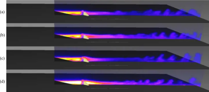
E. Triangular-Trip at 20º Flat Plate Angle: Images Showing Transition to Turbulence
Most of the images acquired for flow over the triangular trip at a 20º flat plate angle were transitioning or turbulent. In this section we present and discuss a selection of these images. Figure 7 shows that the flow immediately downstream of the trip appears to be smooth and laminar. Then the boundary layer oscillates before breaking down into turbulent eddies. Curiously, within each image, the shape of, and spacing between these structures is somewhat regular, indicating that a periodic instability is creating these structures. These images are consistent with a Kelvin-Helmholtz type instability forming in the shearlayer just downstream of the trip. This instability forms a wavy structure that rolls up into an eddy. The structures on the right side of the images are typically 5-7 mm apart and in many cases the structures are completely separated from each other – unseeded air having been mixed into the boundary layer. Another observation is that the turbulent flow structures protrude well out of the boundary layer. Turbulent structures are observed that are twice as tall as the laminar boundary layer would have been, in the absence of the trips due to the thickening of the turbulent boundary layer.
(a)
(b)
(c)
(d)
Figure 7. Single-shot PLIF images of the boundary layer flow over the triangular trip at a flat plate angle of 20º, all exhibiting turbulent flow. All images were acquired on or very near to the model centerline.
American Institute of Aeronautics and Astronautics 11
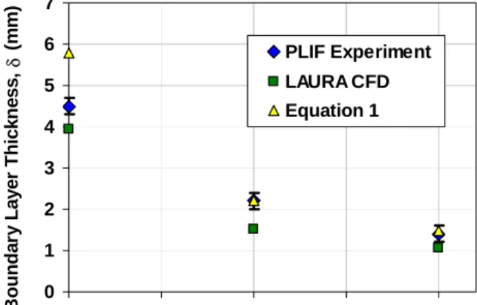
F. Comparison of Experimentally-Measured Boundary Layer Thickness with Computations
As mentioned above, the NO seeded into the boundary layer near the flat plate’s leading edge mixes with the boundary layer fluid, marking the boundary layer further downstream. An experimental measurement of the boundary layer thickness can be approximated from these images. Optical filters were used to reject the laser scattered light at the surface of the model, so the
location of the flat plate in the PLIF images is difficult to determine accurately. We instead based the measured boundary layer thickness directly on the visible thickness of the PLIF intensity in the direction normal to the boundary layer. The bottom of the boundary layer, adjacent to the plate, was determined from the location in the image where the PLIF intensity was half the maximum value within the boundary layer. Similarly, the top of the boundary layer was determined by the location, furthest away from and perpendicular to the plate, where the intensity was half of its maximum. This choice of boundary was arbitrary. A thickness based on 10% of the maximum PLIF signal at the top of the boundary layer could alternately have been used, for example, resulting in a 20% thicker estimate of the boundary layer thickness, on average. The relationship between PLIF intensity and NO concentration is complicated,20 and future work should investigate the relationship between NO PLIF intensity, NO concentration, and the boundary layer thickness, δ, based on conventional criteria. Comparisons of the boundary layer thicknesses from PLIF, CFD and Equation 1 are presented in Figure 8.
The boundary layer thickness decreases as the flat-plate angle increases for both the experiment and the theoretical predictions, as described previously. The experiment and Eq. 1 agree for 10° and 20° flat plate angles. This agreement is probably fortuitous, considering the assumptions, discussed above, that were made in computing these thicknesses. The lack of agreement at a zero degree angle of the flat plat is not surprising: the use of Eq. 1 entirely neglected the viscous interaction effect near the leading edge which significantly decreases the Mach number at this flat plate angle. The viscous interaction effect is less significant as the flat-plate angle increases. The CFD-predicted boundary layer thicknesses are smaller than the measured thicknesses by 12-31% (about 0.3-0.7 mm). Discrepancies between these thicknesses could be either caused by uncertainties in the conditions used to compute the CFD, assumptions made in setting up the CFD, or the fact that these two boundary layer thicknesses are defined differently. Nonetheless, the similar magnitudes and trends in the measured and calculated boundary layer thicknesses provide evidence that NO PLIF is marking the boundary layer fluid, which aids in qualitative interpretation of the images.
G. Comparison with Orbiter Return-to-Flight Transition Studies
It is worthwhile to compare the results obtained in this experiment with past work to determine whether transition to turbulence observed with PLIF correlates with transition to turbulence observed by other means. In Fig. 9, the two right columns from Table 2 are plotted against each other, since these are parameters used in Ref. 2 to predict transition to turbulence. NASA developed the empirically-based boundary layer transition (BLT) tool for predicting whether and when the boundary layer flow over the windward surface of the Space Shuttle Orbiter will transition into a turbulent flow as a function of location and size of any damaged regions of the vehicle.2 Wind tunnel data used to develop this tool was obtained using the phosphor thermography technique, which provides global surface heating images.21 As described above, the BLT tool is part of a suite of tools used to assess whether necessary steps, including repairs, should be taken to ensure the safe reentry of the vehicle. Figure 9 shows how the transition parameterReθ/Me and disturbance parameterk/δ are related.2 The red curve is given by the equation:
(Reθ/Me) (k/δ) = C, (2) 0 1 2 3 4 5 6 7 0 5 10 15 20
Flat Plate Angle (degrees)
B o u n d a ry L a ye r T h ic kn es s, δ ( mm) PLIF Experiment LAURA CFD Equation 1
Figure 8. Comparison of measured and calculated boundary layer thicknesses. Measurements were taken 92 mm downstream of the leading edge of the flat plate (the location of the trip) on the run with no trip inserted. Error bars of ±0.2 mm indicate the uncertainty in the measurement, which are based on frame-to-frame height variations as well as uncertainty in the measurement method.
American Institute of Aeronautics and Astronautics 12
where C is called the curve coefficient. As noted in Ref. 2 transition results from the 20-In Mach 6 Tunnel offered the most reliable transition onset predictions when compared to flight Orbiter calibration cases, yielding a conservative curve coefficient of C=27. Points falling below this curve correspond to laminar flows while points falling above the curve correspond to transitional or turbulent flows. Note, however, that the correlation curve shown in Fig. 9 was based on the LATCH engineering code which was chosen because of its fast computational speed, and not LAURA, which has higher fidelity.2
When the model is at a 20º flat plate angle, Reθ/Me≈ 80 and k/δ≈ 1.9: the corresponding flow is
predicted by the curve in Fig. 9 to be turbulent. This agrees with our measurements for both types of trips. When the model is at a 0º flat plate angle, Reθ/Me ≈
39 and k/δ≈ 0.5 the data point falls below the line, indicating that the flow remains laminar. Again, this agrees with PLIF images obtained at that condition, for both trips. When the model is at a flat-plate angle of 10º, Reθ/Me ≈ 55 and k/δ ≈ 1.3, the flow is
predicted to be transitional or turbulent. However in our experiment, we observe that flow is sometimes laminar and sometimes transitional for both trips at these conditions. Considering that the curve coefficient is a conservative predictor of transition onset, our measurements are consistent with the correlation used for the Shuttle Orbiter RTF program.
Still, comparisons between the present set of experimental data and curve coefficients determined in past work should be made with caution. There are potentially significant issues affecting such
comparisons. First, our PLIF observations were limited to a distance of ~30 trip heights downstream of the trip, compared to 400-2000 trip heights observed in Ref. 21, which was used to generate the curve coefficient discussed in Ref. 2. If the flat plate were longer (or the trips shorter and boundary layer thinner), more fully developed turbulent flow may have been observed for the 10º flat-plate angle, for example. Another possible source of concern in making comparison is that the prior experimental work used trips that were a different shape than the present trips. The trips used in this past work were the shape of slightly-protruding shuttle tiles, not protruding gap filler material used in the present study. The gap filler is significantly thinner (relative to its height) in the direction of the flow than raised shuttle tiles. Furthermore, previous work indicates that transition length depends on the shape of passive trips,4 whereas the BLT presently does not account for differences in trip shape or orientation.2 So, caution should be exercised when comparing such data sets.
V. Discussion of Prospects for Continuation of Related Work
With the current (or similar) apparatus, it would be possible to perform a series of experiments with different trip heights and different tunnel Reynolds numbers to develop a new curve coefficient for these gap-filler shaped trips. Such measurements could be corroborated by heat flux data to confirm interpretation of the images. The use of angle-of attack sweeps during a single tunnel run means that many combinations of Reθ/Me ≈ 27 and k/δ can be
probed on each run. Thus, a parameter space could be efficiently and accurately mapped using this PLIF flow visualization technique. However, as the angle-of-attack sweep shown in Fig. 5 illustrates, turbulent flow can exist but not be visualized if the laser sheet is not imaging the region of turbulence, for example right downstream of a trip. This problem could be overcome by expanding the laser beam from a thin sheet into a sheet that is thicker than the width of the trip. Such flow visualizations would be sure to observe turbulent flow downstream of the trip, if it exists. However, additional laser energy might be required in order to perform this type of flow visualization.
An unfortunate artifact of the present experiment is that the injection of NO through four small diameter ports upstream of the trip is a classic “jet in a cross flow,” which introduces vorticity into the flow, thereby destabilizing the boundary layer.4 In fact, images obtained in this experiment but not presented in this paper show evidence of a pair of weak counter-rotating vortices forming well downstream of the injection, near the aft end of the flat plate. In
0 20 40 60 80 100 120 140 0 0.5 1 1.5 2 2.5 k/δ Reθ /M e 0 degree, Laminar 10 degree, Transitional 20 degree, Turbulent C = 27
Figure 9. Graph that predicts whether flow downstream of a trip will be laminar (below the curve) or turbulent (above the curve). The angle in the legend refers to the angle of the flat plate with respect to the oncoming flow.
American Institute of Aeronautics and Astronautics 13
the future, other strategies of seeding NO could be investigated to eliminate this undesirable artifact. For example, instead of using four small diameter tubes, as is the case in the present experiment, a large area (25mm x 25 mm or 1 inch square) insert of porous material could be used to introduce NO well upstream of the trips.4 This would decrease the velocity of the gas exiting the jets from 10-30 m/s to < 1 m/s, thereby minimizing the vorticity added to the flow. Another method for circumventing this same problem would be to perform future experiments in a facility that has naturally-occurring NO, such as a shock tunnel or an arc-heated wind tunnel. Alternatively, a tunnel operating on N2 could be uniformly seeded with NO, though this could be prohibitively expensive.
A second possible artifact that may be present in the present experiment is that the seeded NO can react with the air in the wind tunnel. This reaction is exothermic and its reaction rate increases with decreasing temperature. It has been suggested that in cold hypersonic flows this reaction can release large amounts of heat, potentially perturbing the flowfield. Future experiments and computations are planned to address this concern.
In future similar experiments, additional improvements could be made. A higher magnification optical system could be used to zoom in on the near-trip region, which was not highly resolved in the present experiment. Also, measurements could be performed with shorter trips and at higher pressure conditions in order to observe transition at further downstream locations based on number of trip heights.
VI. Conclusion
PLIF visualization of nitric oxide (NO) seeded into a boundary layer flow has been used to observe transition to turbulence in the hypersonic flow over trips. Three cases were investigated: flow over a flat plate with no trip, a triangular trip, and a rectangular trip. The trips were oriented at a 45º angle with respect to the oncoming flow. This experimental geometry was chosen to simulate protruding gap-filler material on the Space Shuttle Orbiter. The angle of attack of the flat plate was varied during the tunnel runs, causing the boundary layer thickness to change from smaller than the trip height to larger than the trip height. When the flat plate was parallel to the freestream flow, the boundary layer was found to be laminar for all three cases. When the flat plate was positioned at a 20° angle with respect to the freestream flow, the boundary layer was laminar for the case with no trip and turbulent for the tripped cases. At an intermediate flat plate angle, transitional flow was observed for the tripped cases. The qualitative identification of transition to turbulence using PLIF compared favorably with recent work in which transition was identified using other methods.
Acknowledgments
We wish to acknowledge the contribution to this project from the NASA Langley Research Center 31-Inch Mach 10 Air tunnel technicians and engineers, including Kevin Hollingsworth, Paul Tucker Tony Robbins, Henry Fitzgerald, and Johnny Ellis. Also we wish to thank Rich Schwartz of Swales Aerospace, Hampton, Virginia, for assisting with setting up and executing the ViDI analysis, and Rudy King from NASA Langley Research Center for several suggestions that improved the text and helped to interpret the images. This work was supported by the NASA Fundamental Aeronautics Hypersonics Program.
References
1S. A.Berry, T. J.Horvath, A. M. Cassady, B. S. Kirk, K.C. Wang, and A. J. Hyatt, “Boundary Layer Transition Results From STS-114,” 9th AIAA/ASME Joint Thermophysics and Heat Transfer Conference, AIAA-2006-2922, June 2006.
2 S. A. Berry, T. J. Horvath, F. A. Greene G. R. Kinder, and K. C. Wang, “Overview of Boundary Layer Transition Research in Support of Orbiter Return to Flight,” AIAA-2006-2918, 9th AIAA/ASME Joint Thermophysics and Heat Transfer Conference, June 5-8 2006, San Francisco, California.
3 C. H. Campbell, B. Anderson, G. Bourland, S. Bouslog, A. Cassady, T. Horvath, S. Berry, P. Gnoffo, B. Wood, J. Reuther, D. Driver, D .Chao, , and D. Picetti, “Orbiter Return To Flight Entry Aeroheating,” 9th AIAA/ASME Joint Thermophysics and Heat Transfer Conference, AIAA-2006-2917, June 2006.
4 S. A. Berry, R. J. Nowak, and T. J. Horvath, “Boundary Layer Control for Hypersonic Airbreathing Vehicles” 34th AIAA Fluid Dynamics Conference, Portland, Oregon AIAA-2004-2246, 28 June - 1 July, 2004.
5 P. C. Palma, S. G. Mallinson, S. B. O’Byrne, P. M. Danehy, and R. Hillier, "Temperature measurements in a hypersonic boundary layer using planar laser-induced fluorescence," AIAA Journal, Vol. 38, No. 9, p. 1769-1772, 2000.
6 M.W. Smith and A.J. Smits, “Visualization of the Structure of Supersonic Turbulent Boundary Layers,” Experiments in Fluids, 18, 288-302, 1995
7 B. Auvity, M. R. Etz, and A. J. Smits “Effects of transverse helium injection on hypersonic boundary layers,” Phys. Fluids, Vol. 13, No. 10, p. 3025-3032, October 2001.
American Institute of Aeronautics and Astronautics 14
8 S. O’Byrne, P. M. Danehy, A. F. P. Houwing, Investigation of hypersonic nozzle flow uniformity using NO fluorescence, Shock Waves Journal, May, Pages 1 - 7, DOI 10.1007/s00193-006-0013-6, URL http://dx.doi.org/10.1007/s00193-006-0013-6 (2006); P. C. Palma, P. M. Danehy, A. F. P. Houwing, "Fluorescence Imaging of Rotational and Vibrational Temperature in a Shock Tunnel Nozzle Flow," AIAA Journal, Vol. 41, no. 9, Sept. p. 1722-1732, 2003; M.J. Gaston, A.F.P. Houwing, N.R. Mudford, P.M. Danehy, J.S. Fox, “Fluorescence imaging of mixing flowfields and comparisons with computational fluid dynamic simulations” Shock Waves Journal v. 12, n. 2, p. 99-110, 2002; P. M. Danehy; P. Mere; M. J. Gaston; S. O'Byrne; P. C. Palma; A. F. P. Houwing “Fluorescence Velocimetry of the Hypersonic, Separated Flow over a Cone,” AIAA Journal, v. 39(7), p. 1320-1328, 2001; J. S. Fox; S. O'Byrne; A. F. P. Houwing; A. Papinniemi; P. M. Danehy; N. R. Mudford, “Fluorescence Visualization of Hypersonic Flow Establishment over a Blunt Fin,” AIAA Journal, v. 39(7), p. 1329-1337, 2001.
9 P. M. Danehy, J. A. Wilkes, G. Brauckmann, D. W. Alderfer, S. B. Jones, and D. Patry, “Visualization of a Capsule Entry Vehicle Reaction-Control System (RCS) Thruster” AIAA Paper 2006-1532 44th AIAA Aerospace Sciences Meeting and Exhibit, Reno, Nevada, Jan. 9-12, 2006.
10 P. M. Danehy, J. A. Wilkes, D. W. Alderfer, S. B. Jones, A. W. Robbins, D. P. Patry and R. J. Schwartz “Planar laser-induced fluorescence (PLIF) investigation of hypersonic flowfields in a Mach 10 wind tunnel” AIAA AMT-GT Technology Conference, San Francisco, AIAA-2006-3442 June 5-8, 2006.
11 S.G. Mallinson, S.L. GAI, and N.R. Mudford, “The boundary layer on a flat plate in hypervelocity flow,” Aeronautical Jouurnal, April 1996.
12 J. A. Wilkes, D. W. Alderfer, S. B. Jones, and P. M. Danehy, “Portable Fluorescence Imaging System for Hypersonic Flow Facilities,” JANNAF Interagency Propulsion Committee Meeting, Colorado Springs, Colorado, December 2003.
13 J. R. Micol “Langley Aerothermodynamic Facilities Complex: Enhancements and Testing Capabilities,” AIAA Paper 98-0147, 36th AIAA Aerospace Sciences Meeting & Exhibit, January 12-15, Reno, NV, 1998.
14 D.W. Alderfer , P.M. Danehy , S.E. Borg , J.A. Wilkes , K.T. Berger , G.M. Buck, and R. J. Schwartz, “Fluorescence Visualization of Hypersonic Flow Over Rapid Prototype Wind-Tunnel Models” AIAA Paper 2007-1063 45th AIAA Aerospace Sciences Meeting and Exhibit, Reno, Nevada, Jan. 8-11, 2007.
15 Schwartz, R.J., "ViDI: Virtual Diagnostics Interface Volume 1-The Future of Wind Tunnel Testing" Contractor Report NASA/CR-2003-212667, December 2003
16 Autodesk 3ds Max Product Information, Autodesk Inc.,
http://usa.autodesk.com/adsk/servlet/index?id=5659302&siteID=123112, viewed Jan 2, 2006.
17 Cheatwood, F.M., Gnoffo, P.A., “User’s Manual for the Langley Aerothermodynamic Upwind Relaxation Algorithm (LAURA)”, NASA TM 4674, April 1996.
18 Gnoffo, P.A, Gupta, R. N., “Conservation Equations and Physical Models for Hypersonic Air Flows in Thermal and Chemical Nonequilibrium”, NASA Technical Paper 2867, February 1989.
19 J. A. Wilkes, P. M. Danehy, and R. J. Nowak, "Fluorescence Imaging Study of Transition in Underexpanded Free Jets" 21st International Congress on Instrumentation in Aerospace Simulation Facilities, Sendai, Japan, Aug. 29-Sept. 1, 2005.
20 Eckbreth, A. C., Laser Diagnostics for Combustion Temperature and Species, 2nd ed., Gordon and Breach Publishers, The Netherlands (Oct 1996).
21 D. S. Liechty, S. A. Berry, and T. J. Horvath “Shuttle Return To Flight Experimental Results: Protuberance Effects on Boundary Layer Transition”, NASA/TM-2006-214306, June 2006.