Factor Models and Dynamic Stochastic General Equilibrium models: a forecasting evaluation

(1)

University LUISS “Guido Carli”

of Rome

Ph.D Program in Economics (XXIV Cycle)

Factor Models and Dynamic

Stochastic General Equilibrium

models: a forecasting evaluation

Gabriele Palmegiani a.y. 2011/2012

Advisor: Prof. Marco Lippi

(2)

Abstract

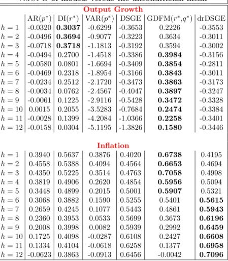
This dissertation aims to put dynamic stochastic general equilibrium (DSGE) fore-casts in competition with factor models (FM) forefore-casts considering both static and dynamic factor models as well as regular and hybrid DSGE models. The empir-ical study shows three main conclusions. First, DSGE models are significantly outperformed by the generalized dynamic factor model (GDFM) in forecasting output growth in both short and long run, while the diffusion index (DI) model outperforms significantly DSGE models only in the short run. Second, the most surprising result of the dissertation, we discovered that only the hybrid DSGE model outperforms significantly all other competitive models in forecasting infla-tion in the long run. This evidence falls out with recent papers that found just regular DSGE models able to generate significant better forecasts for inflation in the long run as well as papers where hybrid DSGE models are found to forecast poorly. Third, in most cases, the unrestricted vector autoregressive (VAR) model represents the worse forecasting model. Although our results are consistent with the prevalent literature who gives to factor models the role to forecast output vari-ables and to DSGE models the role to forecast monetary and financial varivari-ables, this research documents that exploiting more information on many macroeconomic time series, through hybrid DSGE models, is important not only to obtain more accurate estimates, but also to get significantly better forecasts.

Keywords: Diffusion Index (DI) model, Generalized Dynamic Factor Model (GDFM), Dynamic General Equilibrium (DSGE) model, Data-Rich DSGE (drDSGE) model, Equal Predictive Ability Tests.

(3)

Introduction

Recent years have seen rapid growth in the availability of economic data. Statisticians,

economists and econometricians now have easy access to data on many hundreds of variables

that provide the information about the state of the economy. Coinciding with this growth

in available data, two main new econometric models that exploit this wider information have

been proposed: the factor models (FM) and the Dynamic Stochastic General Equilibrium

(DSGE) models. Factor models have been successfully applied when we have to deal with:

construction of economic indicators (Altissimo et al. (2010)), business cycle analysis (Gregory

et al. (1997) and Inklaar et al. (2003)), forecasting (Stock and Watson (2002a,b) and Forni et

al. (2000)), monetary policy (Bernanke and Boivin (2003) and Bernanke et al. (2005)), stock

market returns (Ludvigson and Ng (2007)) and interest rates (Lippi and Thornton (2004)).

DSGE models have been successfully applied when we have to deal with: forecasting (Smets

and Wouters (2002) and Smets and Wouters (2007)), estimation accurancy (Boivin and

Gian-noni (2006) and Kryshko (2009)), credit and banking (Gerali et al. (2008)), interest term of

structure analysis (Amisano and Tristani (2010)) and monetary policy (Boivin and Giannoni

(2008)).

Among all these applications, the recent economic global crisis has pointed out how

fore-casting well is central. For this reason, the main objective of this dissertation is to provide

a detailed forecasting evaluation between these two econometric models taking into account

of the recent developments in both factor and DSGE modelling. The novel of this research is

the expanded range of forecasting models treated. Infact, our forecasting competition

consid-ers not only static factor models and regular DSGE models but also dynamic factor models,

such as, the so-called Generalized Dynamic Factor Model (GDFM) of Forni et al. (2000) and

hybrid DSGE models, such as, the so-called Data-Rich DSGE (drDSGE) following Boivin

(6)

although there are some forecasting discussions on both dynamic factor model and regular

DSGE individually, there is no attempt in the literature, to carry out a strong forecasting

evaluation between dynamic factor models and hybrid DSGE models. In particular, what is

missing is a forecasting comparison between the GDFM and the drDSGE.

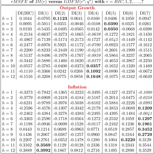
The empirical study shows three main conclusions. First, DSGE models are significantly

outperformed by the GDFM in forecasting output growth in both short and long run, while

the static factor model outperforms significantly DSGE models only in the short run. Second,

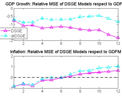
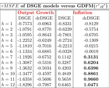
the most surprising result of the dissertation, we discovered that only the drDSGE

outper-forms significantly all other competitive models in forecasting inflation in the long run. This

evidence falls out with both Wang (2009) who found that a regular DSGE was able to generate

significant better forecasts for inflation in the long run, and Paccagnini (2011) where hybrid

models are found to forecast poorly. Therefore, the drDSGE outperforms significantly the

reg-ular DSGE in forecasting both output growth and inflation, confirming that exploiting more

information on many macroeconomic time series, through the drDSGE, is important not only

to obtain more accurate estimates, but also to get significant better forecasts. Third, in most

cases, the unrestricted VAR is outperformed by the unconditional mean of the time series of

interest, confirming that this model should not be used as benchmark model in forecasting

comparisons.

This work is closely related with Wang (2009), but while we share some of the features

of his study, our analysis is greatly expanded. First, we do not use the simple DSGE model

of Del Negro and Schorfheide (2004) but the most elaborated DSGE model of Smets and

Wouters (2007). Second, among factor models, we considered also the GDFM of Forni et

al. (2000) whose forecasting performance is documented to be superior than the static factor

model of Stock and Watson (2002a,b). Third, among DSGE models, we put side by side the

regular DSGE model of Smets and Wouters (2007) with its representation in terms of drDSGE

following Boivin and Giannoni (2006) and Kryshko (2009). Therefore, our work is also

re-lated with the fast growing literature in both factor models and DSGE models. About factor

models, Forni et al. (2000) have presented and estimated their GDFM using a two-sised filter

of the observations, Stock and Watson (2002a) have introduced their diffusion index model

demostrating its ability to outperform autoregressions and small vector autoregressions

fore-casts, Stock and Watson (2002b) have shown the asymptotically efficiency of static principal

(7)

Soggetta a copyright. Sono comunque fatti salvi i diritti dell’Università LUISS Guido Carli di riproduzione per scopi di ricerca ec didattici, con citazione della fonte.

static factors under a diffusion index model, Forni et. al. (2005) have proposed a refinement

of their two-sided filter into a one-sided filter to allow forecasting feasible, Forni et al. (2009)

have emphasized how identification schemes in strustural VAR analysis can be adapted in

their GDFM, while Stock and Watson (2010) have described in great detail dynamic factor

models. About DSGE models, Smets and Wouters (2007) have extended their previous DSGE

model allowing more structural shocks and more financial frictions confirming that the DSGE

model has a fit comparable to that of bayesian vector autoregression (BVAR) models, Del

Negro et al. (2004) and Del Negro et al. (2007) have shown that a relatively simply DSGE

model employed as a prior in a VAR is able to improve the forecasting performance of the VAR

relative to an unrestricted VAR or a Bayesian VAR, Rubaszek and Skrzypczynski (2008) have

emphasized how DSGE model forecasts are poor in forecasting inflation and interest rates in

short term, Christoffel et al. (2010) have pointed out that large bayesian VAR can outperfom

DSGE forecasts, while Edge et al. (2011) have shown how their DSGE model can forecast

poorly inflation and output growth.

The dissertation is organized followingFigure (1.1). Given a large data-set, indeed a data-set

Figure 1.1: The dissertation path.

with many economic time series variables, we evaluate the forecasting performance of factor

models relatively to the DSGE models passing through: identification, estimation,

fore-casting and forecasting inference. We open discussing the identification and estimation

schemes of both factor models(Chapter (2)) and DSGE models (Chapter (3)). In particular,

Chapter (2)describes the identification and the estimation of both static and dynamic factor

models with a special focus to the recent identification and estimation scheme proposed by

Forni and Lippi (2001) of their so-called Generalized Dynamic Factor Model (GDFM), while

(8)

mo-tivating the advantages of using its Data-Rich Environment version. Estimated the models,

we move on forecasting and forecasting inference (Chapter (4)). The forecasting step

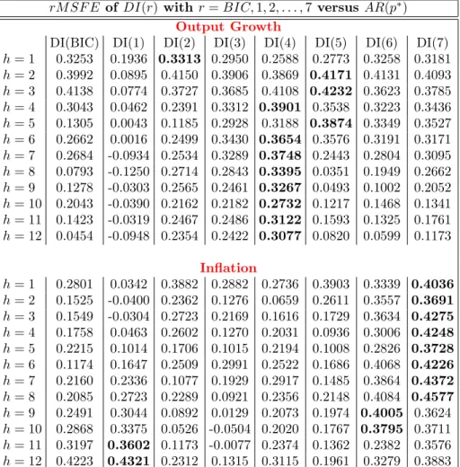
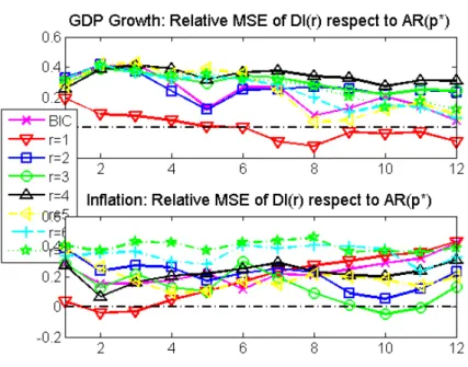
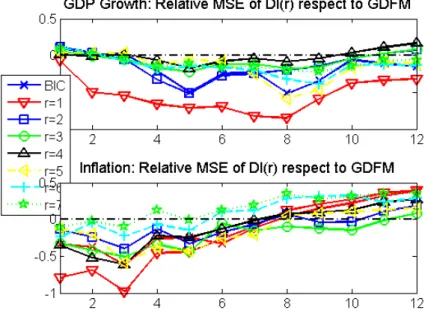
eval-uates the models forecasting performance through the relative mean squared forecast error

(rM SF E) metric, defined as:

rM SF E(m, n)|h= 1−

M SF Em|h

M SF En|h

whereM SF Em|h and M SF En|h denote respectively the mean squared forecast error

gener-ated from modelm at the forecasting horizion h and the mean squared forecast error

gener-ated from modelnat the forecasting horizion h. TherM SF E(m, n)|h can be interpreted as

a forecasting gain of modelm relative to the modelnat the forecasting horizionh when it is

positive, or it can be interpreted as a forecasting loss of the model m relative to the model

n at the forecasting horizion h when it is negative. In other words, the rM SF E(m, n)|h

answers to the question: ...between modelm and n, which model should be used to forecast

a given time seriesh steps ahead? This metric represents an appropriate tool to measure the

forecasting perfomance of DSGE models as documented by Smets and Wouters (2003), Smets

and Wouters (2007), Edge et al. (2010) and Edge et al. (2011).

As pointed out by Diebold and Mariano (1995) and West (1996) and Giacomini and White

(2006), the main drawback of this M SF Eanalysis is the lack of significance, indeed it is not

possible to make rigorous statistical statements by simply interpreting the observed differences

betweenM SF Esbecause any metric has not a significance power. We need to look into model

forecasting inference. We use two test of forecasting accurancy: the test of equal unconditional

predictive ability of Diebold and Mariano (1995) and West (1996) (hereafter DMW test), and

the test of equal conditional predictive ability of Giacomini and White (2006) (heafter GW

test). Since, as shown by Clark and McCracken (2001), the unconditional test has low power

in the finite sample, particularly when nested models are involved, the final results of the

(9)

Chapter 2

Factor models

“All models are wrong, but some are useful” George Box

This chapter presents the identification and the estimation schemes of the factor models used

in the out-of-sample forecasting experiments. A factor model is an econometric model where each observed time series variable xit is assumed to be linearly decomposed into two

un-observed orthogonal components, the common component χit driven by a small number of

common shocks uit, and the idiosyncratic component ξit who accounts for the residual of

that decomposition. The common component is responsable of the co-movement of the series,

while the idiosyncratic component is responsable to the specific time series variation. Both

the common and the idiosyncratic component are unobserved and need to be consistently

estimated.

The chapter is organized as follows. In Section (2.1) we start considering the

identifica-tion and the estimaidentifica-tion of the Generalized Dynamic Factor Model (GDFM). InSection (2.2)

we present the identification and the estimation of the static factor model or diffusion index

(DI) model, as special case of the GDFM. In Section (2.3) we describe the one-sided

esti-mation and forecasting of the GDFM. In Section (2.4) we face the problem of determining

the number of factors, while Section (2.5) concludes discussing the link between static factor

model and the GDFM.

2.1 The generalized dynamic factor model

The Generalized Dynamic Factor model (GDFM) is a factor model that differs from theexact factor model, in which the idiosyncratic components are mutually uncorrelated, because it allows the idiosyncratic shocks to be weakly serial and cross-sectional correlated. It combines

(10)

the so-called approximate static factor model of Chamberlain and Rothschild (1983), widely applied in financial econometrics, and thedynamic factor model of Geweke (1977) and Sargent and Sims (1977) for which respectively cross-sectional and serial correlation was allowed. The

model is called dynamic since the common shocks may not impact a series simultaneously, as in the static factor model, but they can propagate with leads or lags. Then, the model

is called generalized since the common components are derived assuming a dataset with an infinite number of series and an infinite number of observations.

To setting up the model, let’s introduce the notation. Let P = (Ω,I, P) be a probability model and letL2(P,C)be the linear space of all complex-valued, zero mean, square-integrable random variables defined on Ω. Let x = {xit, i ∈ N, t ∈ Z} be the infinite double sequence of random variables defined onxit∈L2(P,C) and let xN t= (x1t, x2t, . . . , xN t)0 be the finite

N-dimensional column vector for the observation made at timet. IfPis a complex matrix we

denoteP0 as the transpose ofPandP∗ as the complex conjugate ofP0. Withθwe denote the

real interval[−π, π]. Then, given the subsetG⊆L2(P,C), we denote the closed span ofGas

span(G)which is the minimum closed subspace ofL2(P,C)containingG. IfS is a closed lin-ear subspace ofL2(P,C)andx⊆L2(P,C), we denoteproj(x|S)as the orthogonal projection ofxonS. Therefore, we denote withΣx(θ)the spectral density matrix of the double sequence

x = {xit, i ∈ N, t ∈ Z} as function of the frequencies in θ ∈ [−π, π], while with ΣxN(θ) we

denotes the spectral density matrix of theN-dimensional vector xN t= (x1t, x2t, . . . , xN t)0 as

function of the frequencies inθ∈[−π, π]. Thei-th largest eigenvalue ofΣx_N(θ), is denoted by

λx_{N i}, while the i-th largest eigenvalue of Σx(θ) is denoted by λx_i(θ). We denote the spectral

density matrices of the common and the idiosyncratic componenents and their eigenvalues in

a similar way.

We assume that for any N ∈ _N the process xN t is covariance stationary, that is, it has

finite variance-covariance matrix: E[xN tx0_N_;_t−k] =ΓxN k and spectral densityΣxN with entries

σij bounded in modulus: Γx_{N k} = 1 2π Z π −π eikθΣx_N(θ)dθ Σx_N = 1 2π +∞ X k=−∞ eikθΓx_{N k}

(11)

The generalized dynamic factor model

where the spectral density matrix can be estimated applying the discrete Fourier transform

to the sample covariance matrix.

Given these assumptions the model proposed by Forni and Lippi (2001) can be defined as

following.

Definition 2.1.1 The Generalized Dynamic Factor Model: Let q be a nonnegative integer. The double infinite sequence x = {xit, i ∈ N, t ∈ Z} is a q-dynamic factor se-quence if L2(P,C) contains an orthonormal q-dimensional white noise vector process u = {(u1t, u2t, . . . , uqt)0;t∈Z}={ut, t∈Z} and the double sequence ξ ={ξit, i∈N, t∈Z} such that: 1. For any i∈_N: xt = χt+ξt (2.1) χt = b1(L)uit+. . .+bq(L)uqt= q X j=1 b_j(L)ujt =B(L)ut (2.2)

where B(L) =b₁(L) +. . .+b_q(L) represents the lag polynominal of order q with b_i ∈

Lq₂(θ;C) for any i∈N andj= 1,2, . . . , q (or alternatively each entrybij ∈L2(θ,C) for any i∈_N andj= 1; 2;. . .;q).

2. For anyi∈N, j= 1,2, . . . , q andk∈Z, we have ξit⊥uj;t−k, then ξi;t⊥χs;t−k for any

i∈_N,s∈_N andk∈_Z.

3. ξ is idiosyncratic.

4. Puttingχ={χit, i∈N, t∈Z},λχq(θ) =∞ almost everywhere in θ.

where: χt and ξt are referred as the vector of common component and the vector of the

idiosyncratic component of xt, whileutis referred to as the vector of common shocks.

The corrisponding model in vector form is:

xN;t = χN t+ξN t (2.3)

= B_N(L)ut+ξN t

(12)

Example 2.1 One dynamic factor GDFM

Let xit be the time seriesx at thei-th cross-sectional unit with i= 1,2, . . . , N, and at time t

witht= 1,2, . . . , T. Stating thatxit admits a generalized dynamic factor model representation

with one dynamic factor, means decomposing the series as:

xit = χit+ξit (2.4)

χi;t = b1i(L)u1t+b2t(L)u2t+. . .+bqi(L)uqt

where: χit is the common component, and ξit is the idiosyncratic component. The common

component is costructed with q unobserved common shocks or dynamic factors ujt for any

j= 1,2, . . . , q that are loaded with the filters bji(L) with leads and/or lags.

2.1.1 The identification of the GDFM

The GDFM model defined inEquation (2.1) must be identified. Identification means to find

conditions on the variance-covariance of the dataxtfor which the commonχtand idiosyncratic

component ξt are identified. Following Forni et al. (2000), we need to place conditions on

the spectral density matrix of the data xt, indeed on Σx(θ), under which the common and

idiosyncratic components are identified asN goes to infinity.

Assumption 2.1 Given the double sequence x = {xit, i ∈ N, t ∈ Z} where xit ∈ L2(P,C) and given the form:

xt = χt+ξt

= B(L)ut+ξt (2.5)

we assume that:

i) the q-dimensional vector process u = {(u1t, u2t, . . . , uqt)0, t ∈ Z} is an orthonormal white noise. That is, _E[ujt] = 0 and VAR[ujt] =E[ujtu0jt] = 1 for any j and t; ujt⊥uj;t−k

for any j,t, and k6= 0;ujt⊥us;t−k for any s6=j, tand k.

ii) ξ={ξit, i∈N, t∈Z} is the double sequence such that,ξn={(ξ1t, ξ2t, . . . , ξN t)0, t∈Z} is a zero-mean stationary vector process for anyN, and ξit⊥uj;t−k for any i, j, t, k;

(13)

The generalized dynamic factor model

i∈_Nand j= 1,2, . . . , q.

This assumption has two implications. First, it implies that the vector x = {xit, i ∈N, t ∈ Z} where xit ∈ L2(P,C) is stationary and zero-mean for any N. Second, it implies that the spectral density of the N-dimensional vector xN, indeed Σx_N(θ), can be written as the

sum of the spectral density of the common component Σχ_N(θ) and the spectral density of

the idiosyncratic component Σξ_N(θ). These matrices are unobserved, then to obtain their

consistent estimation we need further assumptions.

Assumption 2.2 For any i ∈ _N, there exist a real ci > 0 such that σii(θ) ≤ ci for any

θ∈[−π, π].

Assumption 2.3 The first idiosyncratic dynamic eigenvalues λξ_N₁ is uniformly bounded. That is, there exist a real Λ such that λξ_N₁(θ) for any θ∈[−π;π]and N ∈N.

Assumption 2.4 The first q common dynamic eigenvalues diverge almost everywhere in [−π, π]. That is limn→∞λχ_{N j}(0) =∞ for j≤q, almost everywhere in [−π, π].

The Assumption 2.2 implies that all the entries σij(θ) of ΣxN(θ) are bounded in modulus,

Assumption 2.3 implies that the dynamic eigenvalues of the idiosyncratic components have

effects concentrated on a limited number of variables, while Assumption 2.4 implies that each

common shock uij is present in infinitely many cross-sectional units with nondecreasing

im-portance.

If the Assumptions 2.1 to 2.4 are satisfied, Forni and Lippi (2001) show that the double

sequence x = {xit, i ∈ N, t ∈Z} is a generalized dynamic factor model, or better, is a

q-generalized dynamic factor model.

2.1.2 Recovering the Common Components in the GDFM

Defined and identified the model, we briefly review this estimation method proposed by Forni

et al. (2000) to recovering consistently the common componentχt inEquation (2.1) starting

from the finiteN-dimensional processxN t= (xit, x2t, . . . , xN t)0. The idea is to be aware that

for the the spectral density matrix of the finite processxN t, indeedΣxN, there existN vectors

of complex-valued functions:

(14)

for j= 1,2, . . . , N such that:

a) pN j(θ) is the row eigenvector of ΣxN(θ), that is:

pN j(θ)ΣxN =λxN j(θ)pN j(θ) for any θ∈[−π, π] (2.6)

b) |pN j(θ)|2 = 1 for anyj and θ∈[−π, π];

c) pN j(θ)p∗_{N s}(θ) = 0 for anyj 6=sand anyθ∈[−π, π];

d) pN j(θ) isθ-measurable on[−π, π].

Point a) tell us simply that the pN j(θ) for any j = 1,2, . . . , N are the eigenvectors

associ-ated to the eigenvaluesλx_{N j}(θ). These eigenvalues and eigenvectors are calleddynamic, since they come from spectral eigenvalue decomposition (Equation (2.6))and not longer from the

contemporaneous variance-covariance matrix decomposition. Point b) affirms that dynamic

eigenvectors have unitary length, point c) states that dynamic eigenvectors are orthogonal,

while point d) affirms that the dynamic eigenvectors are functions misurable on the interval

[−π, π].

As consequence of properties a) to d) each dynamic eigenvector pN j(θ) can be expanded

as Fourier Series: pN j(θ) = 1 2π ∞ X k=−∞ [ Z π −π pN j(θ)eikθdθ]e−ikθ (2.7)

then applying the inverse Fourier transforme to pN j we can construct a square-summable,

N-dimensional, bilateral filter in the time domain:

p_{N j}(L) = 1 2π ∞ X k=−∞ [ Z π −π pN j(θ)eikθ]Lk (2.8)

where we used the underlined notation to denotes thatp_{N j}(L)is the inverse Fourier

transfor-mation ofpN j(θ). The product of the dynamic eigenvectors times the data, indeed the scalar

process:

dpc_jt ={p

N j(L)xN t , t∈Z}

is the so-called thej-thdynamic principal component ofxN t. Notice that, dynamic principal

(15)

The static factor model

common component fromxN t, consider the minimal closed subspace ofL2(Ω, I,P)containing

the first q dynamic principal components:

U_N =span(pN j(L)xN t=dpcjt , j = 1,2, . . . , q , t∈Z) (2.9)

then by projecting the data on the minimal closed subspace containing the first q dynamic

principal components, we get theN-dimensional common component:

χit,N = proj(xit|UN)

= K_{N i}(L)xN t (2.10)

where K_{N i}(L) = p∗_N₁_,i(L)p

N1(L) +p ∗

N2,i(L)p_N₂(L). . .+p∗N q,i(L)p_{N q}(L) is the filter matrix

that extracts the finiteN or estimated common componentχit,Nfrom the finiteN-sample data

xN t. Under the Assumption 2.1 and Assumption 2.2 this projection, indeed the estimated

common component χit,N, converges to χit in mean square as N goes to infinity, indeed:

limN→∞χit,N =χit in mean square. This result shows that the common componentχit can

be recovered asymptotically from the sequence K_{N i}(L)xN t.

2.2 The static factor model

The problem with the previous estimator is that the filterK_{N i}(L)used to recover the common

component from the data is a two-sided filter. A filter istwo-sided when the observed variables are related not only with the current and past values of the factors but also with their

future values. Although this leaves unaffected the estimate of the central part of the sample,

the performance of the estimator deteriorates as we approach the end of the sample. This

deterioration makes this method not suitable for forecasting. To outperform this forecasting

problem, the literature has proposed two approaches:

• Stock and Watson (2002b) have proposed a new estimation method based on the eigen-value decomposition of the contemporaneous variance-covariance matrix of xN t rather

than its spectral eigenvalue decomposition;

• Forni et al. (2005) have proposed the one-sided version of their two-sided filter, which respect to Stock and Watson (2002b) retains the advantages of their dynamic approach,

(16)

described in Forni et al. (2000), allowing observed variables to be related only with

current and past value of the factors.

The approach of Stock and Watson (2002b) bring us to the so-called static factor model or

diffusion index model (DI model), while the approach of Forni et al. (2005) bring us to the one-sided estimation and forecasting of their generalized dynamic factor model explained in

Section (2.3).

The model is called static when the vector of factors Ft are loaded in xN t without leads

and/or lags, but just contemporaneoulsy. Although the relation betweenxN tandFtis static,

bothFt and ξt can have a proper law of motion. For example:

xN t |{z} (N×1) = ΛN |{z} (N×r) Ft |{z} (r×1) + ξN t |{z} (N×1) (2.11) A(L)Ft = N t N t ∼iidNN(0;Q) (2.12) Ψ(L)ξN t = vN t vN t∼iidNN(0;Rv) (2.13)

is a static factor model, where: A(L) = I−A1L −. . .−ApLp is the static factors lag

polynominal, Ψ(L) = I −Ψ1L−. . .−ΨsLs is the idiosyncratic lag polynominal, while

N t and vN t are exogenous shocks of the common and idiosyncratic components respectly.

We have the so-called exact factor model, if we assume that the matrix Rv is diagonal,

otherwise idiosyncratic shocks are correlated and we have the so-called approximate factor model. Because any VAR(p) can be rewritten as VAR(1) using the so-calledcompanion form, throughout the dissertation, particular focus will be dedicated to the VAR(1) version of the

previous static factor model:

xt = ΛFt+ξt (2.14)

Ft = AFt−1+t t∼iidNN(0;Q) (2.15)

ξt = Ψξt−1+vt vt∼iidNN(0;Rv) (2.16)

where we dropped the time series indexN for semplicity.

(17)

(2.11)are not required to be uncorrelated in time, and they can also be correlated with the

id-iosyncratic components. The only condition required for identification is that: VAR[Ft] =I,

indeed the vector of static common factor has unit lenght. The dimension of Ft is always

equal to r=q(m+ 1)whereq is the dimension of the vector of common shocksut.

2.2.1 The estimation of the static factor model

Following Stock and Watson (2002b), let Γχ_N₀ and Γξ_N₀ be the variance-covariance matrices

of the common component χN t and the idiosyncratic component ξN t respectively. Let µχN j

and µχ_{N j} be the largest eigenvalues, in descending orders, of Γχ_N₀ and Γξ_N₀ respectively.

Assumption 2.5 We assume that:

a) limN→∞µχ_{N j} =∞ for1≤j ≤r;

b) there exists a real M, such that µξ_{N j} ≤M for any N.

Assumption 2.5 point a) establishes that, asN increases, the variance ofxN texplained by the

firstr eigenvalues of the common component increases to infinity. This means that asN goes

to infinity the weight of the idiosyncratic component in explainingΓx_N₀ becomes smaller and

smaller. Assumtpion 2.5 point b) allows that the idiosyncratic components can be correlated,

but the assumption sets a limit to the amount of this correlation. As N increases, the

vari-ance of the vectorxN t captured by the largest eigenvalue of the idiosyncratic componentµχ_{N r},

remains bounded. Then, under both point a) and point b) of the Assumption 2.5, Stock and

Watson (2002b) shows that the static projection on the firstr static principal components of

xN t converge in mean square to the common component inEquation (2.11) for N → ∞.

To recover the common component ΛNFtinEquation (2.11), we need to estimate the vector

of static factors Ft. Assume we are working on an empirical application with the finite

pro-cess xN T ={xit, i= 1,2, . . . , N, t= 1,2, . . . , T}, Stock and Watson (2002b) have proposed to

estimate Ft as the r largest static principal components (SPC) starting from the estimated

contemporaneous variance-covariance matrix Γˆx₀ =T−1PT

t=1xN T,tx 0

N T,t. The first principal

component is the linear combination of the observed variables that has maximum variance.

It is defined as the vector: spc₁_t = αˆN1xN t. The second principal component is the linear

(18)

is uncorrelated with the first one. It is defined as the vector: spc₂_t = αˆN2xN t. To recover

the common component we need exactlyr static principal components, then the r-th static

principal component will be the vector: spc_rt =αˆN rxN t. To estimate the number of static

factorsr, we have used the Alessi et al. (2007) criterion.

To derive these SPC, we need to maximize the variance explained by each principal

compo-nent. Because we assumed that the data-set has zero mean, the variance of the first principal

component is: _VAR[αˆN1xN t] = E[αˆN1xN t(αˆN1xN t)0] = αˆN1ˆΓx0αˆ0N1. This variance can be

incerased without limit unless we impose the unity lenght contraintαˆN1αˆ0N1 = 1. The

prob-lem becomes to maximizeαˆN1Γˆx0αˆ0N1 subject αˆN1αˆ0N1 = 1. The Lagrangian of constrained

maximization problem is:

L=αˆN1Γˆx0αˆ0N1−µ1(αˆN1αˆ0N1−1) (2.17)

whereµ1 is the Lagrange multiplier. Differentiation with respect toαˆN1 produces:

∂L

∂αˆN1

= 2αˆN1Γˆ0x−2µ1αˆN1= 0 ⇒ αˆN1Γˆ0x=µ1αˆN1 (2.18)

Indeed, µˆ1 is an eigenvalue of Γˆx0 and αˆN1 is the associated eigenvector. To decide which

eigenvector with maximum variance results from the product: αˆxN t, let’s multiply by αˆ0N1,

we obtain: VAR[αˆN1xN t] z }| { ˆ αN1Γˆx0αˆ 0 N1 = ˆµ1 1 z }| { ˆ αN1αˆ0N1 ⇒ αˆN1Γˆx0αˆ 0 N1 = ˆµ1αˆN1αˆ0N1= ˆµ1 (2.19)

So, to maximize the variance µˆ1 must be as large as possible. Thus, αˆN1 is the eigenvector

corrisponding to the largest eigenvalue ofΓˆx₀ and_VAR[αˆN1xN t] = ˆµ1 is the largest eigenvalue

of ˆΓx

0.

When we introduce the second principal component we require the variance of the sum of

the two to be maximum. The Lagrangian is:

L=αˆN;1Γˆx0αˆ 0

N1+αˆN2Γˆx0αˆ 0

(19)

where µ2 is the Lagrange multipliers corresponding to the second principal component.

Dif-ferenzation respect toαˆN1 andαˆN2 produces:

∂L ∂αˆN1 = 2αˆN1Γˆx0 −2µ1αˆN1= 0 ⇒ αˆN1Γˆx0 =µ1αˆN1 ⇒ αˆN1Γˆx0αˆ0N1 = ˆµ1αˆN1αˆ0N1 = ˆµ1 ∂L ∂αˆN2 = 2αˆN2Γˆx0 −2µ2αˆN2= 0 ⇒ αˆN2Γˆx0 =µ1αˆN2 ⇒ αˆN2Γˆx0αˆ0N2 = ˆµ1αˆN2αˆ0N2 = ˆµ2

Thus, the first order conditions are maximized if we consider the first two largest eigenvalues of ˆ

Γx

N0. In other words, the sum of first two eigenvaluesµˆ1+ ˆµ2 maximizes the sum of variances

given the unity lenght constraints. Therefore, since the second principal component must be

orthogonal to the first one, we have:

E[αˆN1xN t(αˆN2xN t)0] =αˆN1 ˆ Γx 0 z }| { E[xN tx0N t]αˆ 0 N2 = µ1αˆN1 z }| { ˆ αN1Γˆx0αˆ 0 N2 =µ1 ˆ αN1 ⊥αˆN2 z }| { ˆ αN1αˆ0N2 = 0

because eigenvectors are by definition orthogonal, indeed αˆN1αˆN2 = 0 or αˆN1 ⊥ αˆN2.

It-erating this procedure r times we get all the required principal components. Computing the

eigenvectors of the variance-covariance matrix ofxN tis equivalent to solve the so-called static

principal component (SPC) problem, defined as:

ˆ αN j = argmaxd∈RN dΓ x N0d 0 (2.21) subject to dd0 = 1 and d ˆα0_{N i}= 0 for 1≤i < j

for j= 1; 2;. . .;r. For r= 2, we have shown that the solutions of this maximization problem

are the eigenvectors corresponding to the r largest eigenvalues of Γx_N₀. Then, ordering the

eigenvaluesµˆj in descending order and taking the eigenvectors corresponding from the largest

eigenvalue to smallest, we define:

[

SPCt= (αˆN1xN t αˆN2xN t . . . αˆN rxN t)0

(20)

2.3 One sided estimation and forecasting of Forni et al. (2005)

The filtersK_{N i}(L) inEquation (2.10) that extract the common components from the infinite

data-setxN tare unknown and must be estimated. In practice, we have to deal with finite

sam-ples, then we need to extract the common components from xN T ={xit, i= 1,2, . . . , N, t=

1,2, . . . , T}, rather than its infinite couterpartxN t. The idea is to estimate the filtersKN i(L)

under the assumption that xN t admits a Wold representation. Infact, if xN t admits a

Wold representation, any periodogram smoothing or lag-window estimator Σˆx(θ) is a

con-sistent estimator of Σx_N(θ) for T going to infinity. Therefore, also Σˆx(θ) is unknown, but it

can be estimated applying the discrete Fourier transform to the sample variance-covariance

matrix ofxN T. Let’s consider first, the estimation ofΣˆx(θ), then we consider the estimation

of the filterK_{N i}(L) and its refinement as one sided filter.

Under the assumtpion thatxN t admits a Wold representation:

xN t=

∞

X

k=−∞

Ckwt−k (2.22)

where: {w_t, t∈_Z}is a second-order white noise with nonsingular covariance matrix and finite fourth-order moments, and the(ij)-th entries of the matricesCksatisfies

P∞

k=−∞|Ci,j,k||k|1/2 ≤

∞ for allN, i, j∈_N. Given the sample variance-covariance matrix of the finite processxN T:

ˆ Γx_{N k} = (T−k)−1 T X t=k+1 xN T,tx 0 N T,t (2.23)

withk=−M, . . . , Mis the lag order fixed using the so-called Bartlett lag-windowM =M(T). Infact, to allow estimation, the number of variance-covariance matrices has to be truncated

trought the Bartlett lag-window. Estimated the sample variance-covariance matrices ˆΓx_k, we

can estimate the spectral density matrixΣˆx(θ)by applying the discrete Fourier transformation

to Γˆx_k. To avoid biases caused by the truncation, we need to multiply the sample

variance-covariance matrices by the Bartlett weights wk= 1−_M|k₊₁| :

ˆ Σx(θh) = 1 2π M X k=−M wkˆΓxN ke −ikθh _(2.24)

(21)

One sided estimation and forecasting of Forni et al. (2005)

where: θh = 2πh/(2M+ 1) are the number of frequencies in which the spectral densities are

estsimated, h = 0,1, . . . ,2M are the total number of points in which the Fourier

transfor-mation is worked out, and wk are the weights corresponding to the Bartlett lag-window of

size M = M(T). The estimation of the spectral density allows to decompose the

variance-covariance matrices into periodic components, fruitful to explain the dynamics of the data-set.

The choice of M represents the trade off between small bias (large M) and small variance

(small M). Forni et al. (2000) show that fixingM as the nearest integer to the square root of

the number of observations in the data-set performes well. Consistent estimates are ensured,

provided thatM(T)→ ∞ and M(T)/T →0 asT → ∞.

Now, we can observe that the estimated filtersKˆ_{N i}(L) are infinite two-sided, that is:

ˆ K_{N i}(L) = 1 2π ∞ X k=−∞ [ Z π −π ˆ KN i(θ)eikθdθ]Lk

where, as we did before, we used the underlined notation to denotes that Kˆ_{N i}(L) is the

inverse Fourier transformation ofKˆN i(θ). But, because xN t is not available neither fort≤0

nor t > T, the projection Kˆ_{N i}(L)xN t onto the space spanned by the q dynamic principal

components cannot be calculated. Therefore, to allow estimation, a truncated version of the

filter may be used:

ˆ K_{N i}(L) = M X k=−M ˆ KN i,kLk

The method discussed above produces an estimator of the common component wich is

two-sided. As discussed before, this approach has the advantage of exploring the dynamic structure

of the data, but the performance of the estimated common component deteriorates as t

ap-proaches the end of the sample, indeed 1 or T. Indeed, to compute the estimator for the last

observation, one needs M future observations which are not available, this problem makes

forecasting not possible.

To allow forecasting, Forni et al. (2005) propose a refinement of their procedure which retains

the advantages of the dynamic approach, but permits to obtain a consistent estimate of the

optimal forecast of the common component of xN t as a one-sided filter of the observations.

(22)

get-ting estimates of the variance-covariance matrices for the commmon and the idiosyncratic

components as the inverse Fourier transform of the spectral density matrix of the common

and idiosyncratic component respectively, then in thesecond step, they use these estimates

to construct r contemporaneous linear combination of the observations with the smallest

id-iosyncratic common variance ratio. In other words, they compute the eigenvalues and the

eigenvectors of the couple(Γˆχ_N₀(θ),Γˆξ_N₀(θ)), then, ordering the eigenvalues in descending

or-der and taking the eigenvectors corresponding to the rlargest ones, they obtain the so-called

generalised principal components that allow efficient estimates and forecasts of the common

component of xN t without the need of future values. Let’s inspect these steps in a more

detailed way:

first step: The first step follows Forni et al. (2000). The step is dedicated to the

esti-mation of the variance-covariance matrices of the commonΓχ_{N k} and the idiosyncratic

compo-nent Γξ_{N k}, starting from an estimator of the spectral density matrix of the data-set, indeed

Σx_N(θ). We discussed that, under the assumption that xN t admits a Wold representation,

any periodogram smoothing or lag window estimator Σˆx₍_θ₎ _of _x

N T represents a consistent

estimator ofΣx_N(θ)of xN t. Now, using the Assumption 2.1, we can decompose the estimated

spectral densityΣˆx(θ) into the sum of the a spectral density matrix of the common and the

idiosyncratic component, indeed:

ˆ

Σx(θ) =Σˆχ(θ) +Σˆξ(θ)

where Σˆχ(θ) =Pq

j=1pˆxj∗(θ)ˆλxj(θ)pˆxj and Σˆξ(θ) =

Pn

l=q+1pˆxl∗(θ)ˆλxl(θ)pˆxl are the estimated

spectral density matrices of the common and idiosyncratic component respectively, while

ˆ

px_j∗ is the j-th complex conjugate eigenvector ofΣˆx(θ). Then, applying the inverse discrete

Fourier transformation to these density matrices, the covariance matrices of the common χt

and idiosyncratic componentξtcan be estimated as:

ˆ Γχ_{N k}(θ) = Z π −π ˆ Σχ(θ)eikθdθ (2.25) ˆ Γξ_{N k}(θ) = Z π −π ˆ Σξ(θ)eikθdθ (2.26)

(23)

One sided estimation and forecasting of Forni et al. (2005)

These estimated variance-covariance matrices will be used in the second step to solve the

so-called generalized principal component (GPC) problem.

Second Step: The second step is dedicated to the estimation of the generalized principal

components given the variance-covariance matrices estimated in the first step. More precisely,

the objective is to findr independent linear combinationsWj = ˆzjxN t where the weightszj

are defined as:

ˆ zj = argmaxg∈RN dˆΓ χ N0d 0 _(2.27) subject to dˆΓξ_N₀d0= 1 and dˆΓξ_N₀ˆz0_l= 0 for 1≤l < j

for j = 1,2, . . . , r. The idea is that the information contained in the variance-covariance

matrices estimated in the previous step, can be used to determine linear combinations which

are more efficient than standard principal components. The improvement in efficiency is

produced because the idiosyncratic variance is minimized in the first step. As we have seen

before, a problem like that can be solved by compunting the eigenvalues and the eigenvectors.

In this case, we need to compute the eigenvalues and the eigenvectors of the couple of matrices

(Γˆχ_N₀,Γˆξ_N₀), rather than the eigenvalues and eigenvectors of the estimated contemporaneous

variance-covariance matrix Γˆx_N₀. The aggregates that come from the couple (Γˆχ_N₀,Γˆξ_N₀) are

calledgeneralized to distinguish from the static aggregates that come fromΓˆx_N₀. Practically, the generalized eigenvalues are the solutions of: det(Γˆχ_N₀ −vjΓˆξ_N₀) = 0 for j = 1,2, . . . , r,

while the corresponding generalized eigenvectors are the weightsˆzj that must satisfy:

ˆ

zjΓˆχ_N₀ = ˆvjˆzjΓˆξ_N₀ for j= 1; 2;. . .;r (2.28)

under the normalization conditions:

ˆ

zlΓˆχ_N₀zˆ0j = 1 for l=j (2.29)

ˆ

(24)

Then ordering the eigenvaluesvˆj in descending order and taking the eigenvectors

correspond-ing to the r largest eigenvalues, we define gpc_d_t = (ˆzxN t ˆz2xN t . . . ˆzrxN t)0 as the first r

generalized principal component of xN t.

2.4 Determing the number of factors:

r

and

q

As mentioned in the introduction, the most important feature of factor models is to summarize

the information contained in a large panel of variables using a small number of unobserved

variables called factors. The question is that, the exact number of factors to use is not known

and it must be estimated. We need to estimate both the number of static factor r and the

number of dynamic factors q. In this dissertation the optimal number rˆof static factors is

estimated using the criterion proposed by Alessi et al. (2007), whereas the optimal number

ˆ

q of dynamic factors is estimated using the criterion proposed by Hallin and Lisˇka (2007).

Since, in empirical applications, we have to deal with finite sequences of length T of a finite

number N of variables, we describe these two criteria for a finite realization of the form

xN T ={xit, i= 1,2, . . . , N, t= 1,2, . . . , T}.

2.4.1 Determining the number of static factors

Alessi et al. (2007) have modified the criterion by Bai and Ng (2002) for determining the

number of static factors in approximate factor models. They select the true number of static

factorsˆras the number that minimizes the variance explained by the idiosyncratic component,

but in order to avoid overparametrization, their minimization is subject to a penalization,

in-deed, they have modified the original procedure of Bai and Ng (2002) by multiplying the

penalty function by a positive real number, which allows us to tune its penalizing power, by

analogy with the method used by Hallin and Lisˇka (2007) in the frequency domain. They

have shown that their modified criterion is more robust in estimating the true number of

static factors than the criterion of Bai and Ng (2002).

Formally, let’s suppose that our data-set admits a static factor model as inEquation (2.14),

here reported:

(25)

Determing the number of factors: r andq

wherextdenotes the(N×1)vector of observations given a timetforninfinite number of time

series, Λ denotes the (N ×r) matrix of static factor loadings,Ft denotes the (r×1)vector

of static common factors, and ξt denotes the (N ×1) vector of idiosyncratic components.

Considering just one single time series in xt, we can write:

xit=λiFt+ξit (2.32)

where λi denotes the i-th row of the matrix of factor loadings Λ. Bai and Ng (2002) have

proposed an information criterion to determine the optimal number of static factors r in

Equation (2.32)assuming to havekcommon static factors for the matricesλi andFt, denoted

by λ(_ik) andF(_tk). Let: V(k) = (N T)−1 N X i=1 T X t=1 (xit−ˆλ (k) i Fˆ (k) t )2 (2.33)

be the residual variance of the idiosyncratic componentsξitwhen the matrix of factor loadings

Λ(_tk) and the common factorsFˆ(_tk)are estimated using the method of static principal

compo-nents as described in SubSection (2.2.1). The idea of Bai and Ng (2002) to minimize V(k)

in order to find the optimal number of static factors. They define the following information

criterion:

ˆ

rIC_bn = argmin0≤k<rmax IC_bn(k) (2.34)

IC_bn(k) = log(V(k)) +k p(N, T)

where: ˆrIC_bn is the optimal number of static common factors,p(N, T) is a penalty function

which counterbalances the fit improvement due to the inclusion of additional common

fac-tors, and rmax is the maximun number of static factors. Notice that, when the numberk of

factors is increased, the variance explained by the factors increases too, thenV(k) decreases,

so the aim of the penalty function, which is an increasing function of both n and T, is to

avoid overparametrization. The information criterion IC_bn(k) has to be minimised in order

to determine the optimal number of static factors, its consistency is proved by Bai and Ng

(2002). In empirical applications we have to fix a maximum number of static factors rmax,

and estimate the model for all numbers of factors k= 1; 2;. . .;rmax. As a penalty function

(26)

According to what Hallin and Liˇska (2007) propose in a similar criterion for the number

of dynamic factorsq, because a penaltyp(N, T)leads to consistent estimation ofr if and only

if c p(N, T) does, wherecis an arbitrary positive real number, the idea of Alessi et al. (2007)

is to modify the criterion of Bai and Ng (2002) by multiplying the penalty function p(N, T)

by a constant c that has no influence on the asymptotic performance of the identification

method. The criterion becomes:

ˆ

rIC_a = argmin0≤k<rmax IC_a(k) (2.35)

IC_a(k) = log(V(k)) +c k p(N, T)

wherecis a constant which has the aim to tune the penalizing power of the functionp(N, T).

Alessi et al. (2007) show that the criterion IC_a(k) corrects the tendency of IC_bn(k) to

overestimate the optimal number of static factors and provide a more robust estimation ofr

than the original criterion IC_bn(k) proposed by Bai and Ng(2002). To select the optimal

number of static common factors ˆr, Alessi et al. (2007) suggest, as Hallin and Lisˇka (2007),

an automatic procedure which basically fix the number of static factors in correspondence

with the second stationary interval of the variance of the selected ˆr for the whole region of

values of the constant c.

2.4.2 The number of dynamic factors

Hallin and Lisˇka (2007) have proposed a method for determining q in a GDFM that exploits

the relation between the number of dynamic factors and the number of diverging eigenvalues

of the spectral density matrix of the finite data-setxN T. The ingredientes of the information

criterion are the estimated spectral density ofxN T, indeedΣˆx(θ), and its eigenvaluesλN T,i(θ).

The criterion proposed is:

ˆ

qIC_hl = argmin0≤k<qmax IC_hl(k) (2.36)

IC_hl(k) = log   1 N n X i=k+1 1 2MT + 1 MT X h=−MT λT_{N i}(θh)  + c k p(N, T)

where: θh = 2πh/T for h = −MT, . . . , MT and qmax is the maximum number of dynamic

factors. The authors suggest usingMT = [0.5

√

T]or MT = [0.7

√

(27)

From the static factor model to the GDFM

p(N, T) = (M_T−2 +M_T1/2 +N−1logAT) with AT = (min{N, MT2, M

−1/2

T T

1/2_}₎_{. Therefore,}

the penalty function should be large enough to avoid overestimation of qˆIC, but at the same

time it should not over penalize. To select the optimal number of dynamic common factors

ˆ

q, Hallin and Lisˇka (2007) suggest an automatic procedure which basically fix the number of

optimal dynamic factors in correspondence with the second stationary interval of the varaince

of the selectedqˆfor the whole region of values of the constantc.

2.5 From the static factor model to the GDFM

In this section, we show that a static factor model can be rewritten as a GDFM under suitable

assumptions. Let’s start considering a particular case of the static factor model described in

Equation (2.14):

xt = ΛFt+ξt (2.37)

(I−AL)Ft = But=t t∼iidNN(0;Q)

(I−ΨL)ξt = vt vt∼iidNN(0;Rv)

where we supposed that the vector(r×1)of factor exogenous shockstdepends on the(q×1)

vector of dynamic factorsuttrought the (r×q)matrix Bwithq < r. By plugging the law of

motion of the static factors into the equation of the data-set, we obtain a GDFM as in Forni

et al. (2000):

xt=

χt

z }| {

Λ(I−AL)−1But +ξt (2.38)

Then, we have shown that starting from a static or diffusion index model is possible to obtain

a GDFM assuming that the vector of r factor exogenous shocks t depends on the vector of

q dynamic factors ut. The relevant question is: ...does Model (2.38) exist? Indeed, ...can

t be expressed as the product of a matrix B times the vector of dynamic factors ut?. The

answer is given by Forni et al. (2009). They argues that Model (2.38) exists with a finite

number of static factors r if and only if the space spanned by theq dynamic factors is finite

dimensional. So, if this span is finite dimensional, the static factor model can be rewritten

as a GDFM. Therefore, the advantage of Model (2.38) respect to Model (2.14) is that, by

taking into account also the law of motion of the static factors, we can consider also the

(28)

(29)

Chapter 3

DSGE models: from regular to

Data-Rich Environment

“The more specific and data-rich the model, the more effective it will be" Jean Boivin and Marc Giannoni

This chapter presents the estimation of the Dynamic Stochastic General Equilibrium (DSGE)

models used in the out-of sample forecasting experiments. We work on two types of DSGE

models: the DSGE model of Smets and Wouters (2007), (hereafter also referred as regular or

no-augmented DSGE model), and its representation in term of the so-called Data-Rich DSGE model (drDSGE) following Boivin and Giannoni (2006) and Kryshko (2009). The motivation

from rewriting and re-estimating the regular DSGE in term of drDSGE, stands on the

doc-umented gains provided by Boivin and Giannoni (2006). Although, they have shown that:

first, the regular DSGE model is outperformed by the drDSGE in the estimation accurancy:

...exploiting more information (through the drDSGE) is important for accurate estimation of the model’s concepts and shocks, and that it implies different conclusions about key structural parameters and the sources of economic fluctuations. Boivin and Giannoni (2006)

second, better estimates imply better forecasts, at least for one quarter ahead for all pooled

observed DSGE variables:

...more precision in estimating these variables implies then more precise forecasts of the indicators. Boivin and Giannoni (2006)

nothing has been stated on the relative forecasting performance of the drDSGE respect to

factor models, especially respect to the GDFM. It remains an open part of the empirical

(30)

the output growth and the rate of inflation.

The chapter is organized as follows. In Section (3.1) we open discussing why we should

set aside factor models and build up DSGE models instead. InSection (3.2) we focus on the

approach of Boivin and Giannoni (2006), while Section (3.3) concludes showing the DSGE

model of Smets and Wouters (2007) and explaining how it has been estimated in term of

Data-Rich Environment.

3.1 Why DSGE models?

As mentioned in the introduction, the main drawback of factor models is the lack of an

un-derlying economic theory. This implies that factor models are constructed on the data rather

than using a strong economic theory based on utility-maximising rational agents. This

limita-tion makes, in principle, factor models vunerable to the so-calledLucas critique which argues that: it is naive to try to predict the effects of a change in economic policy entirely on the

basis of relationships observed in the data because the parameters of those models were not

structural, indeed not policy-invariant, and they would necessarily change whenever policy,

or the rules of the game, was changed. Then, policy conclusions based on those models would

therefore potentially be misleading:

...given that the structure of an econometric model consists of optimal decision rules of economic agents, and that optimal decision rules vary systematically with changes in the structure of series relevant to the decision maker, it follows that any change in policy will systematically alter the structure of econometric models Lucas (1976) In practice, the Lucas critique suggests that if we want to predict the effect of a policy, we

should model the deep parameters, such as preferences, technology and resource constraints parameters, that govern the individual behavior, rather than work on the data only. This

critique has been so influential that it has encouraged macroeconomists to build

microfoun-dations in their models. In this way DSGE models have been originated.

The point is that also DSGE models have important limitations. Schorfheide (2010)

evi-dences five main limitations or challenges. First, is the fragility of parameter estimates due

(31)

The Data-Rich DSGE

a DSGE model, exogenous disturbances generate macroeconomic fluctuations and we cannot

be sure whether these shocks capture aggregate uncertainty or model misspecification and

the formal econometrics is weak to distinguish these two interpretations. Third, many time

series show low frequency behavior which let the DSGE estimation difficult to implement.

Fourth, DSGE models often appear to be misspecified in the sense that VARs are favored by

statistical criteria that trade off goodness of in-sample fit against model dimensionality. Fifth,

the prediction of the effects of rare policy changes often relies exclusively on extrapolation by

theory which makes it difficult to provide measures of uncertainty. For example, Kocherlakota

(2007) explains that while a model with the worse statistical fit delivers the better policy

pre-diction, bad fit is not a guarantee of good policy prediction. These limitations produce DSGE

model misspecification, which leads to poor estimates and forecasts.

The idea proposed by the literature to get away from both factor models and DSGE models

limitations is to combine these models using an hybrid or mixture or augmented models. An hybrid model is an econometric model where a DSGE model is combined with a pure

statisti-cal data model (such as: a autoregressive process, a vector autoregressive process, a bayesian

vector autoregressive, or a factor model), in order to cover the gap between theory and data

mitigating the limitations of each model. Particular attractive is, in our view, the hybrid

approach proposed by Boivin and Giannoni (2006) whose representation, estimation and

fore-casting is dedicated the rest of the chapter. For a survey of hybrid models see Paccagnini

(2011).

3.2 The Data-Rich DSGE

This section contains both the representation and the estimation theory of the so-called

Data-Rich DSGE (drDSGE) of Boivin and Giannoni (2006), while its forecasting theory is discussed

together with all other forecasting models in the next chapter.

First of all, let’s introduce the DSGE’s notation used throughout the dissertation. Let xt

be a variable at time t, let xss be the steady state value of x, indeed the value of x not

affected by random shocks, let xˆt = log(xt)−log(xss) be its log equilibrium deviation of

(32)

lin-earized representation:

Γ0st=Γ1st−1+Ψet+Πηt (3.1)

where: st is the vector of all DSGE endogenous variables (for example: the capital ˆkt, or

the output growth xˆt), et is the vector of DSGE exogenous shocks (for example: monetary

shocker_t, preference shockec_tor government shockeg_t),ηtis the vector of DSGE expectational

error (by definition is given by: ηt= ˜st−Et−1[˜st]where˜stis a subvector ofst that contains

expectational variables, satisfying _Et[ηt+1] = 0 for all t), while Γ0, Γ1 and Πare matrices of

parameters. The linearized solution of Equation (3.1) delivers a VAR process for DSGE

state variables: ynt |{z} (n×1) = D(ϑ) | {z } (n×r) st |{z} (r×1) (3.2) st |{z} (r×1) = G(ϑ) | {z } (r×r) st−1 |{z} (r×1) +H(ϑ) | {z } (r×re) et |{z} (re×1) et∼ N(0;Qe(ϑ)) (3.3)

where: ynt denotes the n-dimensional vector of DSGE observed time series, st denotes the

r-dimensional vector of DSGE state variables,ϑdenotes the vector of DSGEdeep parameters

that we wish to estimate, et denotes the re-dimensional vector of DSGE exogenous shocks

with diagonal variance-covariance matrixQe(ϑ), whileD(ϑ),G(ϑ)and D(ϑ)denote

matri-ces of parameters as a function of the deep parameters vector ϑ. As in Kryshko (2009), in

order to interpret ther unobserved static factors asr state variables, we assumed thatsthas

the same dimension ofFt.

Handling this system for estimation and/or forecasting might generate the following

draw-backs:

1. As pointed out by Ireland (2004), this system is highly stylized, indeed it can not be

expected to mimic the data generating process (DGP):

...a method for combining the power of DSGE theory with the flexibility of VAR time-series series models, in hopes of obtaining a hybrid that shares the desirable features of both approaches to macroeconomics. The method takes as its starting point a fullyspecified DSGE model, but also admits that while this model may be powerful enough to account for and explain many key features of the US data, it remains too stylized to possibly capture all of the dynamics that can be found in the data. Hence, it augments the DSGE model so that its residuals (meaning the movements in the data that the theory cannot explain) are described by a VAR, making estimation, hypothesis testing, and

(33)

The Data-Rich DSGE

forecasting feasible Ireland (2004) pag.1206

To overcome this problem Ireland (2004) has proposed to sort out the linearized solution

adding a measurement error, which differently from Sargent (1989) and Altug (1989) is

allowed to follow an unconstrained, first order vector autoregression with no-diagonal

variance-covariance matrix.

2. ynt contains only few observed variables. Differently from factor models where all N

variables in the data-setxN tare explored, in DSGE modelling onlynobderved variables

(with N >> n) are accounted for. For example, in their DSGE model Smets and

Wouters (2007) consider onlyn= 7 observed variables, while Stock and Watson(2002a)

take into account of 215 observed variables in their diffusion index model.

3. As discussed by Boivin and Giannoni (2006), in regular DSGE models it is assumed that

each theoretical concept (such as, inflation or employment) is properly measured by a single data indicator inxN t and this choice is quite arbitrary. It means that imperfect

information is not allowed, while in realty, institutions, researchers and central banks

have different amounts of informations available.

To get away from these limitations the linearized DSGE solution must be augmented,

other-wise information is lost and DSGE model misspecification is generated. The most powerful

way, in our view, to overcome all these limitations is to combine a DSGE model with a static

factor model as proposed by Boivin and Giannoni (2006).

3.2.1 The drDSGE: representation theory

The idea of Data-Rich DSGE (drDSGE) is to extract the common factor vector Ft from

large panel of macroeconomic time series xN t and to match the state variable vector st of

the model to the extracted common factor Ft (this matching generates the so-called

Data-Rich Environment), where the law of common factorsFt is governed by the DSGE linearized

solution. The key assumption of their approach is the separation betweeen observed or data indicators andtheoretical or model concepts:

(34)

• the theoretical concepts are time series variables in the vector xN t observed by

econo-metricians or central banks, such as: employment, inflation or productivity shocks, that

are assumed to be not properly measured by a single data series, but they are merely

imperfect indicators of the observed time series. For example, the employment is

im-perfectly measured because there are discrepancies between its two main sources: one

obtained from the establishment survey and the other from the population survey.

This approach allows: first, to explore a richer amount of information by combining a DSGE

model with a static factor model; second, to introduce imperfect information on DSGE

esti-mation which is particular useful to characterize the desirable monetary policy (Boivin and

Giannoni(2008)); third, to interpret structurally the latent factors; fourth, to avoid theLucas

critique.

Let st = [ynt0 s0t]0 be the vector collecting all variables in a given DSGE model, by

defi-nition: st≡    ynt st   =    D(ϑ) I   st (3.4)

where the sign ≡means identity. Representing the vector of common factorsFt as a subset

of the variables inst, we can define:

Ft≡Fst=F    D(ϑ) I   st (3.5)

where F is a matrix that generates the common factors Ft from the vector st of all DSGE

variables. Now, by substituting Equation (3.5) into Equation (2.14), we obtain the static

drDSGE observation equation:

xt |{z} (N×1) = Λ |{z} (N×r) Ft |{z} (r×1) + ξt |{z} (N×1) ⇒ xt |{z} (N×1) =Λ(ϑ) | {z } (N×r) st |{z} (r×1) + ξt |{z} (N×1) (3.6)

Then, thedrDSGE state space representationis:

xt = Λ(ϑ)st+ξt (3.7)

(35)

The Data-Rich DSGE

where ξt can be interpreted as serially correlated measurement errors. Adding their law of

motion, as we did in Equation (2.16), we obtain thedrDSGE static representation:

xt = Λ(ϑ)st+ξt (3.9)

st = G(ϑ)st−1+H(ϑ)et et∼ N(0;Qe(ϑ)) (3.10)

ξt = Ψξt−1+vt vt∼ N(0;Rv) (3.11)

where Λ(ϑ)st can be interpreted as the static DSGE common component of xt since the

state variables st are loaded in xt just in a contemporaneoulsy way. Because st contains

the vector of structural shocks ut, such as, the technical progressat and the vector of errors

in data indicators ζt , such as, the gdp measurement error yt, we may assume that these

shocks have effect in the present and in the past. Then the associated dynamic drDSGE

representation becomes: xt = B(L)    ut ζt   +ξt=B(L)st+ξt (3.12) ξt = Ψξt−1+vt where:vt∼ N(0;Rv(ϑ)) (3.13)

where B(L) are one-sided filters in the lag operator L as we defined in Equation (2.2), and

s_t = [ut ζt]0 can be interpreted as the dynamic (primitive) factors associated to the state

variables or static factorsst. This representation is not used by Boivin and Giannoni (2006)

and it remains an open part of the empirical research.

3.2.2 Regular DSGE versus drDSGE

In the drDSGE representation, the key role is played by the matrix Λ(ϑ) inEquation (3.9).

In aregular DSGE model, the number of observed variablesncontained inyntis usually kept

small (most often equal to the number of structural shocks) and theoretical concepts are often

assumed to be perfectly measured by a single data indicator in xN t. So, that there exists a

one-to-one relation between theoretical concepts and the data indicators. It implies that

matrix Λ(ϑ) is a(r×r) identity matrix, wherer is the number of state variables.

On the other hand, in a drDSGE model there are many-to-many relations between xN t

(36)

between data indicators inxN t and theoretical concepts in st. Therefore, the data indicators

inxN t are partitioned into two groups of variables:

• thecore series xF

t ∈xN t which correspond to only one model concept inst;

• the no-core series xS_t ∈ xN t which are not directly relation with one specific model

concept in st but are related with more than one model concept.

In other words, the core series are time series in xN t that cannot be expressed as a linear

combination of model concepts st, while the no-core series are time series in xN t that can

be expressed as a linear combination of more than one model concept in st. The idea is to

separate key DSGE observed variables from no-key DSGE variables. For example, the core series might have been various measures of real output (such as: the real GDP or the in-dustrial production), of inflation (such as: the CPI inflation or the PCE deflator inflation)

or the nominal interest rate, instead the no-core series might include exchange rates, real exports and imports, stock returns and similar data indicators not related directly to any

model concept inxN t.

The drDSGE measurement equation becomes:

      xF_t − − − xS_t       | {z } xt (N×1) =       Λ(ϑ)F − − − Λ(ϑ)S       | {z } Λ(ϑ) (N×r) st+       ξ_tF − − − ξS_t       | {z } ξt (N×1) (3.14)

where the matrix Λ(ϑ)F contains just one non-zero element for each row, while the matrix

Λ(ϑ)S _{contains more than one non-zero element for each row and measurement errors}_ξ tmay

be serially correlated, but uncorrelated across different data indicators: