Network Profiling Using Flow

(1)

Network Profiling Using Flow

Austin Whisnant Sid Faber August 2012 TECHNICAL REPORT CMU/SEI-2012-TR-006 ESC-TR-2012-006 CERT® Program http://www.sei.cmu.edu

(2)

This material is based upon work funded and supported by United States Department of Defense under Contract No. FA8721-05-C-0003 with Carnegie Mellon University for the operation of the Software Engineering Institute, a federally funded research and development center.

Any opinions, findings and conclusions or recommendations expressed in this material are those of the author(s) and do not necessarily reflect the views of the United States Department of Defense.

This report was prepared for the SEI Administrative Agent AFLCMC/PZE

20 Schilling Circle, Bldg 1305, 3rd floor Hanscom AFB, MA 01731-2125 NO WARRANTY

THIS CARNEGIE MELLON UNIVERSITY AND SOFTWARE ENGINEERING INSTITUTE MATERIAL IS FURNISHED ON AN “AS-IS” BASIS. CARNEGIE MELLON UNIVERSITY MAKES NO WARRANTIES OF ANY KIND, EITHER EXPRESSED OR IMPLIED, AS TO ANY MATTER INCLUDING, BUT NOT LIMITED TO, WARRANTY OF FITNESS FOR PURPOSE OR MERCHANTABILITY, EXCLUSIVITY, OR RESULTS OBTAINED FROM USE OF THE MATERIAL. CARNEGIE MELLON UNIVERSITY DOES NOT MAKE ANY WARRANTY OF ANY KIND WITH RESPECT TO FREEDOM FROM PATENT, TRADEMARK, OR COPYRIGHT INFRINGEMENT.

This material has been approved for public release and unlimited distribution except as restricted below.

Internal use:* Permission to reproduce this material and to prepare derivative works from this material for internal use is granted, provided the copyright and “No Warranty” statements are included with all reproductions and derivative works. External use:* This material may be reproduced in its entirety, without modification, and freely distributed in written or electronic form without requesting formal permission. Permission is required for any other external and/or commercial use. Requests for permission should be directed to the Software Engineering Institute at [email protected].

® CERT is a registered trademark owned by Carnegie Mellon University.

(3)

List of Figures

Figure 1: Network Profiling Process Cycle 1

Figure 2: SiLK Flow Types 2

Figure 3: Example Sensor Placement 6

Figure 4: Top Five IP Protocols on the Sample Network 8 Figure 5: Destination Ports for Outbound Traffic from the Sample Network 9 Figure 6: Source Ports for Outbound Traffic from the Sample Network 9

Figure 7: Active Hosts 10

Figure 8: Process for Finding Web Clients 19

(6)

(7)

List of Tables

Table 1: Example Profiling Spreadsheet 3

Table 2: Sensor Placement Guidelines 5

Table 3: Guidelines for Selecting a Data Set 6

Table 4: Validating the Initial Data Set 7

Table 5: Active TCP Host Criteria 10

Table 6: Potential Web Servers for the Sample Network 15 Table 7: Validated Web Servers for the Sample Network 18 Table 8: Services for Normal Client Web Traffic 19 Table 9: Potential Web Clients for the Sample Network 21 Table 10: Final Web Clients for the Sample Network 23

Table 11: Email Ports and Protocols 24

Table 12: Potential Email Servers for the Sample Network 24 Table 13: Validated Email Assets for the Sample Network 27 Table 14: Potential DNS Assets for the Sample Network 30 Table 15: Final DNS Assets for the Sample Network 32

Table 16: VPN Technologies 33

Table 17: Potential VPN Gateways for the Sample Network 35 Table 18: Validated VPN Assets for the Sample Network 37 Table 19: Potential Remote Assets for the Sample Network 40 Table 20: Validated Remote File Services Assets for the Sample Network 42

Table 21: Assets for Other Services 46

Table 22: Final Assets from Leftovers in the Sample Network 50

(8)

(9)

Acknowledgments

Special thanks to George Jones in the CERT Program for helping produce the System for Internet-Level Knowledge (SiLK) command-line arguments and shell scripts.

(10)

(11)

Abstract

This report provides a step-by-step guide for profiling—discovering public-facing assets on a network—using network flow (netflow) data. Netflow data can be used for forensic purposes, for finding malicious activity, and for determining appropriate prioritization settings. The goal of this report is to create a profile to see a potential attacker’s view of an external network.

Readers will learn how to choose a data set, find the top assets and services with the most traffic on the network, and profile several services. A case study provides an example of the profiling process. The underlying concepts of using netflow data are presented so that readers can apply the approach to other cases. A reader using this report to profile a network can expect to end with a list of public-facing assets and the ports on which each is communicating and may also learn other pertinent information, such as external IP addresses, to which the asset is connecting. This report also provides ideas for using, maintaining, and reporting on findings. The appendices include an example profile and scripts for running the commands in the report. The scripts are a summary only and cannot replace reading and understanding this report.

(12)

(13)

1 Introduction

A network profile is an inventory of all the assets on a network and their associated purpose. Such a profile can enable network administrators to better consider how decisions about configuration changes will affect the rest of the assets on the network. Security administrators can evaluate the profile for assets that violate policy and for any suspicious activity. Business administrators can use the profile to help guide long-term plans for network upgrades and staffing. As the profile changes over time, network operators and defenders can monitor for emerging concerns. This, in turn, can lead to policy changes and reallocation of network resources.

This report discusses the steps for creating a profile of externally facing assets on mid-sized to large networks serving thousands to hundreds of thousands of users. The steps involve analysis of traffic over ports, protocols, and other network flow (netflow) data available at the perimeter gateways. While some of the steps may be useful for profiling traffic on an intranet, there are additional issues related to intranets that are not addressed in this report. By the end of this tutorial, you should have a list of assets combined with the ports on which each is communicating and notes on any associated questionable activity.

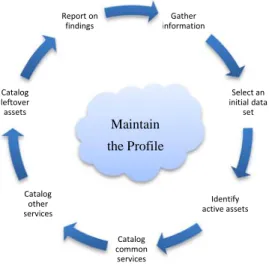
The general steps for network profiling as detailed in this report are as follows: (1) gather available network information, (2) select an initial data set, (3) identify the active address space, (4) catalog common services, (5) catalog other services, (6) catalog leftover assets, and (7) report on findings. These steps can be turned into a cyclic feedback loop to maintain the profile as shown in Figure 1.

Figure 1: Network Profiling Process Cycle

Before beginning, ensure there are enough resources to devote to this exercise. This process should be completed within a fixed amount of time so that the results are relevant. For networks with relatively fixed assets, this process could take place over one to two months. For faster changing networks, it could take place in as little as one to two weeks. The amount of time and

Gather information Select an initial data set Identify active assets Catalog common services Catalog other services Catalog leftover assets Report on findings Maintain the Profile

(14)

other resources that it will take to complete the process depends primarily on the size of the network and how well the assets conform to networking common practices.

Throughout this report, validation will be discussed as a key component of the profiling process. It is essential to validate results before adding them to the profile. In general, there are two types of validation: active and passive. Passive validation uses only stored data without extra resources. Active validation involves using manual effort to validate initial findings by attempting to make connections to the specific IP address and using third-party references. For example, one can validate a potential web server by browsing to port 80 or by performing a name server lookup on that IP address. When manual validation is not possible through these means, communication with the owner or administrator of the device may be necessary, if possible.

This process uses netflow traffic to perform an analysis. We used the System for Internet-Level Knowledge (SiLK)1 tool to collect and analyze the traffic, and we include examples of the SilK commands and results of the commands in each of the steps. However, the steps apply to any flow analysis tool.

1.1 Sample Data

We demonstrate how to create a network profile using sample data collected from the perimeter of an enterprise network. These data were anonymized after analysis to protect the confidentiality of the network owner without impairing the data’s usefulness.

1.2 The SiLK Analysis Tool Suite

Because the case study in this report uses SiLK for analysis, you should understand how SiLK records flow data.

SiLK deals with uniflow traffic, meaning traffic coming into the network is recorded as separate flows from traffic going out of the network. Although SiLK differentiates between inbound and outbound traffic based on the source and destination IP addresses, it does not attempt to identify traffic as either client or server, as do some other flow platforms.

SiLK is configured by setting an address range for the internal network. The type of flow is then based on whether the source and destination IP addresses are inside or outside of that range. As shown in Figure 2, a flow of type “in” is defined as traffic with an external source address and internal destination address. A flow of type “out” is defined as traffic with an internal source address and an external destination address.

Figure 2: SiLK Flow Types

1

For more information, visit http://tools.netsa.cert.org/silk/. Out

Internal range

(15)

Web traffic is separated from all other traffic and is defined in SiLK by default as traffic to or from ports 80, 443, or 8080 and is labeled as “inweb” or “outweb” based on the same reasoning as flows of type “in” or “out.”

1.3 Keeping Track of Findings

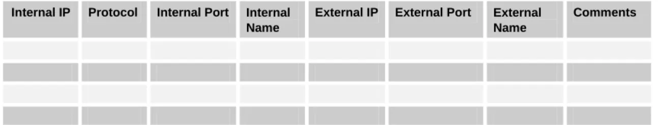
A spreadsheet like Table 1 is extremely useful to record findings throughout the profiling process. The headers you choose will depend on the information that is needed about the network and may be adapted for each step of the process.

Table 1: Example Profiling Spreadsheet

Internal IP Protocol Internal Port Internal

Name

External IP External Port External

Name

Comments

Throughout the process, record the commands and tools used to gather and validate the data. This record will enable automation of certain parts of the process, making future updates less labor intensive, and will allow for reproducible results. As an example, shell scripts have been included in Appendix B of this report. Note that the scripts are provided only for reference and may or may not be appropriate for a specific network.

1.4 Extending the Analysis

The steps in this report are, by no means, the only way to use network flow data to learn about a network. As you get comfortable using the features of the analysis tool, you should feel capable of delving into further detail if the traffic flows look interesting or out of place. Flow data can be used for forensics purposes, for finding malicious activity, and for determining appropriate packet prioritization settings, among other things.

(16)

2 Gather Available Network Information

Gathering any available information about the network prior to beginning the profile is an important step because it will help set the scope for the rest of the process. The types of information that could be collected include items such as address space, network maps, lists of servers and proxies, and policies governing network design. This information may be incomplete or out of date, but it provides, at a minimum, a starting point for known devices and a reference for potential problem points that may arise during the profiling process that require additional effort to validate. Familiarity with the organization’s network and security policies is also beneficial, as it enables the profiler to notice discrepancies between the policies and the actual findings. The output of the profiling effort may reveal compliance issues or may suggest potential changes to security policies that are worth considering.

It is important to know what you expect to see when starting the profile, but it is just as important to realize that not everything about the network is known. For example, an old File Transfer Protocol (FTP) server dedicated to internal file sharing may have been temporarily opened to outside services but then forgotten about when that capability was no longer needed. Such carelessness can lead to lack of information, which results in holes in network security. If time allows, consider conducting a quick assessment or penetration test to develop a network map and a list of exposed services on various machines. Many automated tools, some free such as nmap,2 are available for network mapping, and most network monitoring solutions have built-in network mapping capabilities. Be sure to obtain permission to run active scans on a network before doing so, as initiating active scans and probes could violate company policy or negatively affect the performance of systems and services on the network.

When the profile is complete, update the network maps and lists of servers so that the process can be cycled through again in the future.

2.1 Sample Network Information

For the purposes of this report’s case study, we initially assumed only the following about the network being profiled:

• size: thousands of users

• owner: a mid-sized organization using the network for its business purposes

• CIDR: 203.0.113.0/24 (203.0.113.0 – 203.0.113.255)

2

“Nmap (‘Network Mapper’) is a free and open source (license) utility for network exploration or security auditing.” Source: nmap.org

(17)

3 Select an Initial Data Set

Choosing the initial data set for analysis is important because it shapes the entire analysis. Take some time to obtain a good representative sample of data that still remains a reasonable size. A data set large enough to represent typical traffic is necessary, but it should be small enough to be able to iteratively process queries.

Before selecting the initial data set, understand how the sensor placement and flow collection configurations affect the available flow data.

3.1 Sensor Placement and Configuration

The importance of sensor placement should not be underestimated. Placement affects what flow data is and is not collected, as well as which IP addresses are associated with each flow record. The following framework will help you decide the most effective sensor placement and

configuration for the network you will profile.

Proper sensor placement for network profiling takes into account several considerations: the goal of the flow collection—in this case, network profiling—the network topology, and the network hardware in use. For example, some network hardware or network security devices, such as proxy servers or firewalls, can make visibility into the network difficult or impossible with flow data alone. The goal of this report’s step-by-step process is to profile perimeter traffic to see what a network looks like when viewed externally by a potential attacker. Therefore, sensors should be placed on the external, or internet-facing, side of any perimeter networking devices. Sensor placement for other goals may have different requirements and is, thus, out of the scope of this report.

When a network is split up into intranets, it is tempting to profile each one individually. Remember, the goal is to profile the network from the view of an outsider, so place the sensors around the perimeter of the largest extranet that needs to be profiled. If necessary, divide the data collected by address blocks to view differences between intranets. Note that profiling anything except the entire network may leave out assets not intended to be left out.

Remote and business-to-business networks often have their own gateway into a network. Include these gateways when placing sensors at all access points to the network. Note any special access points like these so that you are aware that traffic across these sensors may be different than typical traffic at other sensors. This same reasoning applies to business continuity links, which should be included in the profile with a note that traffic at these sensors will be different than traffic at other sensors. Table 2 contains guidelines for sensor placement.

Table 2: Sensor Placement Guidelines

Configuration Placement

Multiple exit points Make sure all access points connecting the network to other networks are covered.

Network/security devices (proxies, NATs, firewalls, etc.)

(18)

Configuration Placement

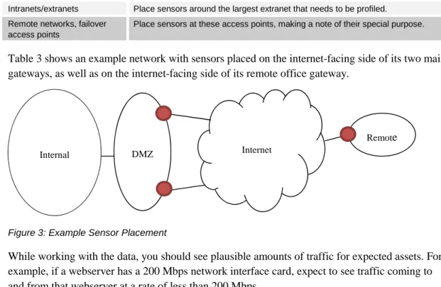
Intranets/extranets Place sensors around the largest extranet that needs to be profiled. Remote networks, failover

access points

Place sensors at these access points, making a note of their special purpose.

Table 3 shows an example network with sensors placed on the internet-facing side of its two main gateways, as well as on the internet-facing side of its remote office gateway.

Figure 3: Example Sensor Placement

While working with the data, you should see plausible amounts of traffic for expected assets. For example, if a webserver has a 200 Mbps network interface card, expect to see traffic coming to and from that webserver at a rate of less than 200 Mbps.

3.2 Guidelines

Guidelines for selecting a sample data set are listed in Table 3. It is not necessary to ensure that the sample data set is representative of all traffic that crosses the network boundary. Once built, the profile will be reapplied to the rest of the data set to make sure nothing is missed. Selecting a sample data set should be done after the sensors are placed and network flow has been collected.

Table 3: Guidelines for Selecting a Data Set

Feature Considerations

Duration Start with at least an hour’s worth of data. Add more data—up to a day’s worth—until the query time starts to slow down. The query time for the entire initial data set should be 15-60 seconds.

Timing Select the busiest time of day to quickly carve out the most common network traffic.

Direction If the traffic is bidirectional and it is necessary to further reduce the sample size in order to reduce the query time, start by looking at outbound traffic—traffic that is generated by internal equipment. Sampling Avoid starting with sampled data if possible because it may mask some important and routine

behaviors. Network

size

If the network is extremely large but divides into logical boundaries by IP address, consider separating the analysis into a few independent profiles and merging them after you complete the analysis. For the sample network, we used the following command to choose a day’s worth of data from Wednesday, September 28, 2011, which is representative of a typical workday, as the sample data set.

$ rwfilter --start-date=2011/09/28:00 --end-date=2011/09/28:23 \ --type=all --protocol=0- --pass=sample.rw

Internet

Remote

(19)

Note: rwfilter is the main SiLK command, which allows selection and partitioning of flow records based on various fields in the record.

In the case of the sample network, there was enough processing power to query a data set of this size. No other filtering was done based on start or end times, flow duration, address space, direction, or other characteristics.

The following example shows the command we performed on the sample data set and the result that it has 10,985,967 total records and is 571 MB in size.

$ rwfileinfo sample.rw sample.rw: format(id) FT_RWGENERIC(0x16) version 16 byte-order littleEndian compression(id) none(0) header-length 156 record-length 52 record-version 5 silk-version 2.4.2 count-records 10985967 file-size 571270440 command-lines

1 rwfilter --type=all --start-date=2011/09/28:00 \ --end-date=2011/09/28:23 --protocol=0- --pass=sample.rw

3.3 Validating the Selection

After identifying a sample data set to work with, it is worthwhile to take a few extra minutes to do some surface analysis of the sample to confirm that it seems to represent the network. A quick inspection of the sample will save time that could otherwise be wasted on an improperly collected or filtered data set.

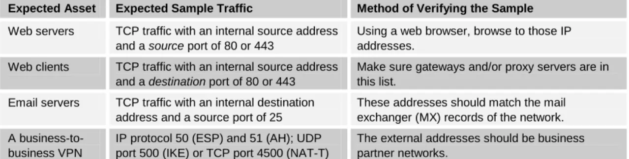
The highest volume data paths should be no surprise and should be obvious in the data set. Check typical ports, protocols, and address blocks to ensure the sample contains expected data. Table 4 includes a few possible tests for validating the selection.

Table 4: Validating the Initial Data Set

Expected Asset Expected Sample Traffic Method of Verifying the Sample

Web servers TCP traffic with an internal source address and a source port of 80 or 443

Using a web browser, browse to those IP addresses.

Web clients TCP traffic with an internal source address and a destination port of 80 or 443

Make sure gateways and/or proxy servers are in this list.

Email servers TCP traffic with an internal destination address and a source port of 25

These addresses should match the mail exchanger (MX) records of the network. A

business-to-business VPN

IP protocol 50 (ESP) and 51 (AH); UDP port 500 (IKE) or TCP port 4500 (NAT-T)

The external addresses should be business partner networks.

(20)

3.3.1 Sample Network Data Set Validation

Because there was no network map or list of servers for the sample network, the sample data set was validated by inspecting for the types of traffic typically seen during a workday on a business network. Basic networking knowledge indicates that almost all of the traffic should be over TCP and UDP. This can be verified by dividing the traffic volumes for the sample network based on IP protocol number and looking at the top five protocols in use. The following command and output from the sample data show that there was also some ICMP (protocol 1) traffic, and ESP and IPv4 encapsulation protocols (50 and 4 respectively).

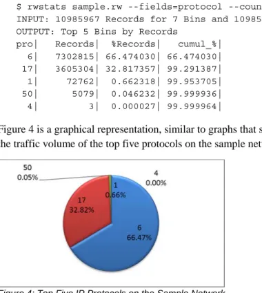
$ rwstats sample.rw --fields=protocol --count=5

INPUT: 10985967 Records for 7 Bins and 10985967 Total Records OUTPUT: Top 5 Bins by Records

pro| Records| %Records| cumul_%| 6| 7302815| 66.474030| 66.474030| 17| 3605304| 32.817357| 99.291387| 1| 72762| 0.662318| 99.953705| 50| 5079| 0.046232| 99.999936| 4| 3| 0.000027| 99.999964|

Figure 4 is a graphical representation, similar to graphs that some network analysis tools create, of the traffic volume of the top five protocols on the sample network.

Figure 4: Top Five IP Protocols on the Sample Network

Note: In SiLK, rwstats is the command that groups flows by a specific key or, in this case, protocol, and prints the top values by traffic volume percentage. Other analysis tools may show this graphically, as seen in Figure 4.

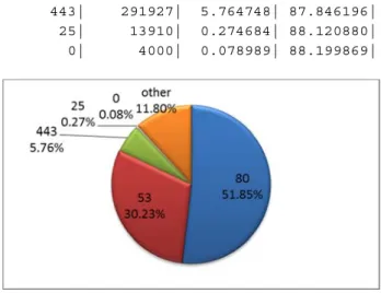
The top expected services requested by clients on a typical network are web (ports 80 and 443), DNS (53), and SMTP (25), so verify by sorting outgoing traffic into the top five most common destination ports. The statistics that follow the SiLK command below and are represented graphically in Figure 5 show some traffic to port zero, which is SiLK’s notation for traffic on IP protocols other than TCP and UDP.

$ rwfilter sample.rw --type=out,outweb --protocol=0- --pass=stdout \ | rwstats --count=5 --fields=dport

dPort| Records| %Records| cumul_%| 80| 2625707| 51.850423| 51.850423| 53| 1530900| 30.231025| 82.081448|

(21)

443| 291927| 5.764748| 87.846196| 25| 13910| 0.274684| 88.120880| 0| 4000| 0.078989| 88.199869|

Figure 5: Destination Ports for Outbound Traffic from the Sample Network

The output shows that the expected services are being used. Also, servers on the network are likely to handle the same services.

Next, check the source port of outbound traffic. The SiLK command and the output from the sample network follow.

$ rwfilter sample.rw --type=out,outweb --protocol=0- --pass=stdout \ | rwstats --count=5 --fields=sport

sPort| Records| %Records| cumul_%| 53| 291693| 5.760127| 5.760127| 80| 129093| 2.549228| 8.309355| 25| 85331| 1.685050| 9.994406| 443| 71429| 1.410524| 11.404930| 0| 6644| 0.131201| 11.536131|

Figure 6 shows the top five source ports in relation to the rest of the outbound traffic (labeled “other” in the graphic).

Figure 6: Source Ports for Outbound Traffic from the Sample Network

This second analysis shows that the services in use—DNS, web, and email servers—are as expected. You can safely assume at this point that the available data has been properly sampled and can proceed with the profiling process.

(22)

4 Identify the Monitored Address Space

Start network profiling activities by becoming familiar with the network address topology and how well the sensors can see it. Some issues involving monitored address space are whether sensors cover any private address space, what traffic is expected on failover circuits during normal operations, and whether a business unit has connected a system without administrator knowledge. This section explores some of these issues by first finding populated addresses. The process to identify the monitored address space follows these steps:

1. Identify hosts that have active TCP connections.

2. Identify hosts that generate a nontrivial amount of traffic on protocols other than TCP. 3. Aggregate individual hosts into populated network blocks.

4. Examine additional information to confirm the list of active IP address blocks.

Figure 7 shows steps 1 and 2. Upon completing all four steps, you will have an idea of the active hosts that are seen by the network sensors. The intent at this point is not to identify and name every observed device, but simply to understand sensor coverage and compare it with what is already known about the topology of the network.

Figure 7: Active Hosts 4.1 TCP Talkers

For most networks, the bulk of traffic happens on TCP (IP protocol 6). Therefore, you can find most active network hosts (also referred to as “talkers”) by looking for legitimate TCP sessions. Sustained TCP conversations are relatively easy to identify in flow. However, pay careful attention to eliminate scan traffic and “ghost” traffic—attempts to connect to hosts that no longer exist. The purpose of getting rid of the ghost traffic is not because it is inconsequential, but simply because it is not helpful for identifying active internal hosts. Criteria for finding active TCP hosts are listed in Table 5.

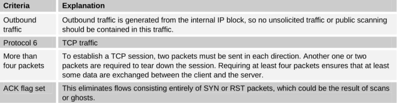
Table 5: Active TCP Host Criteria

Criteria Explanation

Outbound traffic

Outbound traffic is generated from the internal IP block, so no unsolicited traffic or public scanning should be contained in this traffic.

Protocol 6 TCP traffic More than

four packets

To establish a TCP session, two packets must be sent in each direction. Another one or two packets are required to tear down the session. Requiring at least four packets ensures that at least some data are exchanged between the client and the server.

ACK flag set This eliminates flows consisting entirely of SYN or RST packets, which could be the result of scans or ghosts.

Step 2

Step 1 TCP

UDP Other

(23)

Use the following command to apply these filter criteria to the sample traffic and obtain a list of the source IP addresses actively using TCP.

$ rwfilter sample.rw --type=out,outweb \ --protocol=6 --packets=4- --ack-flag=1 --pass=stdout \ | rwset --sip-file=tcp_talkers.set

$ rwsetcat tcp_talkers.set --count 36

The command’s output shows that the sample network has 36 active TCP talkers. The addresses of these hosts were placed into a SiLK set file3 for future reference. Saving the list of IP addresses is an important step to eliminate redundant queries later on.

4.2 Other Talkers

TCP was used to identify active hosts first to eliminate as much scanning and ghost activity as possible; however, many connectionless protocols are used on networks. In addition to finding TCP talkers, it is important to find IP addresses on the network that are actively using other protocols.

You should separate web-browsing traffic (ports 80, 8080, and 443) from all other traffic if the analysis software has the capability to do so. Web-browsing traffic is not normally carried over protocols other than TCP. Leave out this traffic over non-TCP protocols for now.4 See the following commands as an example.

$ rwfilter sample.rw --type=out --protocol=0-5,7-255 --pass=stdout \ | rwset --sip-file=other_talkers.set

$ rwsetcat --count other_talkers.set 25

The output of these commands shows that the sample network has 25 active talkers on other protocols.

4.3 Aggregating Hosts

You should now have two lists of active addresses—TCP and non-TCP. Join the lists together and remove any duplicates. The result will be all of the active assets from the sample set, without too much extraneous traffic. If the list is large, consider dividing it into groups of smaller netblocks for separate analysis. The SiLK command for joining the TCP and non-TCP lists follows.

$ rwsettool --union tcp_talkers.set other_talkers.set \ --output-path=talkers.set

$ rwsetcat --count talkers.set 40

Combining the TCP and “other talkers” lists for the sample network results in 40 active talkers, as shown in the command output above.

3

The SiLK set file is located at http://tools.netsa.cert.org/silk/rwset.html.

4

In SiLK, “out” traffic does not include traffic to or from ports 80, 8080, or 443; those are included in “outweb” traffic.

(24)

If this number seems small given the size of the netblock being analyzed, remember that the sensors have been placed on the external side of perimeter networking devices. It is very likely that client traffic is going through proxies or Network Address Translation (NAT) servers prior to reaching the sensor.

It may be helpful for larger networks to aggregate the IP addresses into netblocks.5 The following example includes the command and output.

$ rwsetcat talkers.set --network-structure=X 203.0.113.0/27| 9 203.0.113.32/27| 8 203.0.113.64/27| 5 203.0.113.96/27| 1 203.0.113.160/27| 4 203.0.113.192/27| 13

If necessary, you can profile the addresses in each block separately.

Once you complete these steps, you will no longer need the TCP talkers and other talkers lists. 4.4 Supplemental Analysis and Validation

Some network monitoring systems may have visualization capabilities that chart the most active hosts or services, plot port usage across time,6 or view a graph of IP addresses versus ports. If these tools are available, use them to get an overview of the traffic and hosts on the network, but be careful about relying on them for profiling. In general, visualizations are not detailed enough to get an accurate picture of what is going on in a network, but they can help guide the process. Once the process is complete, visualizations become important for reporting and reference material.

Use graphs to supplement the analysis, but do not rely on them as a final authority. Use the information gathered previously about the network to validate the active hosts. For example, if there are supposed to be 10 servers in the demilitarized zone (DMZ) but the active hosts list has only five entries, there may be either a misconfiguration on the network or a misplaced sensor.

4.5 Anomalies

You should now have a list of active hosts on the network, as seen by the outside world; however, in rare cases, some of this traffic may be merely passing through (transiting) the network. Check for transit traffic by looking for traffic leaving the network that is not from an internal host. Conversely, it may also be worthwhile to check for any traffic heading into the network from an internal host (if inbound traffic is available) and for any traffic heading out of the network to an internal host. The following example shows the command and results of this step.

5

Choose from –-network-structure=[A,B,C,X] to define /8, /16, /24, or /27 address blocks, respectively.

6

(25)

$ rwfilter sample.rw --type=out,outweb --not-sipset=talkers.set \ --print-statistics

Files 1. Read 10985967. Pass 0. Fail 10985967. $ rwfilter sample.rw --type=in,inweb --sipset=talkers.set \ --print-statistics

Files 1. Read 10985967. Pass 0. Fail 10985967. $ rwfilter sample.rw --type=out,outweb --dipset=talkers.set \ --print-statistics

Files 1. Read 10985967. Pass 0. Fail 10985967. In the sample network, no transit traffic was found. In fact, the collection system is configured with the correct netblock of internal IP addresses and set to record internal-to-internal

communication separately from other communication. Understand how the specific collection system for the network being profiled is configured before moving on with this process. Asymmetric routing can also create difficulties for interpreting flow traffic and may occur in networks with two or more active internet connections. If sensors do not cover the alternate connections, traffic may not be collected from one direction of the flow. Different flow tools handle asymmetric routing in different ways, so it is important to be aware of how the netflow analysis tool you’re using handles asymmetric routing and to adjust the procedure accordingly. For example, with the SiLK flow analysis suite, unique flows are determined based on protocol, source IP, source port, destination IP, and destination port. SiLK creates a separate flow for each direction of an actual flow. Therefore, the choice of using outbound traffic only for finding active talkers was appropriate because asymmetric routing was not a factor.

(26)

5 Catalog

Common

Services

After identifying the active hosts on the network, continue the profile by inventorying the services that typically constitute the majority of bandwidth usage and business operations, such as web traffic (both client and server) and email. Once you have carved these protocols out of the data set, start working on other services that are likely to be on the network and also visible to instrumentation: Virtual Private Network (VPN), Domain Name Server (DNS), and FTP, and other less used but common protocols. This section includes a template for cataloging other services that may not specifically be listed but make up a large part of the traffic volume on the network.

5.1 Web Servers

Web servers are often the easiest asset to profile and will commonly constitute a large percentage of web traffic. Start by looking for connections into the network destined to a service running on ports 80, 8080, or 443. Also consider whether any other web services are running on the network that would require adding a port to this list, such as streaming services or a port configuration different from the default. For example, web services sometimes reside on ports 81 or 82.

5.1.1 The Process

1. Compile a list of the busiest IP addresses with connections coming from ports 80, 8080, and 443. Filter out flows that do not complete a TCP handshake (the SYN, SYN-ACK, ACK traffic pattern used to initiate TCP connections) by selecting only flows that have an ACK flag set and that are at least four packets long. This will eliminate scans and accidental attempts to connect. Choose only addresses that make up at least 1% of the traffic being profiled (in bytes). These are the busiest web servers. The SiLK command and output from the sample data for this process follow.

$ rwfilter sample.rw --type=outweb \ --sport=80,443,8080 --protocol=6 --packets=4- --ack-flag=1 \ --pass=stdout \ | rwstats --fields=sip --percentage=1 --bytes

INPUT: 190814 Records for 24 Bins and 15207959195 Total Bytes OUTPUT: Top 7 bins by Bytes (1% == 152079591)

sIP| Bytes| %Bytes| cumul_%| 203.0.113.69| 7888143831| 51.868523| 51.868523| 203.0.113.28| 3272828647| 21.520499| 73.389022| 203.0.113.198| 2631884565| 17.305968| 90.694990| 203.0.113.194| 652195072| 4.288511| 94.983501| 203.0.113.196| 255865129| 1.682442| 96.665944| 203.0.113.44| 254700968| 1.674787| 98.340731| 203.0.113.197| 152764557| 1.004504| 99.345235|

The result of the above command is a list of seven IP addresses accounting for 99.34% of the web server traffic. Save this list of IP addresses as a file named web_servers, as in the following example. It will be needed several times during the profiling process.

(27)

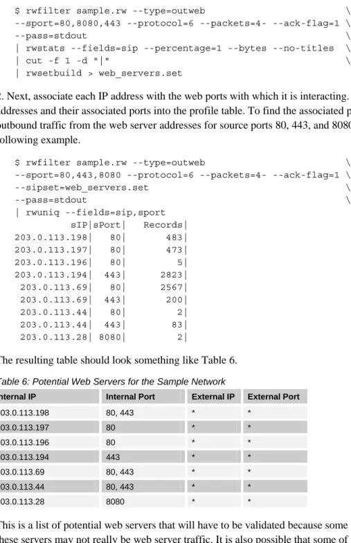
$ rwfilter sample.rw --type=outweb \ --sport=80,8080,443 --protocol=6 --packets=4- --ack-flag=1 \ --pass=stdout \ | rwstats --fields=sip --percentage=1 --bytes --no-titles \ | cut -f 1 -d "|" \ | rwsetbuild > web_servers.set

2. Next, associate each IP address with the web ports with which it is interacting. Place these addresses and their associated ports into the profile table. To find the associated ports, filter outbound traffic from the web server addresses for source ports 80, 443, and 8080, as in the following example.

$ rwfilter sample.rw --type=outweb \ --sport=80,443,8080 --protocol=6 --packets=4- --ack-flag=1 \ --sipset=web_servers.set \ --pass=stdout \ | rwuniq --fields=sip,sport sIP|sPort| Records| 203.0.113.198| 80| 483| 203.0.113.197| 80| 473| 203.0.113.196| 80| 5| 203.0.113.194| 443| 2823| 203.0.113.69| 80| 2567| 203.0.113.69| 443| 200| 203.0.113.44| 80| 2| 203.0.113.44| 443| 83| 203.0.113.28| 8080| 2|

The resulting table should look something like Table 6.

Table 6: Potential Web Servers for the Sample Network

Internal IP Internal Port External IP External Port

203.0.113.198 80, 443 * * 203.0.113.197 80 * * 203.0.113.196 80 * * 203.0.113.194 443 * * 203.0.113.69 80, 443 * * 203.0.113.44 80, 443 * * 203.0.113.28 8080 * *

This is a list of potential web servers that will have to be validated because some of the traffic to these servers may not really be web server traffic. It is also possible that some of the actual web servers on the network have not been detected in this step but will be detected in other steps in the profiling process. It is important to keep the profile table updated.

5.1.2 How to Validate Findings

Web servers should be easy to validate using a web browser. Manually go to each site, checking the address with both HTTP and HTTPS to verify that the associated ports in the table are correct. If possible, do this from outside the network, as the server may be configured to accept different types of traffic from the internal network, which could conflict with earlier findings. A

(28)

nonresponsive server could mean that the server is offline, it has been configured not to accept connections from certain networks, or it has been taken over for malicious purposes. Consider documenting a brief description of the services running on the server for future reference. Resolve each IP address to a domain name using nslookup (reverse and forward) or some other tool and ensure that the result matches what is expected on the network. If it does, add the domain name as a field in the profile table. If it does not match, it may be an old server that no one realized was still running on the network, or it may be an anomaly. The reverse record may not match if the machine is in a shared hosting environment.

Check the server certificate of the servers associated with port 443. The common name on the certificate should match the server’s domain name. If it does not match, there could be a security concern. Also, confirm that the certificate has not expired; this is a common cause of errors received by clients accessing sites over HTTPS that have not been properly maintained. If it is still unclear which of these addresses are actually web servers, try looking at the external addresses connecting to them. If there are only a few, it could be a web server locked down to a few addresses, or possibly a point-to-point SSL VPN; but if there are many external sources, it probably is an actual web server. Examine the number of distinct external addresses, their address blocks, and the timing of requests to get a feel for whether the traffic is actual HTTP traffic. Some flow analysis tools attempt to label traffic based on content characteristics. This can be very helpful when trying to identify traffic that is not obvious based on header information.

Several of the IP addresses from the sample network listed as potential web servers were validated by using nslookup and by browsing to their addresses. Even though there is no traffic to port 443 on several of the servers, on others the port is open and presents an expired certificate. Also, some of the sites are using mirrors, such that multiple IP addresses are actually assigned to the same website. This is common for servers that receive heavy traffic.

One of the servers on the same network could not be validated using the above simple methods, so we took a closer look at the inbound TCP traffic to that address. Address 203.0.113.28 served only one IP address during the sample time frame as seen in the following example.

$ rwfilter sample.rw --type=outweb --sport=80,443,8080 --packets=4- \ --protocol=6 --ack-flag=1 --saddress=203.0.113.28 --pass=stdout \ | rwuniq --fields=dip

dIP| Records| 198.51.100.12| 1|

In the example below, the records that resulted from the command show that the traffic from this external IP is composed of one very long flow. The flow is divided into half-hour chunks because that is how SiLK collects flows.

$ rwfilter sample.rw --type=outweb \ --sport=80,8080,443 --protocol=6 --packets=4- --ack-flag=1 \ --saddress=203.0.113.28 \ --pass=stdout \ | rwcut --fields=stime,etime,bytes,flags

sTime| eTime| bytes| flags| 2011/09/28T00:15:32.577|2011/09/28T00:45:32.568| 68169846| PA | 2011/09/28T00:45:32.634|2011/09/28T01:15:32.567| 68272876| PA |

(29)

2011/09/28T01:15:32.609|2011/09/28T01:45:32.605| 68270589| PA | 2011/09/28T01:45:32.643|2011/09/28T02:15:32.640| 68252975| PA | 2011/09/28T02:15:32.646|2011/09/28T02:45:32.635| 68334416| PA | 2011/09/28T02:45:32.658|2011/09/28T03:15:32.653| 68310047| PA | ...| ...| ...| ...| 2011/09/28T23:45:33.247|2011/09/29T00:15:33.218| 68245623| PA | This is not typical traffic to a web server, so we deleted this IP address from the table of web servers. We show how to profile it in a later section.

5.1.3 Anomalies

The following is a list of anomalies that should be considered when determining which IP addresses are web servers.

• client traffic

Servers normally do not have legitimate client traffic. Expected traffic would be from software updates or an administrator troubleshooting a problem on the server. If there is a web server with a lot of client traffic, it is probably some type of gateway and should go into a different category.

• streaming media services

Some servers are meant for serving streaming media to clients. These servers have open ports that are different from the HTTP and HTTPS ports. Check for traffic coming into the network using UPD and TCP ports such as 1935, 1755, and 554.

• SSL VPNs

Long-duration, high-volume connections on port 443 could be SSL VPN connections. More discussion is in Section 5.5 on VPNs.

• one server that sits on many IP addresses

This situation should become clear upon resolving the IP addresses to DNS names. This is not a security issue, but it should be noted in the profile table.

• many websites that sit on one IP address

This should also become clear when many IP addresses resolve to the same DNS name with a forward lookup (not necessarily a reverse lookup). Again, note this in the profile table.

• business continuity and server failover

If the network has backup servers that are either turned off or are handling only small amounts of traffic until they are needed, the servers probably will not be observed in this section. Use the information gathered at the beginning of this exercise to list these servers in the profile table and note that they are backup servers.

• spurious RSTs

Web servers often send reset packets to close a connection instead of waiting for the standard TCP FIN-ACK. This action is harmless and does not have an effect on profiling the asset.

• mobile devices and embedded web servers

With today’s technology, a surprising number of devices have web servers embedded in them; common devices include VOIP phones, mobile devices, print servers, and copiers.

(30)

5.1.4 Results

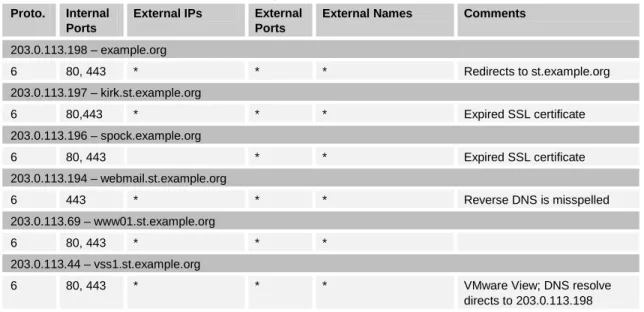
Sample network results from the validated web servers are in Table 7.

Table 7: Validated Web Servers for the Sample Network

Proto. Internal

Ports

External IPs External

Ports

External Names Comments

203.0.113.198 – example.org 6 80, 443 * * * Redirects to st.example.org 203.0.113.197 – kirk.st.example.org 6 80,443 * * * Expired SSL certificate 203.0.113.196 – spock.example.org 6 80, 443 * * Expired SSL certificate 203.0.113.194 – webmail.st.example.org 6 443 * * * Reverse DNS is misspelled 203.0.113.69 – www01.st.example.org 6 80, 443 * * * 203.0.113.44 – vss1.st.example.org

6 80, 443 * * * VMware View; DNS resolve

(31)

5.2 Client Web

Client web traffic is usually the most common traffic on any network. For the purposes of this report, client web traffic will include HTTP, HTTPS, Shockwave, and other streaming media. It is important to separate web traffic from services like SSH, VPN, and file sharing because these services are managed very differently than web traffic.

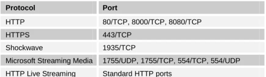
The ports listed in Table 8 are the most common ports for web client traffic. You will find any additional web client protocols when you analyze leftover ports.

Table 8: Services for Normal Client Web Traffic

The process for finding web clients is similar but opposite to the process for finding web servers. Instead of looking for traffic coming from web ports on the internal host, look for traffic going to web ports on an external host, as shown in Figure 8.

Figure 8: Process for Finding Web Clients

1. Start by filtering for legitimate TCP traffic on the ports in Table 8, as shown in the following command. The traffic should be outbound to the ports on IP protocol 6 (TCP) with at least four packets per flow and the ACK flag set.

$ rwfilter sample.rw --type=out,outweb \ --protocol=6 --ack-flag=1 --packets=4- \ --dport=80,8000,8080,443,1935,1755,554 \ --pass=stdout \ | rwset --sip-file=tcp_clients.set

2. Add in the UDP traffic to the ports in Table 8 using the following command. $ rwfilter sample.rw --type=out,outweb \

--protocol=17 --dport=1755,554 \ --pass=stdout \ | rwset --sip-file=udp_clients.set

3. Listing legitimate TCP-only (flows of four packets or more with an ACK flag) and UDP flows separately ignores some scanning traffic. Looking at outbound rather than inbound traffic also

Protocol Port

HTTP 80/TCP, 8000/TCP, 8080/TCP

HTTPS 443/TCP

Shockwave 1935/TCP

Microsoft Streaming Media 1755/UDP, 1755/TCP, 554/TCP, 554/UDP HTTP Live Streaming Standard HTTP ports

Port 80 External Web Server Port 80 External Web Client

(32)

helps with this. After both lists are created, combine them for analysis, as in the following example.

$ rwsettool --union tcp_clients.set udp_clients.set \ --output-path=web_clients.set

$ rwsetcat --count web_clients.set 31

The output from the above command shows that the sample network has 31 web clients. Look at only the hosts with at least 1% of the client web traffic on the network because most hosts will act as web clients at some point. Even DNS, web, and other servers often have some web traffic from updates or configuration changes; but this traffic is usually minimal. When using a proxy, there should be very few internal IPs that fall into this category because the client traffic will be funneled through these devices. If this is not the case, it may be useful to try profiling the workstations separately from other hosts (separate them based on traffic volume).

4. The bulk of the packets for client web traffic will be inbound. Therefore, filter incoming traffic if possible.

$ rwfilter sample.rw --type=in,inweb \ --dipset=web_clients.set --sport=80,8080,8000,443,1935,1755,554 \ --pass=stdout \ | rwstats --fields=dip --bytes --percentage=1

INPUT: 2973484 Records for 31 Bins and 168273056846 Total Bytes OUTPUT: Top 2 bins by Bytes (1% == 1682730568)

dIP| Bytes| %Bytes| cumul_%| 203.0.113.33| 154723380928| 91.947804| 91.947804| 203.0.113.220| 12334655077| 7.330143| 99.277947|

The above command results in a list of two IP addresses accounting for 99.27% of the client web traffic. Update the profile to include only the results from filtering incoming traffic.

5. If it is not possible to filter inbound traffic, use the following filter on outbound traffic. This filter checks traffic going from the web clients to external web servers, rather than traffic coming from external web servers to the internal web clients as the previous filter does.

$ rwfilter sample.rw --type=out,outweb \ --sipset=web_clients.set --dport=80,8080,8000,443,1935,1755,554 \ --pass=stdout \ | rwstats --fields=sip --percentage=1

INPUT: 2921867 Records for 32 Bins and 2921867 Total Records OUTPUT: Top 2 bins by Records (1% == 29218)

sIP| Records| %Records| cumul_%| 203.0.113.33| 2625228| 89.847621| 89.847621| 203.0.113.220| 274448| 9.392898| 99.240520|

6. Next, associate each IP address with the ports and protocols with which it is interacting using the command in the following example, which also shows the output. Place these addresses and their associated ports into the profile table.

(33)

$ rwfilter sample.rw --type=out,outweb \ --sipset=web_clients.set --dport=80,8000,8080,443,1935,1755,554 \ --pass=stdout \ | rwuniq --fields=sip,dport,protocol sIP|dPort|pro| Records| 203.0.113.220| 80| 6| 235334| 203.0.113.220| 443| 6| 38733| 203.0.113.220| 554| 6| 5| 203.0.113.220| 8080| 6| 95| 203.0.113.220| 1935| 6| 281| 203.0.113.33| 1935| 6| 128| 203.0.113.33| 443| 6| 251473| 203.0.113.33| 8000| 6| 1| 203.0.113.33| 8080| 6| 895| 203.0.113.33| 80| 6| 2372731|

The sample network has web clients as shown in Table 9, which were added to the full profile.

Table 9: Potential Web Clients for the Sample Network

Internal IP Internal

Port

External IP

External Port Protocol

203.0.113.220 * * 80, 443, 554, 1935, 8080 6 203.0.113.33 * * 80, 443, 1935, 8000, 8080 6 Follow the next section to carefully validate this list of potential web clients. 5.2.2 How to Validate Findings

Web clients are more difficult to validate than web servers. Look for three types of web clients: proxy servers, NAT gateways, and directly connected workstations that do not use a proxy or NAT server. This requires looking at inbound traffic as well as outbound. Some of the addresses in the list might not be web clients at all.

The different types of web clients can be determined based on several characteristics. The first are traffic volume and timing. Directly connected workstations typically have traffic patterns that match the schedule of the organization. As with the sample network, many organizations have no after-hours or weekend traffic, and their daily traffic volume tends to be very small. Web

gateways (NAT servers) have a high volume of traffic. Web proxy servers have a medium to high volume of traffic.

For the sample network, the traffic volume for the web clients is as follows.

$ rwfilter sample.rw --type=out,outweb \ --sipset=web_clients.set --dport=80,8080,8000,443,1935,1755,554 \ --pass=stdout \ | rwstats --fields=sip --bytes --count=2

INPUT: 3029615 Records for 15228 Bins and 168278493869 Total Bytes OUTPUT: Top 2 Bins by Bytes

sIP| Bytes| %Bytes| cumul_%| 203.0.113.33| 154723380928| 91.944833| 91.944833| 203.0.113.220| 12334655077| 7.329906| 99.274739|

(34)

Based on traffic volume alone, one can make an educated guess that the top IP address (203.0.113.33) is a web gateway and the other is a web proxy server.

Another characteristic to check is whether the client is running any other services. Client

workstations usually do not have any services running. Web gateways are likely to look as if they host services because they are often gateways for the rest of the services on the network. A client that looks as if it is hosting many services could also be a VPN gateway. Web proxies are not as likely to host other services unless they come with services configured by default.

To keep the list size manageable, look for common services such DNS, FTP, SSH, SMTP, HTTP, and HTTPS. The following output shows the command and results for looking for common services.

$ rwfilter sample.rw --type=out,outweb \ --sipset=web_clients.set --sport=20,21,22,25,53,80,8000,8080,443 \ --pass=stdout \ | rwuniq --fields=sip,sport sIP|sPort| Records| 203.0.113.220| 8080| 7| 203.0.113.220| 8000| 7| 203.0.113.33| 20| 1| 203.0.113.33| 443| 492| 203.0.113.33| 21| 27| 203.0.113.33| 8000| 44| 203.0.113.33| 8080| 58| 203.0.113.33| 22| 7| 203.0.113.33| 80| 42|

Because 203.0.113.33 makes connections over so many ports, as the example’s output shows, there is a good chance that it is actually a multipurpose gateway or a VPN gateway. We removed it from the web clients list and show how to profile it later in this report.

There may be a fair amount of high port traffic, indicating that clients are using various host-based applications or streaming media. Also, most client operating systems use ephemeral ports in a sequential fashion within a certain range. For example, if most clients on the network are Windows 7 machines that use the range 49152 to 65535, look for hosts using ports starting on the lower end to make connections and working their way up to port 65535.

If plotting software is available, it may help to view ephemeral port usage over time. This will allow you to quickly see sequential port usage and what range is being used. This is a method often referred to as “passive fingerprinting.”

After we checked traffic volume, services, and port usage of the potential web clients on the sample network, we validated the one client left on the list as an actual web proxy server. 5.2.3 Anomalies

Almost all machines at some point generate a small amount of web traffic, whether they are servers, gateways, or local hosts. Client web traffic coming from machines that serve another purpose can be ignored because it does not need to be part of the profile. If this traffic is of

(35)

concern for security reasons, look into the flows in more detail, or check firewall/proxy logs and configurations.

Here is a more detailed description of some of the anomalies mentioned in Section 5.2.2 about validation.

• directly connected workstations hosting services

Client operating systems come with certain services preinstalled. Sometimes those services are left on by default. So, just because services are hosted at an address does not necessarily indicate that the machine is a server or gateway. Look at the specific service being hosted and the amount of traffic connecting to it.

• servers with client web traffic

Though servers sometimes use web traffic to get their updates or configuration changes, this traffic is usually minimal and received from a small number of external addresses. If this is the only client web traffic to an address in the list, that address probably should not be listed as a web client.

• other types of traffic over web ports

Just because there is traffic at the typical web ports does not mean it is HTTP or streaming traffic. Any service can be configured to use those ports. This is often done for application ease of use or to get around firewall policies.

5.2.4 Results

The sample network had one web client that was added to the profile as listed in Table 10.

Table 10: Final Web Clients for the Sample Network

Proto. Internal Port External IP External Port External Name Comments

203.0.113.220

(36)

5.3 Email

Email services are provided through several different protocols. The most common protocol for sending mail across the internet is Simple Mail Transfer Protocol (SMTP) on TCP port 25. SMTP traffic is mostly server-to-server traffic. Email clients, desktop clients in particular, do not use SMTP but instead submit emails to the SMTP server at port 587 to be forwarded by the server. To receive messages, clients use Post Office Protocol (POP), Internet Message Access Protocol (IMAP), or web mail.

Email protocols allow for encryption over the standard TCP ports outlined above. However, some additional ports are set aside for encrypted email sessions. These are less commonly used but may still show up on networks. Email ports are listed in Table 11.

Table 11: Email Ports and Protocols

1. Using the following command, start by looking for email servers, which will send traffic from the SMTP, POP3, and IMAP ports listed in Table 11. Look for outgoing traffic with a source TCP equal to those ports and an IP protocol of 6. TCP port 587 (MSA) is not used here because it is only used with inbound traffic to servers.

$ rwfilter sample.rw --type=out \ --protocol=6 --ack-flag=1 --packets=4- --sport=25,465,110,995,143,993 \ --pass=stdout \ | rwset --sip-file=smtp_servers.set

The results of the above command on the sample network are listed in Table 12.

Table 12: Potential Email Servers for the Sample Network

Internal IP Internal Port External IP External Port

203.0.113.231 25 * *

203.0.113.195 25 * *

203.0.113.221 25 * *

203.0.113.220 25 * *

203.0.113.222 25 * *

Because the sensors for the sample network are located on the internet-facing side of the network, no IMAP or POP traffic is seen between internal clients and servers. Only server SMTP traffic is seen by the sensor.

2. Now look for potential email clients. Depending on where the sensors are placed, client traffic may not cross the flow collectors because it only has to go as far as the mail server on the

Protocol Port Encrypted Session Port

SMTP 25 465

POP3 110 995

IMAP 143 993

(37)

network. This a good test to see if any clients are sending email directly outside of the network without using standard mail services.

3. Desktop email clients typically submit messages to TCP port 587 and collect them from TCP ports 110 and 143 (or encrypted ports 995 and 993), so filter outbound traffic for these ports using the following command.

$ rwfilter sample.rw --type=out \ --protocol=6 --packets=4- --ack-flag=1 --dport=110,143,587,995,993 \ --pass=stdout \ | rwset --sip-file=email_clients.set

The sample network did not have any email clients visible in the day-long sample data set, a strong indicator that its internal hosts are correctly set up to get their (corporate) email through the network’s email servers. It could also mean that hosts are getting all their email through web mail. 5.3.2 How to Validate Findings

Once again, it is important to validate the results for the email servers and clients. Potential servers sending mail out of the network to TCP port 25 are almost guaranteed to be servers. This can be thought of as an email server’s way of acting as client to other servers on the internet. Filtering for this traffic on the sample network validates two addresses. The following example shows the command results.

$ rwfilter sample.rw --type=out \ --protocol=6 --packets=4- --ack-flag=1 --dport=25,465 \ --pass=stdout \ | rwuniq --fields=sip

sIP| Records| 203.0.113.222| 10479| 203.0.113.231| 74852|

Servers can also be validated using nslookup for each of the addresses in the list or using the MX record of the domain. Obtain the MX record by typing the following command:

nslookup –type=MX example.org

The result should be a list of servers, like the one below, that relay email to and from the domain. Non-authoritative answer:

example.org mail exchanger = 10 checkov.example.org. example.org mail exchanger = 20 sulu.example.org.

Use this list of mail exchanger servers as a guide to help with validation. Using a regular DNS lookup on each address in the server list can help you validate simply by looking at the name of the server (all externally facing SMTP servers will have a DNS record and associated IP address). Telnetting to each IP address at port 25 may also produce a banner message hinting at the purpose of a machine. These messages sometimes contain error information that is specific to a particular operating system or service running on the remote machine.

As a result of using these methods, all but one of the addresses was verified as an email server— 203.0.113.220, which was listed in the previous section as a gateway for web client traffic. It

(38)

looks as if this address may also be proxying email traffic, which indicates that it is probably a main gateway for all client traffic.

Email servers almost always come with a default web mail application. This means that these email servers are also basically acting as web servers. Unfortunately, these web servers are not usually discovered when filtering for web servers (as done in Section 5.1) because of their low traffic volume. After the email servers have been validated, test each one for a running web mail application by going to each server’s address in a web browser. Try this on both ports 80 and 443. As is often the case, the sample network was running web applications on two of its email servers. Both were open to connections over HTTP, meaning email login credentials were being sent in plain text.

It is slightly more difficult to validate client email traffic because there is not usually any external information to use in the validation. Try searching the web for a particular client address to see if it shows up in any email headers. Also, try looking at the traffic in more detail to see if it matches expected client traffic.

5.3.3 Anomalies

Email service is probably the most straightforward service discussed in this report. However, there are some anomalies to be aware of.

• nondedicated email servers

Email servers do not necessarily have to be dedicated machines. They can, and often do, run in parallel with other services, especially web services. So, it is acceptable if an IP address of an email server has already been listed as a web server because it is just one machine running several different services.

• clients acting as servers

Because email services do not have to be on dedicated servers, any host can run an email server, even a client. If an IP address in a client subnet is listed as a server or an IP address is listed as both a server and a client, this is probably what is happening. These servers will likely have a very low SMTP traffic volume compared to the other servers. Check policies on clients hosting such services and firewall configurations. (On most networks, only certain IPs should be allowed to send and receive SMTP traffic.)

• desktop clients sending SMTP messages

It is possible for client machines to be configured to send their messages to port 25 (SMTP) rather than port 587 (MSA). Investigate any clients that bypass the internal email

(39)

5.3.4 Results

The sample network has four SMTP mail servers and no externally facing mail clients, as listed in Table 13.

Table 13: Validated Email Assets for the Sample Network

Proto. Internal

Port

External IP External

Port

External Name Comments

203.0.113.231 - smtpfw.st.example.org 6 25 * * 6 * * 25 203.0.113.195 - sulu.example.org 6 25 * * 6 * * 25 203.0.113.221 - omail.example.org 6 25 * * 6 * * 25

6 80 * * Plain-text email login

203.0.113.222 – imail.example.org

6 25 * *

6 * * 25

(40)

5.4 Domain Name System

The Domain Name System (DNS) provides multiple services [Mockapetris 1987]. The most common is the translation between domain names and IP addresses. A network will likely contain both DNS clients and DNS servers. The standard port for DNS is 53, usually carried over UDP. Transactions may also take place over TCP when larger amounts of data need to be transferred, such as when zone transfers occur. However, zone transfers rarely take place across perimeter boundaries. On a network, the servers will be the hosts accepting connections on port 53, and the clients will be those communicating with services on port 53.

Servers support either recursive or iterative query resolution. Recursive servers take the responsibility of looking up the complete answer for the client, recurring, if necessary, from the root (“.”) to the top-level domain (“.com”) to the second-level domain (“example.com”) and so forth, and only then responding to the client’s request. Recursive servers will typically

communicate with numerous other servers across the internet. Iterative servers, on the other hand, accept requests but do not do recursive resolution. If an iterative server has the information necessary to answer the request, it gives that information to the client. Otherwise, it responds with an error or a referral to another DNS server. The client is then responsible for querying the next DNS server. This means that you should never see iterative servers issuing DNS requests.

1. Begin the DNS inventory with a summary of the DNS traffic on the network. Look for the top DNS (port 53) traffic inbound and outbound and the top external addresses receiving the

network’s DNS traffic. Sort traffic volumes by the number of packets rather than the number of bytes or flows because almost every DNS request or response is contained in a single UDP packet.

The top 10 external DNS servers that were queried by the sample network using the following command are shown in the output below. Their IP addresses have been converted to domain names using SiLK’s built-in resolver function.

$ rwfilter sample.rw --type=out \ --dport=53 --protocol=17 \ --pass=stdout \ | rwstats --count=10 --fields=dip --packets \ | rwresolve

INPUT: 1530863 Records for 12559 Bins and 1629508 Total Packets OUTPUT: Top 10 Bins by Packets

dIP| Packets| %Packets| cumul_%| dns.publicprovider.com| 533435| 32.735955| 32.735955| 192.0.2.1| 173289| 10.634437| 43.370392| provider.net| 113603| 6.971614| 50.342005| d.gtld-servers.net| 19974| 1.225769| 51.567774| a.gtld-servers.net| 18015| 1.105548| 52.673322| c.gtld-servers.net| 16703| 1.025033| 53.698356| l.gtld-servers.net| 16620| 1.019940| 54.718295| b.gtld-servers.net| 15752| 0.966672| 55.684967| f.gtld-servers.net| 15657| 0.960842| 56.645810| g.gtld-servers.net| 15378| 0.943720| 57.589530|