Spectral Methods for Semi-supervised Manifold Learning

Spectral Methods for Semi-supervised Manifold Learning

Zhenyue Zhang

Department of Mathematics, Zhejiang University

Hangzhou 310027, China

[email protected]

Hongyuan Zha and Min Zhang

College of Computing, Georgia Tech

Atlanta, GA 30332

Abstract

Given a finite number of data points sampled from a low-dimensional manifold embedded in a high dimensional space together with the parameter vectors for a subset of the data points, we need to determine the parameter vec-tors for the rest of the data points. This problem is known as semi-supervised manifold learning, and in this paper we propose methods to handle this problem by solving certain eigenvalue-problems. Our proposed methods address two key issues in semi-supervised manifold learning: 1) fitting of the local affine geometric structures, and 2) preserving the global manifold structures embodied in the overlapping neighborhoods around each data points. We augment the alignment matrix of local tangent space alignment (LTSA) with the orthogonal projection based on the known parame-ter vectors, giving rise to the eigenvalue problem that char-acterizes the semi-supervised manifold learning problem. We also discuss the roles of different types of neighborhoods and their influence on the learning process. We illustrate the performance of the proposed methods using both synthetic data sets as well as data sets arising from applications in video annotations.

1. Introduction

Many problems in pattern recognition and computer vi-sion generate high-dimenvi-sional data whose variations can be characterized by a small number of parameters. Mani-fold learning is a popular unsupervised learning approach aiming at recovering the low-dimensional parameterization from a finite set of high-dimensional data points sampled from the manifold [6,7]. Several manifold learning algo-rithms have been proposed and applied to problems in pat-tern recognition and computer vision. One important issue, however, has largely been ignored, at least not explicitly ad-dressed in the past: the fact that there exist infinitely many nonlinear parameterizations for the same manifold. If the parameterization is isometric, it makes sense to aim at re-covering the isometric parameterization (up to a rigid

mo-tion). In the more general case, the problem seems to be ill-defined, which parameterization out of the infinitely many possible ones to aim at? We argue that in applications one is interested in thesemantically meaningful parameteriza-tions,1_{and extra information is needed to tell those} param-eterizations from the rest. One type of extra information is in the form of labeled data: a subset of the data points are labeled with the corresponding semantically meaningful pa-rameter vectors, and we need to compute the semantically meaningful parameter vectors for the rest of the data points. This type of semi-supervised manifold learning problems are the focus of this paper. Some variations of the prob-lems have been discussed before [3,8], but we want to em-phasize the crucial role it plays in recovering semantically meaningful and physically relevant parameterizations. We now proceed to a more formal discussion of the problems.

2. Semi-supervised manifold learning

LetMbe a parameterizedd-dimensional manifold em-bedded inRD with D d, i.e., there is a one-to-one function φ defined on a sub-domain Ω of Rd such that

M=φ(Ω)[4]. We callφa parameterization ofM. Obvi-ously, the parameterization ofMis not unique; for any one-to-one transformationψfrom a sub-domainΔtoΩ,φ◦ψ

is another parameterization ofM. Generally, we need to determine some parameterizationφwhich is semantically meaningful to the application we are considering.

Given data pointsx₁, . . . , x_N sampled from the mani-fold M, we want to compute the corresponding seman-tically meaningful parameter vectors which we designate asy₁, . . . , yN. Generally, the yi’s may even live in Rn

withn = d. To deal with this generality, we assume that

y₁, . . . , yN are sampled from another parameterized

mani-foldMsembedded inRn_{, and bothMandMsshare the}

samed-dimensional parameter spaceΩ. So there are two functionsφandψdefined on the same domainΩsuch that

M=φ(Ω), Ms=ψ(Ω). (1)

1_{The video annotation problem discussed in section is a very good}

il-lustrative example.

Furthermore,xi = φ(τi), yi = ψ(τi), i = 1, . . . , N. We

see

y=ψ(τ) =ψ(φ−1(x)) =ψ◦φ−1(x) =g(x),

andyi = g(xi). Now we can state the problem of

semi-supervised manifold learning as follows.

Without loss of generalities, we assumex1,· · ·, xare

labelled with parameter vectorsy₁,· · ·, y, we want to

de-termine the parameter vectorsyiforxi, i=+ 1, . . . , N,

or more importantly, we also want to estimate the function

g:M → Msas accurately as possible from the data.

3. Local tangent space alignment (LTSA)

Our proposed semi-supervised manifold learning meth-ods can be considered as an adaptation of LTSA to the semi-supervised setting. For this reason, we first give a brief re-view of LTSA [9]. Along the way we also introduce the concepts oftangent coordinatesand thealignment matrix

which are key ingredients of our proposed algorithms. For a given set of sample pointsx₁, . . . , xN, we begin

with building a connectivity graph on top of them which specifies, for each sample point, which subset of the sam-ple points constitutes its neighborhood [6]. Let the set of neighbors for the sample pointx_ibeX_i= [x_i1, . . . , x_iki], includingxiitself. We approximate those neighbors using

ad-dimensional (affine) linear space,

xij ≈x¯i+Qiθ(ji), Qi= [q1(i), . . . , qd(i)], j= 1, . . . , ki,

wherex¯i is the mean of thexij’s, d is the dimension of

the manifold,Qi is an orthonormal basis matrix. Theθj(i)

are the localtangent coordinatesassociated with the basis matrix, i.e.,θ_j(i) =QT

i(xj−x¯i). Using the singular value

decomposition of the centered matrixXi−x¯ieT,Qican be

computed as the left singular vectors corresponding to thed

largest singular values ofXi−x¯ieT [2].

We postulate that in each neighborhood, the correspond-ing global parameter vectorsTi= [τi1, . . . , τi_ki]differ from

the local onesΘi = [θ1(i), . . . , θk(ii)]by a local affine

trans-formation. The errors of the optimal affine transformation is then given by min ci,Li ki j=1 τij−(ci+Liθ(ji))22 = min ci,Li Ti−(cieT+LiΘi)2F =TiΦi2F, (2)

whereΦiis the orthogonal projection whose null space is

spanned by the columns of[e,ΘT

i]. We seek to compute the

parameter vectorsτ1, . . . , τN by minimizing the following

objective function, N i TiΦi2F = trace(TΦTT) (3) overT = [τ1, . . . , τN]. Here Φ = N i=1 S_iΦ_iST i (4)

is thealignment matrixwithSi∈RN×ki, the 0-1selection matrix, such thatTi = T Si. Imposing certain

normaliza-tion condinormaliza-tions onT such asTTT =IdandT e= 0,2the

corresponding optimization problem

min{trace(TΦTT_{)|T T}T _=I

d, T e= 0,}

is solved by computing the eigenvectors corresponding to the2nd tod+ 1st smallest eigenvaluesλ₂,· · ·, λd+1ofΦ, here the eigenvalues ofΦare arranged in nondecreasing or-der, i.e.,λ₁ = 0 ≤ λ₂ ≤ · · · ≤ λd+1 ≤ · · · ≤ λN.The

firstd+ 1 smallest eigenvalues are quite small generally, compared with others. We mention that if the parameteri-zationφis isometric, then under certain conditions, LTSA can recover the isometric parameterization.

4. Local structures of parameterizations

A manifold can admit many different parameterizations. However, each parameterization locally can be approxi-mately characterized by the tangent coordinates discussed above. This property motivates us to consider a spectral solution for the semi-supervised problem: find a global pa-rameter system that minimizes this kind of local approxima-tion errors (on all labelled and unlabelled points) as well as the least squares approximation errors on labels. In this sec-tion, we first give a detailed analysis for the local structures of parameterizations.

Consider a parameterizationφ: Ω→ Mof the manifold

MwithΩ ⊂ Rd_{. LetT}

ˆ

x be the tangent space ofMat

ˆ

x=φ(ˆτ). Consider a small neighborhoodΩ(ˆτ)ofˆτsuch that the orthogonal projection ofφ(τ)ontoTx_ˆis one-to-one.

Letθbe the tangent coordinate ofφ(τ)corresponding to an orthogonal basisQxˆofTˆx, i.e.,

θ=QT_xˆ(φ(τ)−φ(ˆτ)), τ∈Ω(ˆτ). (5) Consider the Taylor expansion of first order ofφat pointτˆ,

φ(τ) = φ(ˆτ) +Jτˆ(τ−τˆ) +(τ,τˆ). (6) HereJ_ˆτis the gradient matrix ofφatτˆand(τ,τˆ)the sec-ond order term ofτ−τˆ,

(τ,τˆ) = 1

2JτTˆHτˆ(τ−τ , τˆ −τˆ) +o(τ−τˆ2)

with the Hessian tensorHˆτofφatτˆ, respectively. It follows

from (6) that

τ−τˆ = (J_τˆTJτˆ)−1JτˆT

φ(τ)−φ(ˆτ)

+(J_τˆTJτˆ)−1(τ,τˆ). (7)

Note that Jτˆ = QτˆPτˆ with nonsingular matrix Pτˆ = QT

ˆ

τJτˆ. Substituting it into (7) and using (5), we obtain that τ−τˆ=P_τˆ−1θ+ (P_τˆTPτˆ)−1(τ,τˆ).

Equivalently,

τ= ˆτ+P_τˆ−1θ+ (P_τˆTP_ˆτ)−1(τ,ˆτ). (8)

The equality (8) shows the affine relation between the local tangent coordinatesθ ofx, which can be estimated from a neighbor set ofx, and the global coordinatesτ. Note that the affine transformationˆτ+P_ˆτ−1θis also local. The ”affine” difference between the two coordinates is of second order ofτ−τˆ,

τ−(ˆτ+P_τˆ−1θ) ≤σmin(Jτˆ)−2(τ,τˆ)

≤ JτTˆHˆτ

2σ_min2 (Jτˆ)

τ−τˆ2+o(τ−ˆτ2). (9)

Hereσmin(·) denotes the smallest singular value of a ma-trix and we have usedPT

ˆ

τ Pτˆ = JˆτTJˆτ. Furthermore, the

error bound above is o(τ −ˆτ2) for isometric φ since

JT

τ Hτ(u, v) = 0for anyτ,u, andv.

The semantically meaningful parameter vectory of a manifoldMgenerally will have dimension different from the intrinsic dimension ofM. Referring to (1), by the Tay-lor expansion ofψ,

ψ(τ) =ψ(ˆτ) +J_τˆψ(τ−ˆτ) +ψ(τ,τˆ),

and using (8), we see that

y= ˆy+J_τˆψP_τˆ−1θ+J_τˆψ(P_τˆTP_ˆτ)−1(τ,τˆ) +ψ(τ,ˆτ).

Therefore, we also have the following estimation for a gen-eral parameterization, y−(ˆy+L_τˆθ)c_φ,ψ(ˆτ)τ−ˆτ2 (10) with cφ,ψ(ˆτ) = 1 2 J_τˆψJT ˆ τHˆτ σ_min2 (Jˆτ) +(J_τψ_ˆ)TH_τψ_ˆ . (11)

We summarize the above discussion in the following the-orem.

Theorem 1 Assume thatφ: Ω→ Mis a smooth function.

Ω(ˆτ)is a neighborhood ofτˆ∈Ωandρ(Ω(ˆτ))denotes its diameter. Lety=ψ(τ)∈ Rmis a user interested parame-ter variable of the manifold. Ifφis not rank-deficient atτˆ, i.e. σ_min(J_ˆτ)= 0, then the coordinateyis affine equal to its tangent coordinateθwith errorO(ρ2(Ω(ˆτ)))inΩ(ˆτ). Furthermore, if bothφ and ψ are isometric, the error is o(ρ2(Ω(ˆτ))).

5. Spectral methods

Theorem1shows that the local structures of the desired parameterizationy=g(x)withg=ψ◦φ−1can be recov-ered by an affine transformation of the local tangent coordi-nates. Denote byziestimatesofyi=g(xi),i= 1,· · ·, N.

Letxi1,· · · , xi_kibe a set of neighbors ofxiwith the

corre-spondingyi1, . . . , yi_ki ∈Ω(yi), a neighborhood ofyi. The

affine transformationyˆ_i+L−_τˆi1θin (10) can be estimated as

(c+Lθ) = arg min c,L ki j=1 zij−(c+Lθ( i) j )2,

hereθ_j(i)are the local tangent coordinates. Then by (10)

1 ki trace(ZiΦiZiT) = 1 ki ki j=1 zij−(c+Lθ (i) j )2 ≈ c2_φ,ψ(τi)ρ4(Ω(τi)) +o(ρ4(Ω(τi))).

HereZi = [zi1,· · ·, ziki], andΦi is the orthogonal

pro-jection whose null space is span([e,ΘT

i]) with Θi =

[θ₁(i),· · · , θ_k(i_i)]. Summing over all the data points, and let

Φbe the alignment matrix in (4),

1 Ntrace(ZΦZ T_{) =} 1 N N i=1 1 ki ki j=1 zij−(c+Lθ( i) j )2 ≤max i c2_φ,ψ(τi)ρ4(Ω(τi)) +o(max i ρ 4_(Ω(τ i))) .

The above analysis shows that ifghas bounded gradient and Hessian, the parameter vectorsyi give rise to small

trace(ZΦZT_{). We emphasize that Φ embodies two}

re-quirements: 1) local affine equivalence to the tangent coor-dinates as illustrated above; and 2) smooth global manifold structure through the overlaps among the neighborhoods.

Besides a small trace(ZΦZT), the estimate Z should also satisfy the constraints that it should be close to the known parameter vectors. Without loss of generality, we assume thatYL = [y1,· · ·, y], N are known. Then ZL = [z1,· · ·, z] should be close to YL. This can be

achieved by minimizing the difference betweenZland an

affine transformation ofYL, min c,L 1 i=1 zi−(c−Lyi)2 = 1 trace(ZLPYLZ T L) = 1 trace(ZSLPYLS T LZT),

wherePYLis the orthogonal projection whose null space is

span([e, Y_LT]).

We now combine the two types of constraints to arrive at following optimization problem,

min ZZT=I Ze=0 1 Ntrace(ZΦZ T_{) +}λ trace(ZSLPYLSTLZT), (12)

which amounts to computing the 2nd to (d+1)-st smallest eigenvectors u2,· · ·, u+1 of the symmetric and positive

semi-definite matrix

Ψ = Φ +βSLPYLSLT (13)

withβ = λN , since eis a trivial eigenvector ofΨ corre-sponding to the zero eigenvalue.

Affine Transformation.The constraintZZT _=I dis a

convenient one to use in (12), but the resultingZneeds an affine transformationz → c+W z in order to match the known parameter vectors. There are several possible ways to do this. We present a simple one as follows. We compute

(c+W z) = arg min c,W p j=1 yj−(c+W zj)22. (14)

Its solution is[c, W]QT₁₁ = Y1,where Q11is the subma-trix of rows inU₁ = [u₁,· · · , u+1]corresponding to the labeled set. In terms of numerical stability, the labeled set should be selected such thatQ₁₁ has as small a condition number as possible. This is the main idea of AE selection given in [8]. Note that hereQ₁₁also depends on the selec-tion of the labelled set. So it is hard to select the prior points in the ”optimal” way. In general, ifQ11is close to singular, one may regularize the linear system using a smallη > 0

and obtain the regularized solution,

[c, W] =Y1Q11(QT₁₁Q11+ηQ112I)−1.

Oncec and W are computed, the{zi} are then affinely transformed to ˜zi = c+W zi, i = + 1,· · ·, N with Z2= [z+1,· · ·, zN].

6. Some improvements

We now present some improvements over the approach outlined in the above section by taking a closer look at the different roles played by the various data points in their con-tribution to the alignment matrixΦ. To this end, we split

Φinto three parts: 1) neighborhoods of labeled points, 2) neighborhoods containing at least a labeled points, and 3) other neighborhoods, Φ = j=1 SjΦjSjT+ p i=+1 SiΦiSiT+ N i=p+1 SiΦiSiT,

where we assume that the neighborhood of eachxi,i = + 1,· · · , p, contains at least one labeled point and other neighbor sets ofxi, i > p, have no labeled points in their

neighbors. We will modifyΦby introducing two tuning parametersα= [α₁, α₂]with1> α₁, α₂>0, Φ(α) =α1 j=1 SjΦjSjT+ p i=+1 SiΦiSiT+α2 N i=p+1 SiΦiSiT. 0 2 4 0 1 2 3 4 5

Figure 1. The incomplete tire manifold with samples (left) and generating coordinates of the samples (right).

The basic idea is thatxi, i = + 1,· · ·, pare the

neigh-borhoods that connect the labeled data points with the un-labeled data points, and should be assigned larger weights. Then the eigen-problem (12) becomes

min ZZT=I,Ze=0ZΨ(α, β)Z T_{, (15)} whereΨ(α, β) = Φ(α) +βS_LP ST Lwithβ= λN.

7. Numerical experiments

We present several numerical expamples to illustrate our proposed algorithms and compare them with the least squares (LS) method [8] and the Laplacian regression method (LapRLS) [1]. The data selection method is the one used in [8] which is briefly discussed at the end of section 5. Two data sets are considered: one is a toy data set from a non-isometric 2D manifold embedded in 3D space. The other is a video sequence and we are interested in annota-tions of the frames in the video sequence.

Example 1.Consider a section of a torus with a middle slice removed and its parameterization given by

g(s, t) = ⎡

⎣ (3 + cos(3 + cosss) cos) sintt

sins ⎤

⎦, (s, t)∈[0,5π

3 ]2.

It is a 2D manifold embedded inR3and is not isometric (d= 2, D= 3). We sampleN = 500pointsxj=g(sj, tj)

from the manifold with the generating parameter vectors

(sj, tj)uniformly distributed in the domain[0,5₃π]2. Figure

6shows the manifold, the sample points and their generat-ing parameters.

We labeled = 50of the data points with their corre-sponding 2D generating parameter coordinates, and applied the proposed spectral method with8neighbors of eachxi

(includingxi itself) to recover the parameters(s, t), and α1 = 2α, α2 = α with a range of values of α and λ. The spectral approach works well and is not sensitive to the choice of the turning parametersαandβ. In Tables1we list the value of102(α, β), where(α, β) is the relative Frobenius norm of the total errors of unlabeled pointsZU L,

with respect to differentα’s and β’s. We set d = 2 for construct the alignment matrixΦ(α). We point out that the optimal parametersαandβdepend on the selection of the prior points when the number of labelled points is fixed.

Table 1.102(α, β)of the eigen-system approach with LM

selec-tion. α\β 10−1 100 101 102 103 104 0.01 2.12 1.56 1.47 1.46 1.46 1.46 0.02 2.17 1.49 1.39 1.38 1.38 1.38 0.03 2.32 1.49 1.38 1.37 1.37 1.37 0.04 2.52 1.53 1.40 1.39 1.38 1.38 0.05 2.72 1.59 1.44 1.42 1.42 1.42

We also compared our spectral method with the LS method in [8] and LapRLS in [1]. A range of parameters were used with ’rbf’ kernel and ’heat’ weights for Lapla-cian graph, including the neighborhood sizekof each point

xi(not includingxiitself) listed as follows, KernelP aram ∈ [10−3, 103], GraphW eightP aram ∈ [10−4, 103], γ_A ∈ [10−4, 103], γI ∈ [10−3, 103].

The smallest result is achieved with error0.0715atk= 10, kernel parameter1.5, graph weight parameter1000,γA =

0.0005, andγI = 0.004. Generally, LapRLS is quite

sen-sitive to the choice of the parameters. The smallest er-ror is much larger than the erer-ror0.01365by our spectral method using same labelling. The error of the LS method

is0.03363. Figure 2 plots the computed generating

coor-dinates by the three methods: the spectral method, the LS method and LapRLS.

0 2 4 0 1 2 3 4 5 Spectral Method: ε = 0.0137 0 2 4 0 1 2 3 4 5 LS Method: ε = 0.0336 0 2 4 0 1 2 3 4 5 LapRLS:ε = 0.0715

Figure 2. The computed coordinates (red circles) by our spectral method (left), the LS method (middle), and LapRLS (right), to-gether with the generating coordinates (blue dots) of the incom-plete tire.

Example 2. This is video sequence consisting of 393 frames of a subject sitting in a sofa and waving his arms.3

3_{From http://www.csail.mit.edu/ rahimi/manif. The original data set}

has984frames. We deleted identical frames from the data set.

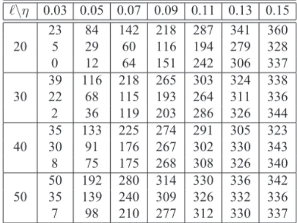
Table 2. Numbers of correct position vectors ofunlabeledpoints

computed by spectral method (top rows), LS method (middle row), and LapRLS (bottom rows) within given accuracy.

\η 0.03 0.05 0.07 0.09 0.11 0.13 0.15 23 84 142 218 287 341 360 20 5 29 60 116 194 279 328 0 12 64 151 242 306 337 39 116 218 265 303 324 338 30 22 68 115 193 264 311 336 2 36 119 203 286 326 344 35 133 225 274 291 305 323 40 30 91 176 267 302 330 343 8 75 175 268 308 326 340 50 192 280 314 330 336 342 50 35 139 240 309 326 332 336 7 98 210 277 312 330 337

We are interested in annotating the frames with the posi-tions of the subject’s arms that are determined by the four points of the elbows and wrists in the frames. Soy_iare now

8-dimensional vectors containing the four 2D points. The relative error function of a computed vectorziis defined as (zi) =||zi−yi||/a, i=+ 1, ..., N, (16)

whereais the diameter of image rectangle.

In table2, we list the number of the computed position vectors of the unlabeled points satisfying a given accuracy threshold η, i.e., (zi) < η. The turning parameters of

the spectral method are simply set asα₁ = α₂ = 1and

β = 200for all. We search the parameter space for the

’rnf’ kernel parameter,γAandγIin the interval[10−3,103]

and choose the following: ’rbf’ kernel parameter100, heat weight parameter 10−3, andγA = 10−3, γI = 10−3,

which give the best results. Figure3 plots the computed arm positions (blue bars) by the spectral method (= 50) against the manually labeled positions (red dots) on several illustrative examples with increasing amount of error.

Our spectral method performs better than the LS method and LapRLS. First, it has higher accuracy on the unlabeled images as shown in Table2. Second, our method is not as sensitive to the turning parameters. For example, the spec-tral method gives almost the same results for(α1, α2, β)∈

[1, 100]×[1, 100]×[50, 500]if= 50. We remark that the factorγ˜I = NγI2 of the term used in the Laplacian ma-trix in (35) of [1] is very small,γ˜I = 6.4746×10−9for

the optimalγI. It seems that the Laplacian does not play

a positive role for this real data set. If we increase˜γI to

10−4_{with the others unchanged, the smallest position} er-ror min₃₀(zi) of unlabeld points computed by LapRLS

is 0.085. Figure 4 plots the error cures for the spectral method, LS method, and LapRLS method ( = 30) with

γI

param-# 51

# 89

#127

#165

#203

#241

#279

#317

#355

#393

Figure 3. Computed arm-positions (blue bars) by the spectral method (= 50) and labelled points (red dots) in increasing order of errors.

0 50 100 150 200 250 300 350 0 05 .1 5 .2 25 Spectral LS LapRLS,γI/N 2_=1.e−6 LapRLS,γI/N 2_=1.e−5 LapRLS,γI/N 2_=5.e−5 LapRLS,γI/N 2_=1.e−4

Figure 4. The error curves of the spectral method, LS method, and

LapRLS method with γI

N2 = 10−6,10−5,₂110−4,10−4,= 30.

eters remain unchanged.

8. Conclusion

We proposed methods for semi-supervised manifold learning by solving eigenvalue problems. We emphasize the important role played by semi-supervised manifold learn-ing in computlearn-ing semantically meanlearn-ingful parameteriza-tions of manifolds embedded in high-dimensional spaces. Several topics need further investigation: 1) developing ac-tive learning methods to select the data points to label for the proposed spectral methods; and 2) explore other prob-lem structures such as the dynamics of the scene in video annotations for semi-supervised manifold learning.

Acknowledgments. The work was supported in part by NSFC grant 10771194 and NSF grant DMS-0736328.

References

[1] M. Belkin, P. Niyogi and V. Sindhwani. Manifold reg-ularization: a geometric framework for learning from Labeled and Unlabeled Examples.Journal of Machine Learning Research, 6: 2399–2424, 2006.4,5 [2] G. H. Golub and C. F Van Loan. Matrix

Compu-tations. Johns Hopkins University Press, Baltimore, Maryland, 3nd edition, 1996.2

[3] J. Ham, I. Ahn and D. Lee. Learning a manifold-constrained map between image sets: applications to matching and pose estimation.CVPR, 2006.1 [4] J. Munkres. Analysis on Manifold Addison Wesley,

Redwood City, CA, 1990.1

[5] A. Rahimi, B. Recht and T. Darrell. Learning appear-ance manifolds from video. CVPR, 2005.

[6] S. Roweis and L. Saul. Nonlinear dimensionality re-duction by locally linear embedding. Science, 290: 2323–2326, 2000.1,2

[7] J. Tenenbaum, V. De Silva and J. Langford. A global geometric framework for nonlinear dimension reduc-tion. Science, 290:2319–2323, 2000.1

[8] X. Yang, H. Fu, H. Zha and J. Barlow. Semi-supervised nonlinear dimensionality reduction.ICML, 2006.1,4,5

[9] Z. Zhang and H. Zha. Principal manifolds and nonlin-ear dimensionality reduction via tangent space align-ment. SIAM J. Scientific Computing. 26:313-338, 2005.2