Novel methods in transcriptome analysis using RNA-seq

(1)

c

(2)

NOVEL METHODS IN TRANSCRIPTOME ANALYSIS

USING RNA-SEQ

BY

YANG LI

THESIS

Submitted in partial fulfillment of the requirements

for the degree of Master of Science in Bioengineering

in the Graduate College of the

University of Illinois at Urbana-Champaign, 2012

Urbana, Illinois

Adviser:

(3)

Abstract

RNA-seq has proven to be a powerful technique for transcriptome profiling based on next-generation sequencing (NGS) technologies. Using RNA-seq, we want to solve two critical challenges: identifying Splice Junctions (SJs) and annotating gene fusion transcripts.

Due to the limited read length of NGS data, it is extremely challenging to accurately map RNA-seq reads to SJs, which is important for the analysis of alternative splicing and isoform construction. In this thesis, we describe a novel method, called TrueSight, that combines information from (i) RNA-seq read mapping quality and (ii) coding potential from the reference genome sequences into a unified model that utilizes semi-supervised self-training to precisely identify SJs. Both simulation and real data evaluations showed that TrueSight achieved higher sensitivity and specificity than existing tools.

We also applied TrueSight to discover novel splice forms in honey bee transcriptomes that cannot be detected by other methods and found that 94.6% of honey bee multi-exon genes are alternatively spliced. Utilizing high coverage transcriptome profiling data and a gene model enhanced by TrueSight, our quantitative analysis revealed that the expression ratio of the splice variants from a single gene is significantly correlated with the gene’s exon-intron structure, splice site strength, and methylation pattern. We believe this new tool will be highly useful to comprehensively study splice variants based on RNA-seq.

Fusion transcripts can be created as a result of genome rearrangement in cancer. Some of them play important roles in carcinogenesis, and can serve as diagnostic and therapeutic targets. With more and more cancer genomes being sequenced by next-generation sequenc-ing technologies, we believe an efficient tool for reliably identifysequenc-ing fusion transcripts will be desirable for many groups. With the alignment tool we developed, we designed and implemented an open-source software tool, called FusionHunter, which reliably identifies fusion transcripts from transcriptional analysis of paired-end RNA-seq. We show that Fu-sionHunter can accurately detect fusions that were previously confirmed by RT-PCR in a

(4)

publicly available dataset. The purpose of FusionHunter is to identify potential fusions with high sensitivity and specificity and to guide further functional validation in the laboratory.

(5)

(6)

Acknowledgments

This work would never have been possible without the support of many people. Many thanks to my advisor, Prof. Jian Ma, for his great guidance for my development as a researcher and invaluable advice throughout my research. Thanks to Dr. Jaebum Kim, for his kindly help during my first two years as a PhD student, and my parents, whose unconditional love and support serve as reason of my life.

(7)

List of Tables

1 Real datasets description . . . 20

2 AUC value for each regerssor and full TrueSight model on simulated datasets . . . 20

3 Testing on real datasets . . . 21

4 Testing on simulated datasets . . . 22

5 Semi-canonical and Non-canonical junctions . . . 22

(10)

List of Figures

1 Gapped alignment . . . 16

2 Ambiguous splitting read supports alternative splicing . . . 16

3 Comparison of AUC values for each regressor . . . 17

4 Evaluation of TrueSight, Tophat, MapSplice and PASSion on real datasets. . 17

5 Evaluation of TrueSight, Tophat, MapSplice and PASSion on simulated datasets 18 6 Distribution of TrueSight scores on true and false junctions . . . 19

7 Size distribution of exons annotated in GLEAN model and detected from RNA-seq. . . 33

8 Alternative splicing pattern infruitlessrevealed by TrueSight . . . 34

9 Distribution of RI sizes. . . 35

10 Size of RI and average size of adjacent exons versus RI inclusion ratio . . . . 35

11 Motif strength of RI splice sites . . . 36

12 Average CpG (o/e) versus CE inclusion ratio . . . 36

13 Distribution of CE numbers on their divisibility by 3 . . . 37

14 Distribution of CE sizes . . . 37

15 Motif strength of CE splice sites . . . 38

16 Average CpG (o/e) versus AB inclusion ratio . . . 38

17 Distribution of AB sizes . . . 39

18 Motif of AB sites . . . 40

19 Motif strength of AB splice sites . . . 41

20 ATE splicing ratio and relative splice site strength for ATEs. . . 42

21 ATE splicing ratio and relative CpG(o/e) for ATEs. . . 43

22 Key steps in FusionHunter. . . 49

(11)

Chapter 1

Introduction

The transcriptome is the complete set of transcripts (RNA molecules) in cell, including mRNA, non-coding RNAs and small RNAs. Genetic information is conveyed from DNA sequence to proteins through mRNA in a rather complicated manner. The pervasive nature of eukaryotic transcription, in the sense that almost all non-repetitive genome is transcribed, has been elucidated by recent studies, including the ENCODE project (Birney et al.,2007;

Clark et al.,2011), and the study of the trancriptome can provide us a clear picture of gene

expression behavior.

In its early stage, transcriptomics study largely depends on hybridization-based mi-croarray technologies. There are four major limitations of mimi-croarray: (i) Since the de-sign of hybridization probes must refer to existing gene annotations, the complexity of transcriptome is largely underestimated. (ii) Sophisticated normalization should be per-formed if researchers want to look at the alteration of transcriptome behaviors across tis-sues/species or in a time-series manner. (iii) There are high background levels owing to cross-hybridization (Okoniewski and Miller,2006;Royce et al., 2007) in microarray exper-iments. (iv) Microarray has limited dynamic range of detection owing to both background and saturation of signals (Wang et al.,2009).

Comparing with conventional Sanger sequencing, next generation sequencing (NGS) provides billion scale short DNA reads in parallel, with high accuracy and low cost, which has enabled the application of large scale transcriptome sequencing, also known as seq. seq method has several key advantages: (i) unlike hybridization method, RNA-seq can detect mRNA transcriptde novo, in the sense that no prior annotation is needed. (ii) RNA-seq is extremely useful in detecting alternative splicing, since the whole sequence of a transcript is produced. (iii) The sequence variations (e.g. SNP) within transcripts can also be revealed by the sequencing. (iv) Aberrant transcripts, such as fusion genes or read-throughs can be detected.

(12)

However, the high throughput nature of RNA-seq data and short length of RNA-seq reads have imposed unprecedented computational challenges. The main focus of this thesis is on developing computational tools to elucidate the hidden information in RNA-seq data, in order to get better understanding of transctiptomic behavior of a cell. We present a novel self-learning alignment algorithm named as TrueSight (Li et al.,2012), incorporating DNA coding potential, splicing signal and RNA-seq features, to better align reads onto genome without annotation (Chapter 2). Using this new alignment tool, we discover novel splice forms in honey bee transcriptomes and found that 94.6% of honey bee multi-exon genes are alternatively spliced. Utilizing high coverage transcriptome profiling data and a gene model enhanced by TrueSight, our quantitative analysis revealed that the expression ratio of the splice variants from a single gene is significantly correlated with the gene’s exon-intron structure, splice site strength, and methylation pattern (Chapter 3). In addition, we designed and implemented an open-source software tool, called FusionHunter (Li et al.,

2011b), which reliably identifies fusion transcripts from transcriptional analysis of paired-end

RNA-seq. We show that FusionHunter can accurately detect fusions that were previously confirmed by RT-PCR in a publicly available dataset. The purpose of FusionHunter is to identify potential fusions with high sensitivity and specificity and to guide further functional validation in the laboratory (Chapter 5).

(13)

Chapter 2

Self-training algorithm for splice

junction detection

2.1 Background

RNA-seq has proven to be a powerful tool for transcriptome profiling based upon ultra high-throughput NGS technologies. One of the key advantages of RNA-seq is that it can provide a great deal of information about genome wide splicing events. SJs, especially those involved in alternative splicing (AS), are critical for specific isoform identification and quantification (Trapnell et al., 2010;Guttman et al.,2010; Li et al., 2011a). Although de novotranscriptome assemblers have been developed very recently (Grabherr et al., 2011;

Robertson et al., 2010), reference-based mapping methods remain the most widely used

approaches to reliably construct isoforms when the reference genome is available (Trapnell

et al., 2010; Guttman et al., 2010; Li et al., 2011a). Therefore, the exact mapping of

SJ spanning reads serves as the foundation for many RNA-seq related studies. However, the limited read length of NGS data makes the task of mapping reads to SJs extremely challenging.

A considerable amount of all RNA-seq reads span SJs and cannot be mapped to the reference genome directly. For example, in the hESC RNA-seq dataset (75bp read length) used in the evaluation of this study, we found that there are 37% of the reads that span SJs (Note that the proportion of junction-spanning reads will increase when the read length of NGS data increases). Early RNA-seq mapping methods utilized existing gene annotations to narrow down the mapping possibilities (Cloonan et al.,2008;Marioni et al.,2008;Mortazavi

et al., 2008; Sultan et al., 2008). However, gene annotation, even for human genome and

other well-studied model organisms, is still not complete (Pickrell et al., 2010), thus this approach misses novel SJs, which subsequently limits the power of RNA-seq to find novel isoforms.

(14)

gene annotation. One method is ‘exon inference’ implemented by TopHat (Trapnell et al.,

2009), which utilizes fully aligned reads to ‘re-predict’ exons and constructs potential exon-exon junctions. TopHat applies read mapping tools, such as Bowtie (Langmead et al.,

2009), to map Initially Un-Mapped (IUM) reads onto new references created from potential exon-exon junctions to identify junction spanning reads. SJs detected by this approach are expected to have high confidence, since they are supported by inferred exons with reasonably high coverage. However, when exons are not correctly predicted, either because a particular gene/isoform has low coverage in the RNA-seq data or exon length is shorter than read length, substantial amount of junctions would be missed.

The other type of methods is gapped alignment, which adopts the ‘anchor-extension’ strategy used in EST mapping (e.g. BLAT (Kent,2002)). This has been implemented in recent RNA-seq alignment tools such as MapSplice (Wang et al., 2010) and several others

(Au et al.,2010; Bryant et al.,2010;Dimon et al.,2010). This approach splits IUM reads

into segments and maps them separately onto the reference genome. All mapped segments are utilized as anchors to search for gapped alignments of unmapped segments. Gapped alignment provides a powerful approach to search for junction spanning reads, regardless of the expression level of the corresponding transcript, which is particularly useful for detecting isoforms expressed at low level. These minor isoforms, which often originate from splice sites that do not necessarily lie on annotated exon boundaries from current gene models, can be reliably detected by this approach. Interestingly, this type of splice form has been recently reported as a prominent source of isoform diversity from a deep survey on human pre-mRNA

(Pickrell et al.,2010). We note that, in the updated version of TopHat, the alignment of

long reads has also adopted the gapped alignment strategy to help locate possible SJs. However, ‘anchor-extension’ strategy tends to produce multiple ways in which a candi-date RNA-seq read can be split (Figure2), especially when the read only covers a few bases on one side of the junction. It is reasonable to expect that at least one of the multiple splitting conformations is the true gapped alignment if it cannot be aligned completely to the reference initially. MapSplice provides a ‘SJ inference’ module to resolve this problem by integrating tag mapping significance (i.e. the more locations the short sequence on one side of read can be aligned to, the smaller its tag significance would be) and RNA-seq distri-bution entropy (see RNA-seq classifiers:Mapping Entropy). While tag significance works for final junction scoring, it does not help for choosing the right candidate. In fact, a read can

(15)

often times be mapped to the reference with different gap size (i.e. the tag on one size might be part of a duplication). As shown in Figure2, the left part (11bp) is considered as a ‘tag’ in MapSplice and it tries to evaluate junction reliability by estimating the overall mapping significance. However, both blue and red junctions have the same 11bp tag (only the blue one is correct), thus ‘tag significance’ does not help in inferring the correct junction for such ambiguous cases. Also, RNA-seq distribution entropy would be uninformative if RNA-seq data for that specific isoform is under-represented, either because of low expression or low overall sequencing coverage.

To improve the sensitivity and specificity with which RNA-seq reads are mapped to SJs, we developed a new method, called TrueSight (Li et al., 2012). The method incorporates information from (i) RNA-seq mapping quality and (ii) coding potentials from the refer-ence genome sequrefer-ences into a unified model that utilizes semi-supervised self-training by searching SJs de novo and filtering out unreliable junctions using logistic regression scor-ing with iteration. To our knowledge, this is the first method that combines information from RNA-seq and coding potentials in DNA to achieve more reliable read mapping. Our method also has the ability to map RNA-seq reads that span more than one SJ, which happens quite often when reads are longer than 100bp (e.g. about 30% of human exons are shorter than 100bp). It is important to note that, although there are quite a few RNA-seq alignment tools available, currently only TopHat (v1.4.1), MapSplice (v1.15.2) and PASSion (v1.2.0) (Zhang et al.,2012) can handle reads spanning more than one junction. To have a fair comparison, in this paper, we limit our discussion to these three methods and compare with TrueSight.

2.2 Semi-supervised gapped alignment algorithm

The mapping procedure of TrueSight can be divided into two parts. The first part is full read mapping and initial IUM reads mapping through gapped alignment. The second part of TrueSight applies an expectation maximization algorithm for logistic regression, utilizing information from both DNA sequence and RNA-seq properties, to achieve more accurate assignment for IUM reads. All model parameters are not pre-determined. Instead, they are estimated iteratively from self-training on a subset of all potential gapped alignments that can be reliably labeled.

(16)

2.2.1 Full length mapping

We map full length RNA-seq reads onto reference genome by Bowtie with two mismatches as default. Unlike existing gapped alignment methods (Wang et al.,2010;Au et al.,2010), which work independently from fully aligned reads, the local mapping feature of full length reads are applied as a classifier (see RNA-seq classifiers:coverage score) in logistic regression model and aid SJ inference. All IUM reads are considered as candidate junction spanning reads and are handled in following procedure.

2.2.2 Mapping RNA-seq reads to potential SJs

We map IUM reads to potential SJs using an ‘anchor-extension’ strategy. For each IUM read, we split it intoNsegments and map them individually using Bowtie with one mismatch by default. The length of segments is set within the range [18,25]bp, since segments might align to numerous locations on reference if they are too short. We expectN−M segments would have alignment on the reference if the original read is spanningM SJs, and We utilize theseN −M aligned segments as ‘anchors’ and traverse all possible combinations (paths) ofN−M anchors (shown in Figure1).

For each path, we search gapped alignments for theseM unmapped segments from the original read based on their position within the path.

Gapped alignment for segment 3 is straightforward, by extending anchor 2 and 4 1(4 2) within limited mismatches with sequence of segment 3. For alignment of segment 1, we first extend segment 2 and get 1(R). In order to find 1(L), we index the reference region [−I, I] from anchors usingk-mer Hashtable, here I is expected maximum intron size (200,000bp by default) and k is set to 5 by default. Using k-mer Hashtable we can locate potential alignment site for 1(L). The similar strategy has been adopted in previous methods (Wang et al.,2010;Au et al.,2010).

Canonical (GT-AG) SJs (Burset et al.,2000) have the highest priority in this identification procedure. Semi-canonical (AT-ACorGC-AG) and non-canonical splice sites are reported only when no canonical junctions exist for that read. Users can turn off the default searching for semi/non-canonical junctions if they are only interested in canonical ones.

Three intermediate results are generated after initial gapped mapping: (i) A set of canonical Unique Splitting Reads (USRs), in which all reads have unique gapped alignment on canonical SJs; (ii) A set of canonical Multiple Splitting Reads (MSRs), all possible SJs,

(17)

possibly originated from duplicated tag alignments (as in Figure 2), are retained as unde-cided junctions for further selection; (iii) A set of Non-canonical (including Semi-canonical) Unique Splitting Reads (NUSRs). We only retain NUSRs with no mapping errors (mis-matches) and non-canonical MSRare simply discarded since the number of non-canonical junctions are far less than canonical ones in mammalian genomes (Burset et al.,2000) and the uncertainty of exact non-canonical splice sites often lead gapped alignment to incorrect junctions.

We consider that, SJ detection by RNA-seq gapped alignment is not just a sequence alignment problem. One read might have many alignments on reference if it’s split mapped, while in most cases only one of these candidate alignments biologically exists (spanning across exon boundaries). Thus it’s always necessary to post-process junctions from initial gapped alignment.

2.2.3 Self-training datasets

Initial Positive Set (P(0))

We selectP(0) _{for our self-learning model from}_{U SRs}_{which satisfies the following criteria:} 1. No errors (mismatches) for alignment on either side of SJ

2. The SJ is supported by at least five USRs.

Empirically, SJs selected from above criteria have high accuracy and can be used asP(0) to capture features for positive junctions. From test running on simulated 20 million 100bp dataset(details in ‘evaluation in simulated datasets’ part), 134,794 junctions are selected to be P(0), by comparison to a database composed by human EST, mRNA and UCSC gene model, 96.39% of all P(0) _{are annotated.}

Initial Negative Set (N(0)₎

N(0) is obtained fromMSRsandNUSRswith different conditions: 1. InMSRs, the SJ of thisMSRis not supported by anyUSRs.

2. InNUSRs, the SJ is supported by only oneNUSRand its mapping length on one side of the junction is shorter than 10 bp. This strategy is also used to estimate FDR for RNA-seq mapping in a previous study (Pickrell et al.,2010).

(18)

From test running on simulated 100bp dataset, 142,308 junctions fromMSRsare selected, and 99.71% of them are not annotated; while 61,712 junctions from NUSRs are chosen as N(0)_{, 99}_._{14% of them are true negatives and not annotated by any reference. Thus we} expect, in RNA-seq reads from other experiments, most of SJs satisfying these criteria result from incorrect mapping and can serve as initial negative training dataset.

2.2.4 Logistic regression classifiers

We set the junction of interest asJ(p, q), where pis donor site position and q is acceptor site position. For simplicity, chromosome information is omitted here and all formulas are based on junctions on forward strand (i.e. p < q).

Splicing signal classifiers

Exact splice sites detection is essential for defining eukaryotic multi-exon gene structure and alternative splicing analysis. Several tools (Burge and Karlin,1997;Pertea et al.,2001;

Reese et al.,1997;Yeo and Burge,2004), which date back to the time when high-throughput

transcriptome sequencing data was not available, can predict splice sites with high accuracy using just the DNA sequence information (with limited aid from EST database, if available). The success of DNA-based splice site prediction tools demonstrates that reliable splicing codes are embedded within DNA sequence. This motivates us to incorporate the coding potentials from DNA sequence to the RNA-seq based SJ detection.

Since high-confidence SJs from initial mapping tend to provide sufficient training datasets (for 20 million reads on human transcriptome, typically would have more than 100,000 junc-tions inP(0)), which are sufficient for parameters training for high-order Markov model, we use akth_{-order (}_k_≥_{1, chosen by the size of} _P(0)_{) Markov Chain (MC) model to capture} splicing signals for both donor and acceptor sites: pT donor/T acceptor(Xi|Xi−k..Xi−1),Xi∈ {A, T, G, C}; which is trained on SJs from P(0)_. _{We also train a false Markov model}

pF donor/F acceptor(Xi|Xi−k..Xi−1),Xi ∈ {A, T, G, C} using GT/AG containing sequences randomly chosen from reference.

Nucleotides at position [p−3, p+ 20] (last three bases on donor exon and first 20 bases on intron) and [q−20, q+ 3] (last 20 bases on intron and first 3 bases on acceptor exon) are selected to represent donor and acceptor sequence respectively. The length and position of donor and acceptor feature motif are chosen the same as (Burge and Karlin,1997).

(19)

Ssplicing M C(J(p, q)) = ln p+19 Y i=p−3+k pT donor(Xi|Xi−k..Xi−1) pF donor(Xi|Xi−k..Xi−1) +ln q+2 Y i=q−20+k pT acceptor(Xi|Xi−k..Xi−1) pF acceptor(Xi|Xi−k..Xi−1)

We also applied Position Weight matrix (PWM) (Staden,1988) to score splice sites. In contrast to MC model, PWM takes position-specific information into consideration while assuming bases in different positions are independent.

Ssplicing P W M(J(p, q)) = ln p+19 Y i=p−3 p(Xi|θMi ) p(Xi|θB) + ln q+2 Y i=q−20 p(Xi|θiM) p(Xi|θB)

Where θi_M refers to the motif base frequencies at ith position, obtained from the base frequencies on all donor/acceptor sequences from P(0) _and _θ

B describes the background

residue frequencies obtained from the same negative training motifs for MC model.

Coding potential classifier

From a comparison using human EST confirmed datasets, splice sites prediction algorithms incorporating global protein-coding potential perform better than algorithms using splicing signals only (Thanaraj, 2000). We also note that, due to uneven distribution of RNA-seq reads on transcripts, some coding (exon) regions are not covered by RNA-RNA-seq reads, when the overall expression for that exon is low. Additionally, some exons are shorter than full RNA-seq read length and consequently not aligned from initial full-length mapping. In these cases where RNA-seq fail to provide coding information, sequence properties of coding region may help resolve ambiguously splitting reads.

In our algorithm, both coding and non-coding regions are modeled using fifth-order Markov model (reflecting dependencies in hexamers) trained fromP(0). For junctionJ(p, q) inP(0), sequences in [p−200, p] and [q, q+ 200] are selected to train coding (exon) Markov model parameters pexon(Xi|Xi−5..Xi−1),Xi ∈ {A, T, G, C}. Sequences in [p, p+ 200] and [q−200, q] are used for non-coding (intron) Markov model training,pintron(Xi|Xi−5..Xi−1). To compute coding potential for J(p, q), 80bp regions are selected. The region length is same as GeneSplicer (Pertea et al., 2001). We also note that for exons and introns<80bp, the 80bp motif selected would not be a combination of coding and noncoding sequences.

(20)

However, this case is rarely seen and is expected to have subtle influence on Markov model. Based on UCSC annotation, the average exon and intron sizes in human are 327 and 7215bp.

Fully aligned reads are used to compute coverage score for SJs. Intuitively, positions where mapping coverage (from gapless reads) is significantly lower than the rest of the regions are more likely to be exon boundaries.

Let i be position of first base from fully aligned read on the genome, Ni be total number of reads mapped on position i and len be the length of reads. Coverage within (a, b) interval can be written as:

Cov(a, b) = 1 b−a b X i=a Ni

Coverage score for donor:

Cov donor(p) =Cov(p−2∗len, p−len)−Cov(p−len, p)

Ifpis real donor site, [p−2∗len, p−len] would be exon region enriched by full length alignment, while few alignment would be in region [p−len, p](any reads aligned within this region would span across donor splice site and stand against the hypothesis of real donor site).

Coverage score for acceptor:

Cov acceptor(q) =Cov(q, q+len)−Cov(q−len, q)

(21)

alignment, while few alignment would be in region [q−len, q](any reads aligned within this region would span across donor splice site and stand against the hypothesis of real acceptor site).

Sum of scores from donor and acceptor site is final coverage score for this junction:

Scov(J(p, q)) =Cov donor(p) +Cov acceptor(q)

2. Intron size

Using introns inferred from P(0), distribution of intron size can be modeled. Empiri-cally, candidate junction which has too long span on genome is likely to be incorrect, though our gapped alignment can search large (200,000bp as default, size can be con-figured by users) intron. We apply percentile rank on introns and learn critical intron size, L0.05 at last five percentile (longer than 95% of all introns). If candidate in-tron size q−p is smaller than L0.05, set this feature Ssize(J(p, q)) = 0; otherwise Ssize(J(p, q)) = ln(q−p−L0.05).

3. Junction mapping number

The number ofU SRs mapped ontoJ(p, q),Snum(J(p, q)). 4. Mapping length

Maximum mapping length(Slen) on the shorter side of SJ of all reads mapped onto this

junction. If there are two reads(100 bp) mapped ontoJ(p, q) with CIGAR 20M(q− p)N80M and 25M(q−p)N75M,Slen= 25. WhenSlen(J(p, q)) is short, which implies

one side of J(p, q) is covered by only few bases, J(p, q) likely to be incorrect. 5. Mapping entropy

RNA-seq reads shown approximately uniform distribution on mRNA, given sufficient sequencing depth. Letfi(p−len≤i≤p) be the fraction ofUSRs, which spanJ(p, q), at positioni and the Shannon entropy be presented as (Wang et al.,2010)

Sentropy(J(p, q)) =− p X

i=p−len

(22)

6. Multiple mapping score Smulti(J(p, q)) = N N P i=1 Mi

N is number of reads mapped onto J(p, q)(Slen(J(p, q))); Mi is number of multiple splitting patterns forith_{read mapped onto}_J₍_{p, q}_),_Mi _{= 1 if the read is from}_USRs.

SmallSmulti(J(p, q)) implies that reads mapped ontoJ(p, q) have many other split-ting options, thus the mapping support for J(p, q) is trivial and may originate from duplications within genome.

7. Number of errors (mismatches)

Minimum number of errors (mismatches) of all reads mapped ontoJ(p, q),Serr(J(p, q)).

For each junction, its SJ Score (SJS), which stands for the probability for it to be real junction, can be computed using logistic regression parameters, estimated by self-learning.

2.2.5 EM with logistic regression

The overall dataset for analysis is all junctions inferred byUSRs, MSRsandNUSRs, with total number ofn. The feature vector:

xi = (xi1, ..., xi10)

= (Ssplicing M C, Ssplicing P W M, Scoding, Scov, Ssize, Snum, Slen, Sentropy, Smulti, Serr)

wherexij denotesjthvalue feature for junction i.

P(0)_and_N(0)_{are selected from criteria which are empirically (semi-supervised) assumed} to be valid for all RNA-seq experiments. We consider P(0) _and _N(0) _{junctions as}_labeled, while junctions initially not selected asunlabeled. We setxi(i= 1, ..., k) as initiallylabeled andxi(i=k+ 1, ..., n) as initiallyunlabeled features. Semi-supervised self learning can be applied in such case (Zhu and Goldberg, 2009).

Here we apply Classification EM algorithm (CEM) (Celeux and Govaert, 1992) with logistic classifiers (Amini and Gallinari, 2002) to estimate probabilities for all predicted junctions, utilizing both initiallylabeledandunlabeledfeatures.

(23)

Initiation

Of all junctions, the initial training sets P(0) _and _N(0) _{are selected as described in} Self-training dataset section, logistic regression parameterβ(0) _{is learned by software package} TR-IRLS (Komarek and Moore, 2003), with least square regularized weights.

Iteration

Intth_iteration,_t_≥_0: • Expectation

xi is feature vector for junction i, estimate the probability of xi(i = k+ 1, ..., n) is positive by p(P(t)|xi) = 1 1 + exp (β(₀t)+ 10 P j=1 β_j(t)xij) • Classification

xi(i = k+ 1, ..., n) is assigned to P(t+1) if p(P(t)|xi) ≥ 0.5, otherwise it’s assigned

to N(t+1)_. _x

i(i= 1, ..., k) are initially labeled features and remain unchanged in the

overall CEM iteration process.

• Maximization

new logistic regression parameters β(t+1) can be estimated by maximizing logistic regression objective function(regularization term omitted) using TR-IRLS package.

n X

i=1

{wilogp(P(t+1)|xi) + (1−wi) logp(N(t+1)|xi)}

wherewi= 1 ifxi∈P(t+1);wi= 0 ifxi∈N(t+1).

Iteration would terminate at convergence withTth _{iteration, if (}_P(T)_{, N}(T)_{) is the same as} (P(T−1), N(T−1)). β(T)is final LR parameter describing reliability of all junctions.

2.2.6 Finalize

MSRs

and report junctions with

SJS

There are two goals for applyingSJSfor aligned junctions:

First, SJSscores can are applied in junction inference inMSR. SJSfor eachMSR can be computed by self-learned parameter β(T)_{. Since it’s reasonable to expect at least one}

(24)

of the multiple split alignments is the true gapped alignment, the junction with highest score is retained as output (SAM file) for respective MSR. As illustrated in Figure 2, SRR065504.21341241.2 is aMSRafter initial gapped alignment. Since blue junction (0.165) has higherSJSthan red one (0.143), only blue junction is retained for this read.

Second, after finalizing MSRs, SJS is assigned to each junction. SAM file from MSR, USRsandNUSRsare binned together as final alignment output of our algorithm. For each SJ inferred by gapped alignments,SJSis computed to demonstrate its probability to be real junction. SAM alignment file are presented with a tag ‘AS’ storing the read’s junction score

Qn

i=1SJ Si, where SJ Si isSJ S fori

th _{junction the read spans across, if the read spans}_n

junctions.

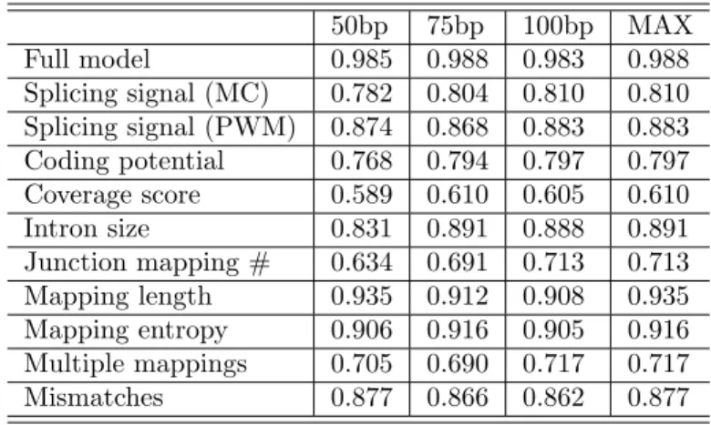
To demonstrate the contribution of each regressor in TrueSight to the final splice SJ clas-sification, we plotted Area Under Curve (AUC) values of the full model and each individual regressor on simulated datasets (described below) in Figure3. It is shown in Figure3 that the full model with all regressors achieves the best performance in selecting true positives from all candidate junctions.

2.2.7 Implementation

The core modules of TrueSight are written in C++, and are wrapped into a pipeline by Perl. TrueSight source code is freely available and can be downloaded from:

http://bioen-compbio.bioen.illinois.edu/∼yangli9/TrueSight/

2.3 Testing on real datasets

To assess accuracy of our algorithm and compare with existing tools, we selected RNA-seq data from human, fly, Arabidopsis, and C. elegans. (summarized in Table 1). For each species, we build a combined annotation of SJs, incorporating different sources, to achieve a better evaluation reference.

All predicted SJs are summarized into four classes (Table 4): (i) annotated junctions; (ii) junctions not annotated while both donor and acceptor splice sites are annotated; (iii) junctions with only one splice site is annotated; (iv) junctions where both splice sites are novel and not annotated.

(25)

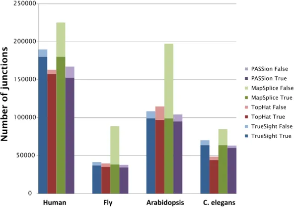
2010;Sultan et al.,2008), is still incomplete, several conclusions can be reasonably drawn. Junctions with both ends annotated (column Known introns in Table 3) are likely to be true junctions. For this type of splice forms, TrueSight and MapSplice are much more sensitive than TopHat and PASSion. We expect junctions with both novel splice sites (column Known introns in Table3) have high probability to be incorrect; for this category of junctions, MapSplice makes the largest number of false predictions, while other three tools reported much less misalignments. Figure4 shows the number of junctions detected as true and false by four tools on four datasets.

2.4 Testing on simulated datasets

We used Cufflinks (Trapnell et al., 2010) to estimate expression levels (RPKM) from the human embryonic stem cell (hESC) data on isoforms from UCSC knownGene model. We then used Maq (Li et al., 2008) (with an error rate of 0.02 for the Illumina reads) to generate simulation datasets with abundance proportional to hESC dataset based UCSC mRNA annotation, to build testing datasets more similar to real transcriptome sequencing data.

Three paired-end datasets with 20 million reads were generated, with 50bp, 75bp, and 100bp read length respectively. All four programs were tested with default settings (the number of mismatches is set as two). The results are summarized in Table 4. As shown in Figure 5, comparing with other three tools, TrueSight shows higher sensitivity for all datasets and this advantage is even more pronounced for low coverage junctions. In terms of specificity, TrueSight, TopHat and PASSion have approximately the same performance, which is substantially superior to MapSplice. This observation demonstrates that ’anchor-extension’ strategies without proper inference are likely to produce high false positives.

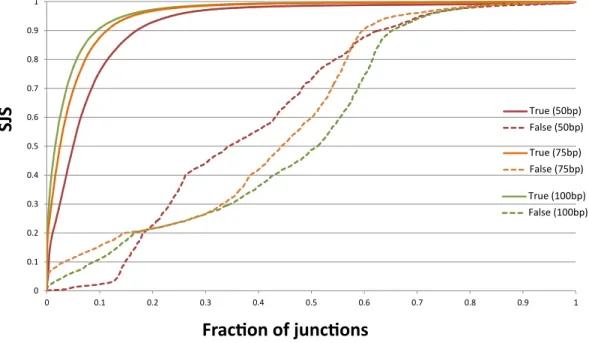
By plotting the TrueSightSJS distribution of both true and false junctions from three simulated datasets (Figure6), we observed distinctSJSpatterns for true and false junctions. 95% of true junctions haveSJS>0.5, while there are only 70% of false junctions withSJS

>0.5. Comparing theSJSdistribution between two datasets, we found that the power of TrueSight to separate true and false junctions is more obvious in samples with longer reads, which is consistent with the trend in sensitivity and specificity in Figure5.

(26)

al-most cannot find true non-canonical junctions for three datasets (consist with observations

in (Wang et al., 2010), even though it recovers the largest portion of semi-canonical

junc-tions in four tools, it also has the largest number of false predicjunc-tions. TrueSight has almost the same sensitivity but much higher specificity on non/semi-canonical junctions than Map-Splice.

2.5 Figures and Tables

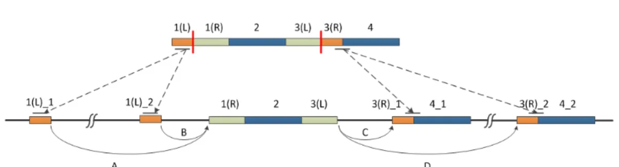
Figure 1: Gapped alignment. An IUM read is split into 4 segments(N = 4). Segment 2 and 4 can be fully mapped onto reference(segment 4 has two potential alignments, labeled as 4 1 and 4 2), while segment 1 and 3 cannot be aligned and are considered as junction spanning segments(M = 2). Segment 1 and 3 are split (shown by red solid lines) into left parts (1(L), 3(L)) and right parts (1(R), 3(R)), then we utilize segment 2 and 4 as ‘anchors’ and traverse each ‘path’(2→4 1 and 2→4 2) by searching gapped alignment for segment 1 and 3. There are four candidate gapped alignment for this read: A → C, A → D,

B→C andB→D. Logistic regression model integrating multiple features will score each candidate and infer the alignment with highest confidence for this IUM read.

Scale chr11: KLC2 KLC2 KLC2 KLC2 KLC2 1 kb 65782500 65783000 65783500 65784000 65784500 65785000 65785500 65786000 MapSplice TrueSight

UCSC Genes Based on RefSeq, UniProt, GenBank, CCDS and Comparative Genomics 0.143

0.165

Figure 2: Ambiguous splitting read supports alternative splicing (exon skipping here). 75bp read SRR065504.21341241.2 from human ESC sample (detailed description in real RNA-seq dataset section) has two distinct splitting patterns, labeled as blue and red. Mapping length on left and right side of both junctions is 11bp and 64bp respectively. The blue junction has higher score (0.165) than red junction (0.143) from TrueSight integrating both information from RNA-seq and DNA sequence, and supports an exon skipping event for gene KLC2, which is annotated by UCSC knowngene model. MapSplice reported the red junction and made a false alignment for this read, while Tophat failed to align this read, possibly resulting from the low coverage of this junction and the non-adjacency of the two exons involved.

(27)

Figure 3: Comparison of AUC values for each regressor. The full model utilizes spicing signal, coding potential and all RNA-seq regressors and has the best overall perfor-mance. AUC at 0.5 means a random guess.

0 50000 100000 150000 200000 250000 TrueSight False TrueSight True TopHat False TopHat True MapSplice False MapSplice True PASSion False PASSion True

Human Fly Arabidopsis C. elegans

Number of junctions

Figure 4: Evaluation of TrueSight, Tophat, MapSplice and PASSion on real datasets. We label ‘Known introns’ as true junctions and ‘both novel’ in Table 3 as false junctions.

(28)

0.3 0.4 0.5 0.6 0.7 0.8 0.9 1 1 2 3 4 5 6 7 8 9 10 TrueSight TopHat MapSplice PASSion 0.3 0.4 0.5 0.6 0.7 0.8 0.9 1 1 2 3 4 5 6 7 8 9 10 TrueSight TopHat MapSplice PASSion 0.4 0.5 0.6 0.7 0.8 0.9 1 1 2 3 4 5 6 7 8 9 10 TrueSight TopHat MapSplice PASSion 0.4 0.5 0.6 0.7 0.8 0.9 1 1 2 3 4 5 6 7 8 9 10 TrueSight TopHat MapSplice PASSion 0.5 0.55 0.6 0.65 0.7 0.75 0.8 0.85 0.9 0.95 1 1 2 3 4 5 6 7 8 9 10 TrueSight TopHat MapSplice PASSion 0.5 0.55 0.6 0.65 0.7 0.75 0.8 0.85 0.9 0.95 1 1 2 3 4 5 6 7 8 9 10 TrueSight TopHat MapSplice PASSion (A) 50bp (B) 75bp (C) 100bp

Junction Coverage (log2)

S e ns i tiv ity S e ns i tiv ity S e ns i tiv ity Specificity Specificity Specificity

Figure 5: Evaluation of TrueSight, Tophat, MapSplice and PASSion on sim-ulated datasets. On each dataset, the sensitivity and specificity is plotted as function of junction coverage. The sensitivity is the ratio of detected positive junctions over all junctions covered by simulated reads; specificity is the ratio of positive junctions over all reported ones.

(29)

0 0.1 0.2 0.3 0.4 0.5 0.6 0.7 0.8 0.9 1 0 0.1 0.2 0.3 0.4 0.5 0.6 0.7 0.8 0.9 1 True (50bp) False (50bp) True (100bp) False (100bp) True (75bp) False (75bp)

Fraction of junctions

SJ

S

Figure 6: Distribution of TrueSight scores on true and false junctions. X-axis is the fraction of true/false junctions under certain SJS. Overall, negative junctions have much lower scores than positive ones. TrueSight has higher power to separate true and false junctions in dataset with longer reads.

(30)

Table 1: Real datasets description

Species Length (bp) Pair (M) SRA accession # Reference Annotations

Human 75 24.28 SRR065504 hg19 refseq, ensemble

spliced EST UCSC knowngene

Fly 76 13.60 SRR042297 dm3 flybase r5.42

Arabidopsis 76 20.90 SRR360205 TAIR9 TAIR9

C. elegans 102 12.24 SRR359066 ce10 refseq, ensemble

Real datasets for evaluation of four tools. All datasets are paired-end RNA-seq reads, with length, coverage and SRA accession listed. The genome reference used in alignments and annotation references for SJs evaluation have also been listed.

Table 2: AUC value for each regerssor and full TrueSight model on simulated datasets 50bp 75bp 100bp MAX Full model 0.985 0.988 0.983 0.988 Splicing signal (MC) 0.782 0.804 0.810 0.810 Splicing signal (PWM) 0.874 0.868 0.883 0.883 Coding potential 0.768 0.794 0.797 0.797 Coverage score 0.589 0.610 0.605 0.610 Intron size 0.831 0.891 0.888 0.891 Junction mapping # 0.634 0.691 0.713 0.713 Mapping length 0.935 0.912 0.908 0.935 Mapping entropy 0.906 0.916 0.905 0.916 Multiple mappings 0.705 0.690 0.717 0.717 Mismatches 0.877 0.866 0.862 0.877

50bp, 75bp and 100bp simulated datasets are used to evaluate each regressor and full model. The maximum value for each regressor is in Figure3

(31)

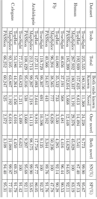
Table 3: Testing on real datasets Dataset T o ols T otal Both ends kno wn One no v el Both no v el SN(%) SP(%) Kno wn No v el Human T rueSigh t 225,535 180,156 11,368 24,238 9,773 99.90 95.67 T opHat 192,939 157,625 8,613 14,494 5,541 87.40 97.13 MapSplice 267,932 180,337 13,191 29,376 45,028 100 83.19 P ASSion 185,399 152,654 5,668 12,448 14,629 84.65 92.11 Fly T rueSigh t 46,656 37,191 568 4,481 4,416 96.44 90.53 T opHat 44,080 35,532 733 3,530 4,285 92.14 90.28 MapSplice 96,204 38,565 777 6,626 50,236 100 47.78 P ASSion 40,566 34,617 443 2,162 3,344 89.76 91.76 Arabidopsis T rueSigh t 119,729 99,307 691 10,596 9,135 100 92.37 T opHat 127,311 97,093 2,644 9,816 17,758 97.77 86.05 MapSplice 212,713 99,207 1,218 14,113 98,175 99.90 53.85 P ASSion 108,429 95,016 538 3,668 9,207 95.68 92.11 C.elegans T rueSigh t 77,154 63,823 1,211 5,499 6,621 100 91.42 T opHat 54,186 44,264 1,456 4,016 4,450 69.35 91.79 MapSplice 92,105 63,807 1,192 6,018 21,088 99.97 77.10 P ASSion 66,252 60,247 525 2,372 3,108 94.40 95.31

All mapped SJs from different tools are categorized into four classes as described in the main text. Sensitivity is the fraction of ‘known introns’ to the largest number of ‘known introns’ discovered by one method, thus the most exhaustive method is defined to have 100% sensitivity. Specificity is calculated by dividing ‘both novel’ junctions over ‘total’ number of junctions reported.

(32)

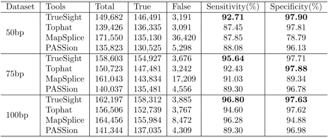
Table 4: Testing on simulated datasets

Dataset Tools Total True False Sensitivity(%) Specificity(%) 50bp TrueSight 149,682 146,491 3,191 92.71 97.90 Tophat 139,426 136,335 3,091 87.45 97.81 MapSplice 171,550 135,130 36,420 87.85 78.79 PASSion 135,823 130,525 5,298 88.08 96.13 75bp TrueSight 158,603 154,927 3,676 95.64 97.71 Tophat 150,723 147,481 3,242 92.43 97.88 MapSplice 161,043 143,834 17,209 91.03 89.34 PASSion 140,037 135,481 4,556 89.30 96.78 100bp TrueSight 162,197 158,312 3,885 96.80 97.63 Tophat 156,506 152,739 3,767 94.60 97.62 MapSplice 164,456 155,984 8,472 96.28 94.88 PASSion 141,344 137,035 4,309 89.30 96.98

Sensitivity is fraction of true junctions in all junctions covered by RNA-seq; Specificity is fraction of true junctions of all predicted junctions. Best sensitivity and specificity are highlighted.

Table 5: Semi-canonical and Non-canonical junctions

Dataset Tools Semi-canonical Non-canonical

SN SP SN SP 50bp TrueSight 71.40 85.94 10.74 8.45 TopHat 74.23 61.15 0.67 30.00 MapSplice 54.97 64.46 6.04 4.29 PASSion 81.63 80.41 11.41 0.83 75bp TrueSight 77.10 85.86 12.42 13.23 TopHat 87.65 56.46 0.65 17.31 MapSplice 75.16 63.56 13.72 6.85 PASSion 82.05 92.85 11.76 3.04 100bp TrueSight 80.27 88.02 12.58 14.87 TopHat 89.99 50.60 0 16.98 MapSplice 83.72 73.67 15.72 10.73 PASSion 82.45 94.83 12.58 3.38

Semi-canonical and Non-canonical junctions identified by TrueSight, TopHat, MapSplice and PASSion on 50bp, 75bp and 100bp simulation datasets. TopHat and PASSion identified largest number of semi-canonical junctions, while TrueSight and PASSion achieve the highest specificity. When searching non-canonical junctions which have no specific splice site signal, TrueSight and Mapsplice show approximately the same SN and SP. Few correct non-canonical junctions were found by TopHat, while PASSion has extremely low SP.

(33)

Chapter 3

Honey bee transcriptome

analysis

3.1 Dataset

190 million 100bp paired-end reads are obtained through cDNA sequencing on ten dis-sected honey bee (Apis mellifera) fat body tissues, achieving approximately 1,400X average coverage on current bee gene model.

Honey bees were maintained at the University of Illinois Beekeeping Facility according to standard beekeeping procedures. Bees for RNA-seq were from colonies of single drone inseminated queens to reduce genetic variation for deep sequencing.

TrueSight program was running with default parameters and mapped the RNA-seq reads from each sample onto honey bee assembly 4.

3.2 Improving GLEAN model

The honey bee GLEAN consensus gene set (Elsik et al., 2007) is created by integrating multiple gene lists, with a balanced sensitivity and specificity. However, we consider this model too conservative in the sense that AS of honey bee is currently under estimated. With the aid of deep RNA-seq data, we apply TrueSight to find SJs that are essential for AS identifications and modify the GLEAN gene model with following procedures.

3.2.1 Transcribed Islands

To obtain reliable ‘transcribed islands’ on bee genome, we filtered TrueSight alignments for 10 samples by only retaining best alignment (smallest number of mismatches for full alignment; highest TrueSight score for gapped alignment) for each RNA-seq read. After the filtering, we get digital read counts for each base on bee genome and search for ‘transcribed islands’ with following criteria: (i) at least 5X coverage on each base of the island; (ii)

(34)

transcribed island should be longer than 50bp.

The boundary for ‘transcribed islands’ identified at this stage is chosen independently from any splicing signals or SJs inferred by TrueSight, and will be further determined by the following gene model modification process.

All transcribed islands are compared with exons already in GLEAN gene model and only those completely non-overlapping islands are retained for identifying novel exons or transcripts.

3.2.2 TrueSight SJ

SJs from independent TrueSight runnings on 10 samples were clustered together, by assign-ing the highest TrueSight score for each junction, if it was detected in multiple samples. SJs with score larger than 0.5 were retained as TrueSight SJs and will be utilized to modify current GLEAN model.

3.2.3 Improving GLEAN gene model with iterative algorithm

Initiation

By comparing TrueSight SJ with SJ inferred from GLEAN gene model (model0_{, we define} a set of exons and SJs as a primary gene model), TrueSight SJ can be categorized into four subsets: (i) known SJ, which are already in model0; (ii) novel SJ with both splice sites known (novel00), which are evidences for skipping exons, since they link non-adjacent exons; (iii) novel SJ with only one known splice site (novel0

1); (iv) novel SJ with two novel splice sites (novel0

2). Iteration

Intth(t≥1) iteration:

• Adding new link (SJ) to existing exons withnovelt₀−1

SJ in novelt₀−1 provide novel links to existing exons in modelt−1_{, and are strong} supports for cassette exons. novel₀t−1is added intomodelt−1_{to construct new version} of gene modelmodelt

(35)

The original junction linking two exons (a∼b;c∼d) isb∼c, and if there is junction innovelt₁−1: b0_∼_c_{, such that}_k_b0₋_b_k_<_200,_b0_{> a}_{, exon}_a_∼_b_{would have alternative} boundary a∼b0; if there is junction innovelt₁−1: b∼c0 , such thatkc0−ck <200,

c0< d, exonc∼dwould have alternative boundaryc0∼d.

SJs used in modifying exon coordinates should be on the same strand as the exon. And both the SJs and modified exon boundaries are added into modelt_.

All junctions in novel₁t−1, which are not utilized in modifying exon boundaries and not added intomodeltare categorized asnovelt−1. And also junctions innovel₂t−1are added intonovelt−1.

Junctions in the new setnovelt−1 _{are compared with}_modelt _{and categorized into} _novelt

0,

novel₁t andnovel₂t, which are used in the (t+ 1)thiteration.

Termination

The modification process would terminate at Tth iteration when there is no junction in

novel0T. SJs innovelT1 andnovelT2 are utilized for adding new exons/transcripts tomodelT After five iterations, the number of SJs in original GLEAN gene model has increased from 53,884 to 66,847. And these newly added junctions are signals for two types of AS: cassette exons (CE) and alternative exon boundaries (AB).

3.2.4 Adding new exons/transcripts

To be conservative in adding novel exons/transcripts into modified GLEAN model, we only usenovelT

1 andnovelT2 with TrueSight score larger than 0.9.

• Adding new exons/transcripts withnovelT₁

For exon a ∼b, if there is a junction in novelt₁−1: b ∼ p0, such that we can find a Transcribed Island (p∼q), satisfying that kp0−pk <100,p0 < q, we can label the Transcribed Island (p0∼q) as a new exon, with one boundary (p0) fixed and the other (q) undetermined.

Symmetrically, for exona∼b, if there is a junction innovel₁t−1: q0∼a, such that we can find a Transcribed Island (p∼q), satisfying that kq0−qk <100,q0 > p, we can label the Transcribed Island (p∼q0) as a new exon, with one boundary (q0) fixed and the other (p) undetermined.

(36)

The new exons identified in this process are in two subsets: (i) new exons with both boundaries fixed, for both ends of these exons are linked to known exons by junctions in novelT

1. (ii) new exons with only one end defined (Novel Terminal Exons). These Novel Terminal Exons are either first/last exons of the whole transcripts, or linking to further novel exons by SJ innovelT

2.

• Adding new exons/transcripts withnovelT

2 For a SJ in novelT

2 : q0 ∼p0, if there are two Transcribed Islands (p1 ∼q1,p2 ∼q2), such that: q1 < p2, kq0 −q1k <100, q0 > p1, kp0−p2k <100, p0 < q2, we can link these two Transcribed Islands together by the junctionq0∼p0.

There are two outcomes of this novel exon adding process: (i) novel multi-exon transcripts in inter-genic regions of GLEAN model; (ii) novel exons might be linked to Novel Terminal Exons identified in previous process, thus these novel exons serve as new Novel Terminal Exons for known gene.

Comparing with the original GLEAN model, 5,873 new exons are added and the number of SJs in the modified model has increased from 53,884 to 70,022. These newly added junctions are potential signals for various types of AS. We have identified 2,803 novel multi-exon transcripts in inter-genic regions of GLEAN model.

3.3 Alternative splicing of a sex determination gene

(

fruitless

)

The fruitless is a master regulator of sex determination in D. melanogaster (Demir and

Dickson,2005), as well as in some other species (Bertossa et al.,2009;Clynen et al.,2011).

fruitlessis one of the largest and most complex genes inD. melanogaster, with four promoters and four alternative 3’ ends within its gene model that can generate a large number of different transcripts. Through sex-specific splicing, isoforms with male-specific promoters are essential in male courtship behavior; male flies lacking these isoforms are sterile (Villella

and Hall,2008).

By contrast to the wealth of information in Drosophila, thefruitlessgene model in honey bee was poorly built, but with our enhanced annotation, a detailed picture of fruitless AS has been revealed. As shown in Figure8, thefruitlessgene model in honey bee is much more

(37)

complicated than previously annotated, with three promoters (first exons), five alternative 3’ ends and exon 1 as a cassette exon. The modified gene model is now similar to thefruitless gene model in D. melanogaster which has four promoters and four alternative 3’ ends, even though these two species have 300 million years of evolutionary distance. Theoretically there are 20 different isoforms for the honey bee fruitless gene, harboring 16 ORFs, in which 15 ORFs are found to have both BTB and ZNF domains.

3.4 Quantitative analysis

RNA-seq has been shown to be very effective in revealing AS of transcripts (Pan et al.,

2008; Gonzalez-Porta et al., 2012). We used a high-coverage RNA-seq data set of adults’

fat cell transcriptomes and TrueSight to perform quantitative analysis of AS and study the correlation between AS and various factors.

There are four principal types of AS (Nilsen and Graveley, 2010): 1) Retaining Intron (RI), in which an intron may be retained as part of a mature transcript or spliced out; 2) exon skipping, in which a Cassette Exon (CE) may be included or not in transcripts; 3) alternative use of splice sites (donor/acceptor), leading to Alternative exon Boundaries (AB); and 4) alternative Terminal Exons (ATE), in which Alternative First Exons (AFE) or Alternative Last Exons (ALE) are used.

AS operates as a combinatory mechanism, in which splice site strength, exon/intron architecture, splicing enhancers and silencers, and RNA secondary structures contribute to a gene’s final splicing outcomes (Hertel,2008). In addition, it recently has been shown that epigenetic regulation also is involved in AS (Luco et al., 2011,2010). We studied the link between the splicing ratio and various factors, including the exon-intron model, splice site strength and methylation pattern, for each AS subtype.

3.4.1 Retaining Intron

From 59,674 honey bee introns on 9,355 multi-exon genes, we identified 10,095 (16.9%) RI on 4,482 (47.9%) genes. We define one intron as an RI in transcriptome if each base of the intron has>5X coverage from TrueSight RNA-seq alignments.

(38)

adjacent exonsa∼p,q∼d, itsRI inclusion ratiois calculated by the following equation

Cov(p, q)

Cov(a, p) +Cov(q, d)

WhereCov(x, y) =

Py

i=xnumber of reads mapped onto i

y−x .

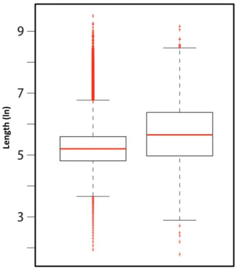
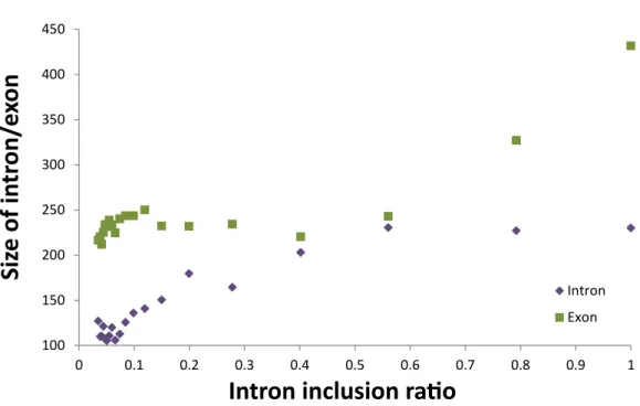
Overall, RIs are significantly shorter than non-retained introns (Fig 9), which is consis-tent with observation in rice (Zhang et al.,2010). We also observe that RIs with relatively larger intron (and adjacent exon) sizes have a greater tendency to be retained (Fig 10), which supports the intron splicing model, such that relatively longer introns are relatively harder to be identified in intron splicing mechanism (Berget,1995).

For RIs with higher inclusion rate (more likely retained), we have found their donor/accepter splice sites are weaker than those RIs more likely to be successfully spliced out in transcripts (Fig11). When RI inclusion ratiois low, the strong donor and acceptor sites flanking the RI would help it be successfully recognized and spliced out in most transcripts for the AS gene. This observation also supports the intuitive hypothesis that RI is flanked by relatively weak splice sites which are occasionally not recognized by splicesome (Stamm et al.,2000). Similar observation is reported in Arabidopsis (Marquez et al.,2012) and a much rougher estimate of the correlation between splice site strength and RI inclusion ratio was reported in a work based on human cDNA counts (Sakabe and de Souza,2007).

3.4.2 Cassette Exon

In 69,799 bee exons, 2,077 (2.98%) are cassette exons (CEs), which originate from 1,585 (17.0%) genes. The average size of CEs is 245bp, smaller than the average size for all bee exons (272bp, two tailed t-test p value < 1e−10, Fig 14). Similar to other species such as human and mouse (Sorek et al., 2004a,b; Daines et al., 2011), the lengths of CEs are enriched as 3N (bp), when comparing with other bee exons (Chi-square test p value is less thane−10_{, Fig}₁₃_{). The 3-periodic enrichment would help preserve the reading frame and} might be conserved during evolution.

To study CE, we defineCE inclusion ratio: for an CE with coordinatesp∼qand two adjacent constitutive exonsa∼b, c∼d,CE inclusion ratiois calculated by

Cov(p, q)

(39)

WhereCov(x, y) =

Py

i=xnumber of reads mapped onto i

y−x .

By performing conservation analysis to proteins in Drosophila and human, we observed that, CEs with largerCE inclusion ratio are presumably more conserved than those CEs more often to be skipped. To study the mechanism underlying exon skipping, we plotted the donor/accepter splice site strengths againstCE inclusion ratio(Fig15) and found that, CEs with larger inclusion rate have stronger accepter sites, however, donor sites strength seems to have no impact on CEs.

CpG (o/e) is a computational metric measuring the DNA methylation on an evolution-ary time scale, under the hypothesis that methylated cytosines are hypermutable and the low CpG (o/e) value implies the depletion of CpG dinucleotides during evolution and the potential hyper-methylation (Gardiner-Garden and Frommer, 1987). On the other hand, high CpG (o/e) would be a reasonable hint for hypo-methylation.

The CpG (o/e) is defined as

CpG(o/e) = PCpG

PC∗PG

where PCpG, PC, and PG measure the frequencies of observing CpG dinucleotides, C

nu-cleotides, and G nunu-cleotides, respectively.

CpG (o/e) and actual methylation pattern have good correlation in previous works on various species, including honey bee (Elango et al.,2009;Lyko et al.,2010).

We have found that the average CpG (o/e) for CEs is larger than average CpG (o/e) for all bee exons (two tailed t test P-value< e−10, shown in Fig 12), implying that CEs have relatively lower methylation level (hypo-methylated).

By plotting average CpG (o/e) versus averageCE inclusion ratio for 20 bins described previously (Fig12), we observe a strong negative correlation between CpG (o/e) and CE inclusion ratio. The methylation level for highly included CEs is similar to the level for all exons, while those rarely included CEs tend to have much lower methylation level.

3.4.3 Alternative exon Boundary

Alternative exon Boundary (AB) is previously reported as most dominant AS subtype in various species (Daines et al., 2011). In total, there are 2,684 alternative donor (5’) sites and 5,405 alternative acceptor (3’) sites on 6,994 exons from 4,115 genes of honey bee,

(40)

making almost half of bee genes producing multiple isoforms with AB. Interestingly, the 2-fold enrichment of alternative 3’ sites to 5’ sites is consistent with previous findings in Arabidopsis (Marquez et al.,2012). We observe 3-periodic enrichment for nearby AB splice sites (Fig 17). The enrichment of 3-fold distances has been reported previously (Daines

et al., 2011). Interestingly, 4bp gap dominates in alternative donor sites, which disturbs

original ORFs. For acceptor sites, the 3bp gap in accepter sites (NAGNAG tandem splice sites), producing splice variants differs by only one amino acid, is mostly abundant in honey bee and has also widespread in human genome, with more than 5% human genes are experimentally confirmed to contain NAGNAG tandem sites(Hiller et al. 2004). NAGNAG tandem sites are functional related to several human diseases (Hinzpeter et al.,2010) and under specie-specific and tissue-specific regulation (Hiller et al.,2004;Bradley et al.,2012). We plotted motif logos of 3/4/5bp AB sites for both donors and acceptors (Fig18).

To study AB, we defineAB splicing ratio. For three continuous exons (a∼b,p∼q,c∼ d) on the forward strand, exonp∼q has alternative acceptor splice site p’ and alternative donor splice site q’.

TheAB splicing ratiofor the acceptor sites, which describes the expression ratio of minor (less used) acceptor sites to major (more used) ones, is:

min(N(b∼p), N(b∼p0))

max(N(b∼p), N(b∼p0₎₎

AB splicing ratiofor the donor sites, which describes the expression ratio of minor donor sites to major ones, is:

min(N(q∼c), N(q0∼c))

max(N(q∼c), N(q0_∼_c₎₎

WhereN(x∼y) =number of reads mapped onto junction x∼y.

Since most AB splice sites are co-located, the competition between alternative splice sites would determine final expression ratio for each isoform (Xia et al.,2006;Yu et al.,2008). To test this hypothesis, we plotted the relative splice site strength for both alternative donor and acceptor sites (Fig19) againstAB splicing ratio. We can observe that the expression ratio of two splice sites (weak/strong) goes up when their relative splice site strength goes down (strong-weak), which coincides with the hypothesis that nearby alternative splice sites are in a competing mode, such that relative stronger site would have higher probability to be used in the splicing mechanism.

(41)

To look at specific ABs, we define AB inclusion ratio, measuring inclusion ratio of alternative exon boundaries. For the same three exons listed in last section, theAB inclusion ratioof regionmin(p, p0)∼max(p, p0) is:

N(b∼min(p, p0))

N(b∼p) +N(b∼p0₎ For regionmin(q, q0)∼max(q, q0):

N(max(q, q0)∼c))

N(q∼c) +N(q0_∼_c₎

To study the relation between methylation of AB region with its AB inclusion ratio, we plotted average CpG (o/e) versus average AB inclusion ratio (Fig 16). We can observe from the figure that regions rarely included in transcripts have greater tendency to be hypo-methylated, which supports our observations for CEs.

3.4.4 Alternative Terminal Exon

Both AFEs and ALEs are categorized as ATEs. For honey bee, we identified that ∼5% genes have AFEs and ∼ 11% genes have ALEs (Table 6). For each pair of ATEs, we categorize it into one of five categories based onATE splicing ratio. TheATE splicing ratio measures the expression ratio of minor ATEs to major ones. Note that we only consider AFEs/ALEs directly linking to the same accepter/donor site of a constitutive exon in this analysis. The calculation is similar to formulas forAB splicing ratio, using minor junction mappings over major junction mappings.

We have found that, for both ATEs with low splicing ratio (<0.2), the splice site strength for major ATEs are significantly stronger than minor ones (P-value<0.001), while for those with large splicing ratio (0.8-1), there is no significant strength difference for the splice site between major and minor ATEs (Fig20). As we have observed in CE and AB, rarely used exon sequences are likely to be theoretically hypo-methylated. We can make the assumption on minor ATEs which are rarely included in transcripts. As shown in Fig21, the minor ATEs with low splicing ratio (<0.2) have significantly higher CpG(o/e) than major ATEs (P-value<0.001) and this trend cannot be observed for ATEs in high splicing ratio category (0.8-1).

(42)

(43)

3

5

7

9

Annotated exons New exons

Leng

th (ln)

Figure 7: Size distribution of exons annotated in GLEAN model and detected from RNA-seq.

(44)

Figure 8: Alternative splicing pattern in fruitless revealed by TrueSight.(A) Number of reads (from 10 samples) mapped onto each base infruitlessgene region is plotted. (B) SJs with TrueSightSJSlarger than 0.5 are plotted. Black junctions are those annotated in GLEAN model; red ones are junctions with one splice site annotated; blue junction has both splice sites annotated, and this junction supports the skipping; orange junctions have both ends novel. (C) The current GLEAN model offruitless. (D) The potential gene model by modifying GLEAN model with TrueSight SJs shown in (B). Red boxes are internal exons (BTB domain and connector domain, labeled as 1, 2, 3), while blue boxes are alternative starting exons (labeled as P1, P2, P3) and green ones are alternative last exons (harboring ZNF, labeled as A, B, C, D, E). Dominant SJs (with largest RNA-seq mapping numbers) are shown in red lines and other alternative ones are presented by black lines. Note that exon P3 has two alternative donor splice sites, with 2bp upstream (13 reads mapped on) and 19bp downstream (11 reads mapped on) of the major donor site.

(45)

0 5000 10000 15000 20000 25000 30000 35000 40000 0 2000 4000 6000 8000 10000 12000 5.5 6 6.5 7 7.5 8 8.5 9 9.5 10 Retaining introns All introns

log2 of intron size

Number of r

et

aining in

tr

ons

Number of all bee in

tr

ons

Figure 9: Distribution of RI sizes. Kernel density (generated by Matlab) plot for the lengths of all bee introns and RIs. The average size of RIs is 146bp, differing from average size 1,399bp for all bee introns (two tailed t test P-value<1e−10_).

100 150 200 250 300 350 400 450 0 0.1 0.2 0.3 0.4 0.5 0.6 0.7 0.8 0.9 1 Intron Exon

Intron inclusion ratio

Siz

e of in

tr

on/

ex

on

Figure 10: Size of RI and average size of adjacent exons versus RI inclusion ratio. Kernel density (generated by Matlab) plot for the lengths of all bee introns and retained introns. The average size of retained introns is 146bp, differing from average size 1,399bp for all bee introns (two tailed t test P-value<1e−10_).

(46)

2 2.5 3 3.5 4 4.5 5 5.5 6 0 0.2 0.4 0.6 0.8 1 Donor Acceptor

Intron inclusion ratio

Splice sit

e s

tr

eng

th

Figure 11: Motif strength of RI splice sites. Both donor and acceptor splice sites strengths are plotted against intron inclusion ratio in 20 RI bins. There is a strong negative correlation between splice site strength and RI inclusion rate.

Figure 12: Average CpG (o/e) versus CE inclusion ratio. CEs with larger inclusion rate tend to have smaller CpG (o/e), implying higher methylation level comparing with rarely included CEs. Both average CpG (o/e) levels for CEs and all bee exons are shown as horizontal lines.

(47)

0 0.01 0.02 0.03 0.04 0.05 3N 3N+1 3N+2

Skipping exon length

Ra

tio t

o all e

xons

Figure 13: Distribution of CE numbers on their divisibility by 3. -periodic exons (3N) are enriched comparing to other two categories (3N+1, 3N+2) and chi-square test p value is less than e−10 _{for 3-periodic and non-3periodic exons (} _χ2 _{= 180}_._{878 with one} degree of freedom). The 3-periodic enrichment would help preserve the reading frame and might be conserved during evolution.

0 50 100 150 200 250 300 0 1 2 3 4 5 6 7 8 9 10 0 100 200 300 400 500 600 Skipping exons All exons Number of skipping e xons

Number of all bee e

xons

Exon size (bp)

Figure 14: Distribution of CE sizes. Kernel density (generated by Matlab) plot for the lengths of all bee exons and CEs. The average size of CEs is 245bp, smaller than the average size for all bee exons which is 272bp (two tailed t test P-value<1e−10_).

(48)

2.5

3

3.5

4

4.5

5

5.5

0

0.2

0.4

0.6

0.8

1 Accepter

Donor

Splice sit

e s

tr

eng

th

Exon inclusion ratio

Figure 15: Motif strength of CE splice sites. CEs with high acceptor strength have higherCE inclusion ratio, while donor sites strength does not show correlation with theCE inclusion ratioof CEs..

0

0.2

0.4

0.6

0.8

1

1.2

1.4

1.6

1.8

0

0.2

0.4

0.6

0.8

1 Average CpG (o/e) of all bee exons

Average CpG (o/e) of each bin

AB inclusion rate

CpG (o/

e)

Figure 16: Average CpG (o/e) versus AB inclusion ratio. To study the relation between methylation status (computational) of AB region with its inclusion rate, we sort the overall AB list, including both donor and acceptor boundaries, according to theirAB inclusion ratiodescribed in main text and get 20 equal size bins. CpG (o/e) is negatively correlated withAB inclusion ratio. AB regions with low inclusion ratio are presumably to be hypo-methylated.

Novel methods in transcriptome analysis using RNA-seq