University of Wollongong University of Wollongong
Research Online
Research Online
Centre for Statistical & Survey Methodology
Working Paper Series Faculty of Engineering and Information Sciences
2008
Spatial M-quantile Models for Small Area Estimation
Spatial M-quantile Models for Small Area Estimation
N. Salvati University of Pisa M. Pratesi University of Pisa N. Tzavidis University of Manchester R. ChambersUniversity of Wollongong, [email protected]
Follow this and additional works at: https://ro.uow.edu.au/cssmwp
Recommended Citation Recommended Citation
Salvati, N.; Pratesi, M.; Tzavidis, N.; and Chambers, R., Spatial M-quantile Models for Small Area Estimation, Centre for Statistical and Survey Methodology, University of Wollongong, Working Paper 15-08, 2008, 16p.
https://ro.uow.edu.au/cssmwp/12
Research Online is the open access institutional repository for the University of Wollongong. For further information contact the UOW Library: [email protected]
Copyright © 2008 by the Centre for Statistical & Survey Methodology, UOW. Work in progress, no part of this paper may be reproduced without permission from the Centre.
Centre for Statistical and Survey Methodology
The University of Wollongong
Working Paper
15-08
Spatial M-quantile Models for Small Area Estimation
Spatial M-quantile Models for Small Area Estimation
Nicola Salvati, Monica Pratesi
Dipartimento di Statistica e Matematica Applicata all’Economia, Università di Pisa, via Ridolfi, 10 – 56124 Pisa,
[email protected], [email protected]
Nikos Tzavidis
Centre for Census and Survey Research,
University of Manchester, Manchester M13 9PL, UK, [email protected]
Ray Chambers
Centre for Statistical and Survey Methodology,
University of Wollongong, NSW 2522, Australia, [email protected]
Abstract: In small area estimation direct survey estimates that rely only on area-specific data can exhibit large sampling variability due to small sample sizes at the small area level. Efficient small area estimates can be constructed using explicit linking models that borrow information from related areas. The most popular class of models for this purpose are models that include random area effects. Estimation for these models typically assumes that the random area effects are uncorrelated. In many situations, however, it is reasonable to assume that the effects of neighbouring areas are correlated. Models that extend conventional random effects models to account for spatial correlation between the small areas have been recently proposed in literature. A new semi-parametric approach to small area estimation is based on the use of M-quantile models. Unlike traditional random effects models, M-quantile models do not depend on strong distributional assumptions and are robust to the presence of outliers. In its current form, however, the M-quantile approach to small area estimation does not allow for spatially correlated area effects. The aim of this paper is to extend the M-quantile approach to account for such spatial correlation between small areas.
Keywords: Quantile regression, Robust models, Spatial correlation, Weighted least squares
1. Introduction
In small area estimation direct survey estimates that rely only on area-specific data can exhibit large sampling variability due to small sample sizes. In order to increase the efficiency of small area estimates, it is common practise to construct small area estimates using explicit linking models that borrow information from related areas. The most popular class of these are models that include random area effects to account for between area variation beyond that explained by the auxiliary
variables in the model. Estimation for these models is typically carried out assuming that the random area effects are uncorrelated (Ghosh and Rao 1994; Rao 2003). In many situations, however, it is reasonable to assume that the effects of neighbouring areas – where neighbourhood is often defined in terms of a contiguity criterion - are correlated with the correlation decaying to zero
as between area distance increases (Petrucci et al. 2005). In such cases the assumption of spatial
independence of the random area effects becomes questionable. The problem of accounting for spatial correlation between the small areas has been recently tackled by extending the model of
Battese et al. (1988) using a Simultaneously Autoregressive (SAR) process (Salvati 2004; Petrucci
and Salvati 2006).
Chambers and Tzavidis (2006) have proposed a new approach to small area estimation that is based on the use of M-quantile models. Unlike traditional random effects models, M-quantile models do not depend on strong distributional assumptions and are robust to the presence of outliers. In its current form, however, the M-quantile approach to small area estimation does not allow for spatially correlated area effects. The aim of this paper is to extend the M-quantile approach to account for spatial correlation between small areas.
The paper is organized as follows. In section 2 we review random effects models that allow for spatially correlated random effects. In section 3 we propose an extension of the M-quantile approach to account for spatial correlation between the small areas. In section 4 we demonstrate
usefulness of this framework through Monte Carlo simulation studies. The main focus of the
comparisons is between the Spatial M-quantile and M-quantile models. In section 5 we present an application of spatial M-quantile models for estimating the average and median production of olives at the level of Local Economy System (LES) in Tuscany. Finally, in section 6 we summarise our main findings.
2. Small Area Models with Spatially Correlated Random Effects
Let xi be a known vector of pauxiliary variables for each population unit j in small area i and
assume that information for the variable of interest y is available only on the sample. The target is to
use these data to estimate various area specific quantities. The most popular models used for this purpose are mixed effects models, i.e. models with random area effects. A linear mixed effects model has the following form:
yij =xij T!+
zijui+"ij, j=1…ni, i=1…m (2.1)
where ui denotes a random area effect that characterizes differences in the conditional distribution
in the population and !ij is the error term associated with the j-th unit within the i-th area.
Conventionally, ui and !ij are assumed to be independent and normally distributed with mean zero
and variances 2
u
! and 2
!
" respectively (Battese et al. 1988).
Model (2.1) can be extended to allow for correlated area effects. Let the deviations v from the
fixed part of the model xT! be the result of an autoregressive process with parameter ! and
proximity matrix W (Cressie 1993; Anselin 1992), i.e.
v=!Wv+u"v=(I#!W)#1u (2.2)
where I is m!m identity matrix. Combining (2.1) and (2.2), with ! independent of v, the model
with spatially correlated errors can be expressed as y=xT!+
Z(I"#W)"1
u+$. (2.3)
The error term v then has the m!m Simultaneously Autoregressive (SAR) dispersion matrix:
G=!u2
I"#WT
(
)
(
I"#W)
$% &'"1. (2.4)
The W matrix describes the neighbourhood structure of the small areas whereas ! defines the
strength of the spatial relationship among the random effects associated with neighbouring areas. For ease of interpretation, the general spatial weight matrix is defined in row standardized form in
which case ! is referred to as the spatial autocorrelation parameter (Banerjee et al. 2004). Under
(2.3), the Spatial Best Linear Unbiased Predictor (Spatial BLUP) estimator of the small area parameters and its empirical version (SEBLUP) are obtained following Henderson (1975). The
SEBLUP estimator of the mean for small area i, yi, is
ˆ yi =xi T!ˆ+ bi T"ˆ u 2 I#$ˆWT
(
)
(
I#$ˆW)
%& '(#1ZT ˆ ")2In +Z"ˆu 2 I#$ˆWT(
)
(
I#$ˆW)
%& '(#1 ZT{
}
#1 (ys#x T!ˆ ) (2.5) where xiT denotes a known area specific vector of population means for the auxiliary variables,
s y is a n!1 vector of the sampled observations, !ˆu2
, ˆ!"2, ˆ# are asymptotically consistent estimators of
the parameters obtained by Maximum Likelihood (ML) or Restricted ML (REML) method; bi
T is a
m !
1 vector (0,0…0,1,…0) with value 1 in the i-th position.
The mean squared error (MSE) of SEBLUP and its estimator are obtained following the results of Kackar and Harville (1984), Prasad and Rao (1990) and Datta and Lahiri (2000). More
estimation of the random effects (g1), the estimation of ! (g2) and the estimation of the variance
components (g3). Note that, due to the introduction of the additional parameter !, the component
g3 of the MSE is not the same as in the case of the traditional EBLUP estimator (Saei and Chambers
2003; Singh et al. 2005; Petrucci and Salvati 2006).
3. Spatial M-quantile Models for Small Area Estimation
Chambers and Tzavidis (2006) have proposed a new approach to small area estimation that is based
on modelling the M-quantiles of the conditional distribution of the study variable (y) given the
covariates (Breckling and Chambers, 1988). Unlike mixed effects models, which assume that the
variability associated with the conditional distribution of y given x can be at least partially
explained by a pre-specified hierarchical structure, such as the small areas of interest, M-quantile regression does not depend on a hierarchical structure. Instead, we characterise the conditional variability across the population of interest by the so-called M-quantile coefficients of the
population units. The corresponding M-quantile coefficients,
{
qjs;j!s}
, of the units in the sampleare then estimated using a grid-based interpolation procedure. In particular, a fine grid on the (0,1) interval is first defined and, using the sample data, M-quantile regression lines are fitted at each
value q on this grid using an iteratively reweighted least squares procedure (see Chambers and
Tzavidis 2006 for details). If a data point lies exactly only a fitted M-quantile regression line, then
the estimated M-quantile coefficient of the corresponding sample unit is set equal to q. Otherwise, if
a data point lies between two fitted M-quantile regression lines, then the estimated M-quantile coefficient of the corresponding sample unit is derived by linear interpolation.
If a hierarchical structure does explain part of the variability in the population data, we expect
units within clusters defined by this hierarchy to have similar M-quantile coefficients. Let qi denote
the average M-quantile coefficient for the population units in area i. An estimate of qi is obtained
by the corresponding average value of the sample M-quantile coefficients of units j in area i, i.e.
ˆ
qi = qjs j!i
"
. An estimator of the corresponding small area mean, yˆiis then ˆ yi = 1 Ni yj+ xj T!ˆ ( ˆqi) j"ri
#
j"si#
$ %& ' () (3.1)where !ˆ( ˆqi) denotes the slope coefficient of the fitted M-quantile regression line at qˆi, si and ri
units in area i. Note that (3.1) is equivalent to predicting the unobserved value yj for population unit j!ri using xj
T!ˆ
( ˆqi).
In this paper we propose an extension to the above approach to account for spatial correlation
between the small areas. In particular, assuming that the target population is made up of m small
areas, and we have p auxiliary variables we propose modelling the sample M-quantile coefficients
using the model
log qs 1!qs " #$ % &' =xs T(+ Zs(I!)W) !1 u+* (3.2) where xTs is the
n! p matrix of covariates and Zs is the n!m incidence matrix for the random
effects vector. In expression (3.2) we could have employed alternative link functions such as the
probit link function. However, we expect that the choice of the link function will have little impact
upon the small area estimates. Under model (3.2), the Spatial EBLUP estimator (2.5) of qi is
ˆ qi = exp(pˆi) 1+exp(pˆi) (3.3) where ˆ pi =xi T!ˆ+ bi T"ˆ u 2 Ds #1 ZT $ "ˆ %2In+Zs"ˆu 2 Ds #1 Zs T
{
}
#1 ( ˆqs #x T!ˆ ) (3.4) and Ds = I!"ˆW T(
)
(
I!"ˆW)
#$ %&. Here, qˆs is the n!1 vector of estimated M-quantile coefficients
for the sample units qjs. An M-quantile estimator of the mean for area i that accounts for spatial
correlation is then given by (3.1), but with qˆi now given by (3.3). A drawback of this specification
is that although we use the M-quantile approach in order to avoid using a parametric model in small area estimation, we still use the parametric model (3.2) to account for spatial correlation in the M-quantile coefficients. Ideally, we would like to employ a non-parametric approach to account for spatial correlation in the M-quantile coefficients. However, developing a fully nonparametric approach is beyond the scope of this paper.
As Tzavidis and Chambers (2006) note, the M-quantile estimator (3.1) can be biased particularly when small areas contain outliers. These authors have therefore proposed a bias-adjusted M-quantile estimator of the mean that is based on representing this estimator as a functional of the small area distribution function. More specifically, it is straightforward to see that (3.1) is derived by appropriately integrating the empirical distribution function
ˆ Fi
( )
t = 1 Ni I y(
ij !t)
+ I xij T"ˆ ( ˆqi)!t(
)
j#ri$
j#si$
% &' ( )* . (3.5)Instead of using the empirical distribution function, the proposal of Tzavidis and Chambers (2007) is based on using the Chambers-Dunstan (1986) -hereafter denoted by a subscript CD- estimator of the small area distribution function
ˆ FCD,i
( )
t = 1 Ni I y(
ij !t)
+ 1 ni I xTij"ˆ ( ˆqi)+ yik #xTik"ˆ ( ˆqi)(
)
$ % &' !t{
}
k(si)
j(ri)
j(si)
* +, -./. (3.6)The corresponding bias-adjusted mean estimator for small area i is then
ˆ yi =
!
tdFˆCD,i( )
t = 1 Ni yij+ xij T"( ˆˆ qi) j#ri$
+ Ni %ni ni yij %xij T"ˆ ( ˆqi)(
)
j$
#sni j$
#sni & ' ( ) * + . (3.7)Estimates of other quantiles of the distribution of y in small area i can be obtained by appropriately
integrating (3.6) (see also Tzavidis and Chambers 2007).
A mean squared error estimator of (3.7) has been proposed by Tzavidis and Chambers (2006) and
by Chambers et al. (2007). The main limitation of this estimator is that it does not account for the
variability introduced in estimating the area specific q’s. Empirical evaluations (Tzavidis et al.
2006), however, indicate that this mean squared error estimator provides a good approximation to the true mean squared error. As an alternative approach, Pratesi and Salvati (2005) propose a bootstrap estimator of the mean squared error. The bootstrap approach also provides confidence intervals with coverage that is close to the nominal 95% and width that is somewhat larger than the width obtained under the Tzavidis and Chambers (2006) mean squared error estimator. In this paper, however, we focus our attention on the performance of M-quantile estimator (3.7), obtained with and without spatial information.
4. Simulation Experiments
Monte Carlo simulation experiments were designed for assessing the performance of the spatial M-quantile model described in the previous section. In particular the aim of these simulation exercises is to examine the usefulness of this framework for capturing the spatial structure of the data used for small area estimation. We illustrate the performance of the standard M-quantile estimator (3.1) and
the CD form of the M-quantile estimator (3.7), with qˆi determined by simple averaging over area i,
For reasons of completeness, we also considered other widely used methods for small area estimation such as the EBLUP estimator, and the Spatial EBLUP estimator (SEBLUP).
Synthetic population data are generated for the small areas using a spatial nested error regression model with random area effects distributed according to a SAR dispersion matrix with fixed spatial autoregressive coefficient given by
yij = xij!+vi+eijxij 1/2
where xij is the value of an auxiliary variable x, vi is the random area specific effect and eij is the
individual error. The experiment is designed following Rao and Choudry (1995, Section 27.2.3).
We put != 0.21, !u2 = 100 and !
e
2 = 1.34, and used a fixed number of small areas
m= 42. We
generated independent random variables v=
[
v1,...vm]
T and e=!"e11,e12,...eij,...,emNm#$ T from MVN 0,!u 2 I"#WT
(
)
(
I"#W)
$% &'"1(
)
and MVN(0,!e 2In) respectively while xij values were
generated from a uniform distribution between 0 and 10.
The SAR dispersion matrix was generated with ! equal to ±0.25,±0.50,±0.75 and the
neighbourhood structure (W) was defined by randomly assigning neighbours for each area as
follows: The value 1 was assigned to if the value drawn from a uniform
[ ]
0,1 distribution wasgreater than 0.5, otherwise it was set to 0. The maximum number of neighbours for each area was 5,
and the W matrix was standardized by row, i.e. the row elements summed to one. We can therefore
refer to ! as an autocorrelation parameter. The W matrix was kept fixed for all simulations. We
conducted a total of T = 200 independent simulations, consisting of generating population and
sample data as described above. For each sample drawn, the small area mean was estimated using
(a) the direct estimator (the small area sample mean), (b) the EBLUP estimator, (c) the SEBLUP
estimator, (d) the M-quantile estimator and (e) the Spatial M-quantile estimator.
For each estimator we computed the Average Absolute Relative Bias (ARB), the Average
ARB= 1 m 1 T ˆ Yit / Yi!1
(
)
t=1 T"
i=1 m"
RRMSE= 1 m MSE( ˆYi) 1/2 #$ %& Yi i=1 m"
PRB= 1 m Bi 2 MSE( ˆYi) i=1 m"
where Bi 2 = 1 T ˆ Yi!Yi(
)
t=1 T"
2.Tables 1 and 2 summarise the results from the simulation study. The M-quantile estimators generally have smaller bias in comparison with EBLUP and SEBLUP. This is especially true for the
CD version (3.7) of the M-quantile estimator (see ARB values). This happens for every level of
spatial correlation. When the semiparametric model (3.2) is used to compute qˆi this reduction is
even more evident. The reduction in ARB is higher for higher levels of spatial correlation. For
example, when ! =0.75 the ARB value for the Spatial M-quantile CD estimator is 1.55 versus
1.87 for the non-spatial M-quantile CD estimator.
The Spatial quantile estimators are more efficient than the corresponding conventional
M-quantile estimators for each value of !. We can note that the RRMSE of Spatial quantile and
M-quantile estimators are similar when the spatial correlation is low ( ! =0.25), but the RRMSE of
M-quantile estimators quickly increases as the absolute value of ! increases.
We can summarize the results as follows:
• in the case of strong spatial correlation the Spatial M-quantile and Spatial M-quantile CD
estimators perform better in terms of accuracy than M-quantile and M-quantile CD estimators;
• in terms of efficiency the Spatial M-quantile and Spatial M-quantile CD estimators are
better than M-quantile and M-quantile CD estimators for the different values of the spatial
correlation parameter!;
• the Spatial M-quantile estimators perform better in terms of accuracy than the Spatial
EBLUP. This is the case also when comparing the M-quantile estimator to the EBLUP estimator. In terms of efficiency, the Spatial M-quantile estimators perform similarly to the Spatial EBLUP. The empirical results confirm that the proposed semi-parametric approach offers one way of incorporating the spatial information in the M-quantile small area model.
[Table 2 about here.]
5. Application
In the context of Italian agricultural surveys it is often of interest to produce accurate estimates of the average or of the total of farm production at local geographical areas, such as municipalities. However, such estimates can be difficult to produce due to the sparsity of the available survey data at this level of geography. As a result, previous work has focused on producing estimates at higher
geographical levels such as Italian provinces (Benedetti et al. 2004). Accurate estimates at
sub-regional level require either the enlargement of the sample size or the application of small area estimation methods.
In this application we employ data from the Farm Structure Survey (FSS - ISTAT 2003) that is carried out once every two years and collects information on farm land by type of cultivation, amount of animal production and structure and amount of farm employment from 55,030 farms. The target of inference is the average production of olives per farm in quintal units for each of the 42 (small) areas making up the Local Economy System (LES) in the Tuscany region. However, as our exploratory analysis will show, the presence of outliers in the data suggests that it may be also useful to produce estimates of median olive production in each of the LES areas.
The Atlas of Coverage of the Tuscany Region maintained by the Geographical Information System of the Regione Toscana provided information on coordinates, surface area and positions of the small areas of interest (UTM system). The centroid of each area is the spatial reference for all the units residing in the same small area. The auxiliary variable we employ in our models is the surface area used for olive production.
Exploratory analysis was first used to test for the presence of spatial dependence in the data.
Essential to this is the neighbourhood structure W that is defined as follows: the spatial weight, wij,
is 1 if area i shares an edge with area j and 0 otherwise. For an easier interpretation, the general
spatial weight matrix is defined in row standardized form, in which the row elements sum to one. In order to detect the spatial pattern (spatial association and spatial autocorrelation) of the average
production of olives per farm, two standard global spatial statistics have been calculated: Moran’s I
and Geary’s C (Cliff and Ord, 1981). The spatial dependence in the target variable is weak, but the
value of Moran’s I is statistically significant. This is consistent with the estimated value for Geary’s
C.
Using Restricted Maximum Likelihood estimation the value of spatial autoregressive
coefficient,!ˆ, is estimated to be0.441 (s.e.=0.183), which suggests a moderate spatial relationship.
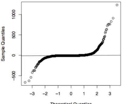
In addition, as part of our exploratory analysis we also used a regression model for investigating the relationship between the production of olives in quintal units and the surface area used for olive production. A normal probability plot of the model residuals shows a skewed distribution of the residuals and hence evidence of outlying observations (Figure 1). Given the spatial correlation in the data and the presence of outliers we decided to perform small area estimation using a small area model that employs a robust to outliers estimation method. A model of this type is the proposed spatial M-quantile model. Small area estimates of olive production per farm at LES level are therefore produced under this model using the Spatial M-quantile CD estimator. The choice of the Spatial M-quantile CD estimator is justified (i) because of the presence of outliers in the data; as Tzavidis and Chambers (2007) suggest, when outliers are present in the data the M-quantile CD estimator of the small area average is more efficient than the corresponding M-quantile estimator and (ii) because one of the targets of our analysis is to estimate the small area medians. In order to obtain consistent estimators of small area medians (and other quantiles), it is necessary to base these estimators on a consistent estimator of the small area distribution such as the Chambers-Dunstan estimator. Finally, in order to complete our comparisons we also present small area mean estimates using the EBLUP and SEBLUP estimators.
The maps in Figures 2 and 3 depict small area model estimates. Figure 2 shows the predicted values of the (a) average (Figure 2a) and (b) median (Figure 2b) of olive production per farm for each of the 42 LES areas in the Tuscany region under the Spatial M-quantile model. Figure 3 presents the small area estimates of the average of olive production per farm under EBLUP (Figure 3a) and SEBLUP (Figure 3b) estimators. We can note that EBLUP and SEBLUP estimates are very similar and they differ from the estimates obtained under the Spatial M-quantile model. The spatial distribution of M-quantile-based estimates appears to be less variable than that obtained with the traditional EBLUP and SEBLUP approaches. At this point we should also mention that in two LES areas the EBLUP and SEBLUP estimates of the small area means were negative. This can happen when there are outliers in the data that invalidate the assumptions of the linear mixed model. For these two LES areas we therefore decided to replace the negative model-based estimates (EBLUP and SEBLUP) with the corresponding direct estimates. We should also mention that we did not encounter negative small area estimates when using the M-quantile model. This is explained by the robust estimation method employed for fitting the M-quantile models.
[Figure 2 about here.] [Figure 3 about here.]
Estimates of the small area median production of olives are also obtained under the Spatial M-quantile model. The median appears to be insensitive to the presence of few big farms that raise the average level of production. The spatial distribution of the median production also appears to be more homogenous than the corresponding spatial distribution of the small area means (see Figure 2). This emphasises the importance of producing maps that represent not only the spatial distribution of the mean but also of other quantiles of the cumulative distribution function within each small area. The information contained in such maps is valuable both for agricultural policy interventions and for data users.
6. Conclusions
In this paper we propose an extension to the Chambers and Tzavidis (2006) small area M-quantile approach to allow for spatially correlated random effects. Spatial information is incorporated into the M-quantile model by modeling the M-quantile coefficients using a parametric model that allows for spatially correlated random effects. Small area estimates are then obtained by fitting an M-quantile model at the average area specific M-M-quantile coefficient predicted under this parametric model. Results from a simulation study show that this approach works well in comparison to the conventional M-quantile estimator. A drawback of our approach is that we still need to specify a fully parametric model for the unit-specific M-quantile coefficients. We are currently investigating the use of non-parametric methods to incorporate spatial information into the M-quantile approach.
Acknowledgements: The work reported here has been developed under the support of the project
PRIN Metodologie di stima e problemi non campionari nelle indagini in campo
agricolo-ambientale awarded by the Italian Government to the Universities of Florence, Cassino, Pisa and
References
Anselin, L. (1992) Spatial Econometrics: Method and Models, Kluwer Academic Publishers,
Boston.
Ballin, M., Salvi, S. (2004) Nota metodologica sul piano di campionamento adottato per l'indagine
“Struttura e produzione delle aziende agricole 2003”, Istat – Servizio Agricoltura.
Battese, G.E., Harter, R.M. and Fuller, W.A. (1988) An Error-Components Model for Prediction of
County Crop Areas Using Survey and Satellite Data. Journal of the American Statistical
Association, 83, 401, 28–36.
Bnerjee, S., Carlin, B.P. and Gelfand, A.E. (2004) Hierarchical Modeling and Analysis for Spatial
Data, Chapman & Hall, New York.
Breckling, J., Chambers, R. (1988) M-quantiles, Biometrika, 75, 4, 761-771.
Chambers, R., Dunstan, R. (1986) Estimating distribution function from survey data. Biometrika,
73, 597-604.
Chambers, R. and Tzavidis, N. (2006) M-quantile Models for Small Area Estimation, Biometrika,
93, pp. 255-268.
Chambers, R., Chandra, H. and Tzavidis, N. (2007) On robust mean squared error estimation for linear predictors for domains. [Paper submitted for publication. A copy is available upon request].
Cliff, A.D. and Ord, J.K. (1981) Spatial Processes. Models & Applications, Pion Limited, London.
Cressie, N. (1993) Statistics for spatial data, John Wiley & Sons, New York.
Datta, G.S. and Lahiri, P. (2000) A Unified Measure of Uncertainty of Estimates for Best Linear
Unbiased Predictors in Small Area Estimation Problem, Statistica Sinica, 10, 613-627.
Henderson C. (1975) Best linear unbiased estimation and prediction under a selection model,
Biometrics, 31, 423-447.
Petrucci, A. and Salvati, N. (2005) “Small Area Estimation: the Spatial EBLUP at area and at unit level”. Atti del Convegno “Metodi per l’integrazione di dati da più fonti”, Roma.
Petrucci, A., Pratesi, M. and Salvati, N. (2005) Geographic Information in Small Area Estimation:
Small Area Models and Spatially Correlated Random Area Effects, Statistics in Transition, 7, 3,
609-623.
Petrucci, A. and Salvati, N. (2006) Small Area Estimation for Spatial Correlation in Watershed
Erosion Assessment, Journal of Agricultural, Biological and Environmental Statistics, 11, 2,
169-182.
Pratesi, M. and Salvati, N. (2005) Regressione M-quantilica nella stima per piccole aree. Il caso della produzione di olive in Toscana, relazione invitata ed pubblicata negli atti del Convegno
“AGRI@STAT -Verso un nuovo sistema di statistiche agricole”, 30-31 Maggio 2005, Firenze.
Rao, J.N.K. and Choudhry, G.H. (1995) Small Area Estimation: Overview and Empirical Study in
Business Survey Method, Edited by Cox, Binder, Chinnappa, Christianson, Colledge, Kott, John
Wiley & Sons, 38, 527-540.
Rao, J.N.K. (2003) Small area estimation, John Wiley & Sons, New York.
Saei, A. and Chambers, R. (2003) Small Area Estimation Under Linear and Generalized Linear
Model With Time and Area Effects, Working Paper M03/15, Southampton Statistical Sciences
Research Institute, University of Southampton.
Salvati, N. (2004) Small Area Estimation by Spatial Models: the Spatial Empirical Best Linear
Unbiased Prediction (Spatial EBLUP), Working Paper n 2004/04, “G. Parenti” Department of
Statistics, University of Florence.
Singh, B.B., Shukla, G.K. and Kundu, D. (2005) Spatio-Temporal Models in Small Area
Estimation, Survey Methodology, 31, 2, 183-195.
Tzavidis, N. and Chambers, R. (2006) Bias adjusted estimation for small areas with outlying values.
Southampton Statistical Sciences Research Institute, Working Paper M06/09, Southampton.
Tzavidis, N. and Chambers, R. (2007) Robust prediction of small area means and distributions. Submitted for publication.
Table 1.Comparison of small area estimators !>0.
Estimator ARB(%) RRMSE(%) PRB(%)
SEBLUP 2.93 5.64 32.52 EBLUP 2.38 6.11 18.44 M-quantile 2.93 6.18 29.67 M-quantile CD 1.87 6.03 13.42 Spatial M-quantile 2.51 5.72 27.37 ! =0.75 Spatial M-quantile CD 1.55 5.81 10.96 SEBLUP 2.66 4.53 46.55 EBLUP 2.78 4.65 47.61 M-quantile 1.73 4.88 22.97 M-quantile CD 1.12 5.36 12.68 Spatial M-quantile 1.98 4.40 27.92 !=0.5 Spatial M-quantile CD 1.12 4.94 11.10 SEBLUP 2.72 4.48 47.04 EBLUP 2.69 4.39 47.81 M-quantile 1.78 4.59 21.83 M-quantile CD 1.11 4.89 10.04 Spatial M-quantile 2.12 4.39 31.06 !=0.25 Spatial M-quantile CD 1.17 4.74 11.03
Table 2. Comparison of small area estimators !<0.
Estimator ARB(%) RRMSE(%) PRB(%)
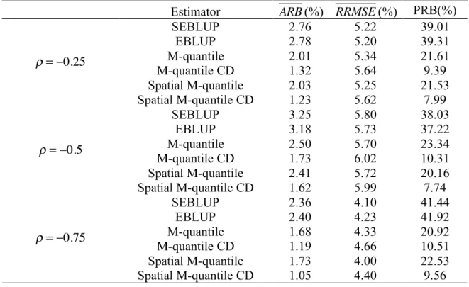
SEBLUP 2.76 5.22 39.01 EBLUP 2.78 5.20 39.31 M-quantile 2.01 5.34 21.61 M-quantile CD 1.32 5.64 9.39 Spatial M-quantile 2.03 5.25 21.53 !="0.25 Spatial M-quantile CD 1.23 5.62 7.99 SEBLUP 3.25 5.80 38.03 EBLUP 3.18 5.73 37.22 M-quantile 2.50 5.70 23.34 M-quantile CD 1.73 6.02 10.31 Spatial M-quantile 2.41 5.72 20.16 !="0.5 Spatial M-quantile CD 1.62 5.99 7.74 SEBLUP 2.36 4.10 41.44 EBLUP 2.40 4.23 41.92 M-quantile 1.68 4.33 20.92 M-quantile CD 1.19 4.66 10.51 Spatial M-quantile 1.73 4.00 22.53 !="0.75 Spatial M-quantile CD 1.05 4.40 9.56
Figure 1. Normal probability plot of the linear regression model residuals.
Figure 2. Small area estimates of the (a) average and (b) median olive production per farm in quintal units for each of the 42 LES in the Tuscany region under Spatial M-quantile model.
Figure 3. Small area estimates of the average olive production per farm in quintal units for each of the 42 LES in the Tuscany region under (a) EBLUP and (b) SEBLUP estimators.